https://doi.org/10.4224/19040608
READ THESE TERMS AND CONDITIONS CAREFULLY BEFORE USING THIS WEBSITE. https://nrc-publications.canada.ca/eng/copyright
Vous avez des questions? Nous pouvons vous aider. Pour communiquer directement avec un auteur, consultez la première page de la revue dans laquelle son article a été publié afin de trouver ses coordonnées. Si vous n’arrivez pas à les repérer, communiquez avec nous à [email protected].
Questions? Contact the NRC Publications Archive team at
[email protected]. If you wish to email the authors directly, please see the first page of the publication for their contact information.
Archives des publications du CNRC
For the publisher’s version, please access the DOI link below./ Pour consulter la version de l’éditeur, utilisez le lien DOI ci-dessous.
Access and use of this website and the material on it are subject to the Terms and Conditions set forth at
Measuring Degrees of Semantic Opposition
Mohammad, Saif M.; Dorr, Bonnie J.; Hirst, Graeme; Turney, Peter D.
https://publications-cnrc.canada.ca/fra/droits
L’accès à ce site Web et l’utilisation de son contenu sont assujettis aux conditions présentées dans le site
LISEZ CES CONDITIONS ATTENTIVEMENT AVANT D’UTILISER CE SITE WEB.
NRC Publications Record / Notice d'Archives des publications de CNRC:
https://nrc-publications.canada.ca/eng/view/object/?id=9994b07b-738c-4bcc-b884-98b4560e7566 https://publications-cnrc.canada.ca/fra/voir/objet/?id=9994b07b-738c-4bcc-b884-98b4560e7566Canada, Ottawa, Canada.
Measuring Degrees of Semantic Opposition
Saif M. Mohammad
∗National Research Council Canada
Bonnie J. Dorr
∗∗University of Maryland
Graeme Hirst
†University of Toronto
Peter D. Turney
‡National Research Council Canada
Knowing the degree of semantic contrast, or oppositeness, between words has widespread application in natural language processing, including machine translation, and information retrieval. Manually-created lexicons focus on strict opposites, such as antonyms, and have limited coverage. On the other hand, only a few automatic approaches have been proposed, and none have been comprehensively evaluated. Even though oppositeness may seem to be a simple and fairly intuitive idea at first glance, any deeper analysis quickly reveals that it is in fact a complex and heterogeneous phenomenon. In this paper we present a large crowdsourcing experiment to determine the amount of human agreement on the concept of oppositeness and its different kinds. In the process, we flesh out key features of different kinds of opposites and also determine their relative prevalence. We then present an automatic and empirical measure of lexical contrast that combines corpus statistics with the structure of a published thesaurus. Using four different datasets, we evaluated our approach on two different tasks, solving closest-to-opposite questions and distinguishing synonyms from antonyms. The results are analyzed across four parts of speech and across five different kinds of opposites. We show that our measure of lexical contrast obtains high precision and large coverage, outperforming existing methods.
Key words:lexical contrast, antonymy, kinds of opposites, distributional hypothesis, thesaurus structure, affixes, crowdsourcing, closest-to-opposite questions.
1. Introduction
Native speakers of a language intuitively recognize different degrees of lexical contrast or oppositeness—for example most people will agree that hot and cold have a higher degree of oppositeness than cold and lukewarm, and cold and lukewarm have a higher degree of oppositeness than penguin and clown. Automatically determining the degree of contrast between words has many uses, including:
∗ Institute for Information Technology, National Research Council Canada. E-mail: [email protected]
∗∗Department of Computer Science and Institute of Advanced Computer Studies, University of Maryland. E-mail: [email protected]
† Department of Computer Science, University of Toronto. E-mail: [email protected]
‡ Institute for Information Technology, National Research Council Canada. E-mail: [email protected]
r
Detecting and generating paraphrases (Marton, El Kholy, and Habash2011) (The dementors caught Sirius Black / Black could not escape the dementors).
r
Detecting certain types of contradictions (de Marneffe, Rafferty, andManning 2008; Voorhees 2008) (Kyoto has a predominantly wet climate / It is mostly dry in Kyoto). This is in turn useful in effectively re-ranking target language hypotheses in machine translation, and for re-ranking query responses in information retrieval.
r
Understanding discourse structure and improving dialogue systems.Opposites often indicate the discourse relation of contrast (Marcu and Echihabi 2002).
r
Detecting humor (Mihalcea and Strapparava 2005). Satire and jokes tendto have contradictions and oxymorons.
r
Distinguishing near-synonyms from word pairs that are semanticallycontrasting in automatically created distributional thesauri. Measures of distributional similarity typically fail to do so.
Detecting contrasting words is not sufficient by itself to solve most of these problems, but it is a crucial component.
Lexicons of pairs of words that native speakers consider strict opposites have been created for certain languages, but their coverage is limited. They mostly only include pairs of opposing gradable adjectives called antonyms. Further, contrasting word pairs far outnumber those that are commonly considered strict opposites. In our own ex-periments described later in this paper, we find that more than 90% of the contrasting pairs in GRE closest-to-opposite questions are not listed as opposites in WordNet. Even though a number of computational approaches have been proposed for semantic close-ness (Budanitsky and Hirst 2006; Curran 2004), and some for hypernymy–hyponymy (Hearst 1992), measures of lexical contrast have been less successful. To some extent, this is because lexical contrast is not as well understood as other classical lexical-semantic relations.
Over the years, many definitions of opposites have been proposed by linguists (Cruse 1986; Lehrer and Lehrer 1982), cognitive scientists (Kagan 1984), psycholinguists (Deese 1965), and lexicographers (Egan 1984), which differ from each other in small and large respects. One reason for this is that opposites are not a homogeneous class—there are many kinds of opposites such as antipodals, complementaries, and reversives (de-scribed in more detail in Section 3). However, there is no large-scale study determining the amount of human agreement and prevalence of different kinds of opposites. None of the proposed automatic measures of lexical contrast have so far been systematically evaluated to determine how well they capture different kinds of opposites.
In Mohammad et al. (2008) we proposed a measure of lexical contrast that combines corpus statistics with the structure of a published thesaurus. The measure was evalu-ated on about 1100 closest-to-opposite questions used as preparation for the Graduate Record Examination (GRE). This paper goes beyond Mohammad et al. (2008), and makes the following contributions:
r
We present a questionnaire designed to acquire annotations aboutcontrasting word pairs. Since the annotations were done through
of the annotators, we devoted extra effort in making sure that the questions were phrased in a simple, yet clear manner.
r
We present a quality control method that uses a word-choice question toautomatically identify and discard erroneous annotations.
r
We publicly release a new dataset of five different kinds of opposites.r
We determine the amount of agreement among humans in identifyinglexical contrast, and also in identifying different kinds of contrast.
r
We determine the prevalence of difference kinds of opposites and showthat a large number of opposing word pairs have properties pertaining to more than one kind of opposite.
r
We show that opposites co-occur significantly more often thansynonymous words. We also show that the average distributional similarity of opposites is higher than that of synonymous words.
r
We describe how we automatically generated a new set of 1296closest-to-opposite questions to evaluate performance of our method on five different kinds of opposites and across four parts of speech.
r
We evaluate the measures of contrast on the task of separating oppositesfrom synonyms using the datasets described by Lin et al. (2003) and Turney (2008), and compare performance of our method with theirs. We show that the proposed measure of lexical contrast obtains high precision and large coverage, outperforming existing methods.
We begin with a summary of related work in Section 2. In Section 3, we discuss different kinds of opposites or contrasts. In Section 4, we describe a crowdsourced survey to determine the amount of agreement among humans in identifying lexical contrast and the kinds of lexical contrast. The survey provides a wealth of additional information too, such as the prevalence of different kinds of opposites and how often a word pair may correspond to more than one kind of opposite. We present experiments that examine the manifestation of opposites in text (Section 5). We then propose an empirical approach to determining the degree of contrast between two words (Sec-tion 6). Sec(Sec-tion 7 describes experiments in which we use four different datasets to evaluate our approach on two different tasks, solving closest-to-opposite questions and distinguishing synonyms from antonyms. We demonstrate that the method yields high precision and large coverage, outperforming existing methods. Section 8 recapitulates our findings and outlines future work. All of the data created and compiled as part of this research is summarized in Table 18 (Section 8), and is available for download.1
2. Related work
Charles and Miller (1989) proposed that opposites occur together in a sentence more often than chance. This is known as the co-occurrence hypothesis. Justeson and Katz (1991) gave evidence in support of the hypothesis using 35 prototypical opposites (from an original set of 39 opposites compiled by Deese (1965)) and also with an additional 22 frequent opposites. They also showed that opposites tend to occur in parallel syntactic constructions. All of these pairs were adjectives. Fellbaum (1995) conducted similar experiments on 47 noun, verb, adjective, and adverb pairs (noun–noun, noun–verb, noun–adjective, verb–adverb and so on) pertaining to 18 concepts (for example, lose(v)–
gain(n) and loss(n)–gain(n), where lose(v) and loss(n) pertain to the concept of “failing to have/maintain”). However, non-opposite semantically related words also tend to occur together more often than chance. Thus, separating opposites from these other classes has proven to be difficult.
Some automatic methods of lexical contrast rely on lexical patterns in text, for exam-ple, Lin et al. (2003) used patterns such as “from X to Y ” and “either X or Y ” to separate opposites from distributionally similar pairs. They evaluated their method on 80 pairs of opposites and 80 pairs of synonyms taken from the Webster’s Collegiate Thesaurus (Kay 1988). The evaluation set of 160 word pairs was chosen such that it included only high-frequency terms. This was necessary to increase the probability of finding sentences in a corpus where the target pair occurred in one of the chosen patterns. Lobanova et al. (2010) used a set of Dutch adjective seed pairs to learn lexical patterns commonly containing opposites. The patterns were in turn used to create a larger list of Dutch opposites. The method was evaluated by comparing entries to Dutch lexical resources and by asking human judges to determine whether an automatically found pair is indeed an opposite. Turney (2008) proposed a supervised method for identifying synonyms, opposites, hypernyms, and other lexical-semantic relations between word pairs. The approach learns patterns corresponding to different relations.
Harabagiu et al. (2006) detected opposites for the purpose of identifying contradic-tions by using WordNet chains—synsets connected by the hypernymy–hyponymy links and exactly one antonymy link. Lucerto et al. (2002) proposed detecting opposites using the number of tokens between two words in text and also cue words such as but, from, and and. Unfortunately, they evaluated their method on only 18 word pairs. Neither Harabagiu et al. nor Lucerto et al. determined the degree of contrast between words and their methods have not been shown to have substantial coverage.
Schwab et al. (2002) created an oppositeness vector for a target word. The closer this vector is to the context vector of the other target word, the more opposite the two target words are. However, the oppositeness vectors were manually created. Further, the approach was not evaluated on more than a handful of word pairs.
There is a large amount of work on sentiment analysis and opinion mining aimed at determining the polarity of words (Pang and Lee 2008). For example, Pang, Lee, and Vaithyanathan (2002) detected that adjectives such as dazzling, brilliant, and gripping cast their qualifying nouns positively whereas adjectives such as bad, cliched, and boring portray the noun negatively. Many of these gradable adjectives have opposites, but these approaches, with the exception of Hatzivassiloglou and McKeown (1997), did not attempt to determine pairs of positive and negative polarity words that are opposites. Hatzivassiloglou and McKeown (1997) proposed a supervised algorithm that uses word usage patterns to generate a graph with adjectives as nodes. An edge between two nodes indicates either that the two adjectives have the same or opposite polarity. A clustering algorithm then partitions the graph into two subgraphs such that the nodes in a subgraph have the same polarity. They used this method to create a lexicon of positive and negative words, and argued that the method could also be used to detect opposites.
Since opposites are similar to each other in many respects, but very dissimilar in one respect, it is possible to use semantic similarity algorithms, such as the ones proposed by Turney (2001) and Gaume et al. (2006), as part of the process of identifying lexical contrast. Our approach uses pointwise mutual information (PMI), a commonly used technique to identify semantic similarity (Church and Hanks 1990; Turney 2001). However, an additional signal of contrast must be detected, and this is non-trivial because opposites, unlike synonyms, can be of many different kinds.
3. The Heterogeneous Nature of Opposites
Many different classifications of opposites have been proposed, one of which can be found in Cruse (1986) (Chapters 9, 10, and 11). It consists of complementaries (open– shut, dead–alive), antonyms (long–short, slow–fast) (further classified into polar, overlap-ping, and equipollent opposites), directional opposites (up–down, north–south) (further classified into antipodals, counterparts, and reversives), relational opposites (husband– wife, predator–prey), indirect converses (give–receive, buy–pay), congruence variants (huge– little, doctor–patient), and pseudo opposites (black–white).
Various lexical relations have also received attention at the Educational Testing Services (ETS), as analogies and closest-to-opposite questions are part of the tests they conduct. They classify opposites into contradictories (alive–dead, masculine–feminine), contraries (old–young, happy-sad), reverses (attack–defend, buy–sell), directionals (front– back, left–right), incompatibles (happy–morbid, frank–hypocritical), asymmetric contraries (hot–cool, dry–moist), pseudoopposites (popular–shy, right–bad), and defectives (default– payment, limp–walk) (Bejar, Chaffin, and Embretson 1991).
Keeping in mind the meanings and subtle distinctions between each of these kinds of opposites is not easy even if we provide extensive training to annotators. Since we crowdsource the annotations, and we know that Turkers prefer to spend their time do-ing the task (and makdo-ing money) rather than readdo-ing lengthy descriptions, we focused only on five kinds of opposites that we believed would be easiest to annotate, and which still captured a majority of the opposites:
r
Antipodals(top–bottom, start–finish): Antipodals are opposites in which“one term represents an extreme in one direction along some salient axis, while the other term denotes the corresponding extreme in the other direction” (Cruse 1986).
r
Complementaries(open–shut, dead–alive): The essential characteristic of apair of complementaries is that “between them they exhaustively divide the conceptual domain into two mutually exclusive compartments, so that what does not fall into one of the compartments must necessarily fall into the other” (Cruse 1986).
r
Disjoint(hot–cold, like–dislike): Disjoint opposites are word pairs thatoccupy non-overlapping regions in the semantic dimension such that there are regions not covered by either term. This set of opposites includes equipollent adjective pairs (for example, hot–cold) and stative verb pairs (for example, like–dislike). We refer the reader to Sections 9.4 and 9.7 of Cruse (1986) for details about these sub-kinds of opposites.
r
Gradable opposites(long–short, slow–fast): are adjective-pair oradverb-pair opposites that are gradable, that is, “members of the pair denote degrees of some variable property such as length, speed, weight, accuracy, etc” (Cruse 1986).
r
Reversibles(rise–fall, enter–exit): Reversibles are opposite verb pairs suchthat “if one member denotes a change from A to B, its reversive partner denotes a change from B to A” (Cruse 1986).
4. Crowdsourcing
In order to obtain annotations, we used Amazon’s Mechanical Turk (AMT) service. We broke the task into small independently solvable units called HITs (Human Intelligence
Table 1
Target word pairs chosen for annotation. Each term was annotated about 8 times. part of speech # of word pairs
adverbs 185
adjectives 646
nouns 416
verbs 309
all 1556
Tasks) and uploaded them on the AMT website.2Each HIT had a set of questions, all of which were to be answered by the same person (a Turker, in AMT parlance). We created HITs for word pairs, taken from WordNet, that we expected to have some degree of contrast in meaning.
In WordNet, words that are close in meaning are grouped together in a set called a synset. If one of the words in a synset is a direct opposite of another word in a different synset, then the two synsets are called head synsets (Gross, Fischer, and Miller 1989). Other word pairs across the two head synsets form indirect opposites. We chose as target pairs all direct and indirect opposites from WordNet that were also listed in the Macquarie Thesaurus. This condition was a mechanism to ignore less-frequent and obscure words, and apply our resources on words that are more common. Additionally, as we will describe ahead, we use the presence of the words in the thesaurus to help generate Question 1, which we use for quality control of the annotations. Table 1 gives a breakdown of the 1,556 pairs chosen by part of speech.
Since we do not have any control over the educational background of the anno-tators, we made efforts to phrase questions about the kinds of opposites in a simple and clear manner. Therefore we avoided definitions and long instructions in favor of examples and short questions. We believe this strategy is beneficial even in traditional annotation scenarios.
We created separate questionnaires (HITs) for adjectives, adverbs, nouns, and verbs. A complete example adjective HIT with directions and questions is shown in Figure 1. The adverb, noun, and verb questionnaires had similar questions, but were phrased slightly differently to accommodate differences in part of speech. These questionnaires are not shown here due lack of space, but all four questionnaires are available for download.3The verb questionnaire had an additional question shown in Figure 2. Since nouns and verbs are not considered gradable, the corresponding questionnaires did not have Q8 and Q9. We requested annotations from eight different Turkers for each HIT.
4.1 The Word Choice Question: Q1
Q1 is an automatically generated word choice question that has a clear correct answer. It helps identify erroneous and malicious annotations. If this question is answered incorrectly, then we assume that the annotator does not know the meanings of the target words, and we ignore responses to the remaining questions. Further, as this question makes the annotator think about the meanings of the words and about the relationship between them, we believe it improves the responses for subsequent questions.
2 https://www.mturk.com/mturk/welcome
Word-pair: musical×dissonant
Q1.Which set of words is most related to the word pair musical:dissonant?
r
useless, surgery, ineffectual, institution
r
sequence, episode, opus, composition
r
youngest, young, youthful, immature
r
consequential, important, importance, heavyQ2.Do musical and dissonant have some contrast in meaning?
r
yesr
noFor example, up–down, lukewarm–cold, teacher–student, attack–defend, all have at least some degree of contrast in meaning. On the other hand, clown–down, chilly–cold, teacher–doctor, and attack–rush DO NOT have contrasting meanings.
Q3.Some contrasting words are paired together so often that given one we naturally think of the other. If one of the words in such a pair were replaced with another word of almost the same meaning, it would sound odd. Are musical:dissonant such a pair?
r
yesr
noExamples for “yes”: tall–short, attack–defend, honest–dishonest, happy–sad. Examples for “no”: tall–stocky, attack–protect, honest–liar, happy–morbid.
Q5.Do musical and dissonant represent two ends or extremes?
r
yesr
noExamples for “yes”: top–bottom, basement–attic, always–never, all–none, start–finish. Examples for “no”: hot–cold (boiling refers to more warmth than hot and freezing refers to less warmth than cold), teacher–student (there is no such thing as more or less teacher and more or less student), always–sometimes (never is fewer times than sometimes).
Q6.If something is musical, would you assume it is not dissonant, and vice versa? In other words, would it be unusual for something to be both musical and dissonant?
r
yesr
noExamples for “yes”: happy–sad, happy–morbid, vigilant–careless, slow–stationary. Examples for “no”: happy–calm, stationary–still, vigilant–careful, honest–truthful.
Q7.If something or someone could possibly be either musical or dissonant, is it necessary that it must be either musical or dissonant? In other words, is it true that for things that can be musical or dissonant, there is no third possible state, except perhaps under highly unusual circumstances?
r
yesr
noExamples for “yes”: partial–impartial, true–false, mortal–immortal.
Examples for “no”: hot–cold (an object can be at room temperature is neither hot nor cold), tall–short (a person can be of medium or average height).
Q8.In a typical situation, if two things or two people are musical, then can one be more musical than the other?
r
yesr
noExamples for “yes”: quick, exhausting, loving, costly. Examples for “no”: dead, pregnant, unique, existent.
Q9.In a typical situation, if two things or two people are dissonant, can one be more dissonant than the other?
r
yesr
noExamples for “yes”: quick, exhausting, loving, costly, beautiful. Examples for “no”: dead, pregnant, unique, existent, perfect, absolute.
Figure 1
Example HIT: Adjective pairs questionnaire.
Note: Perhaps “musical×dissonant” might be better written as “musical versus dissonant”, but we have kept “×” here to show the reader exactly what the Turkers were given.
Note: Q4 is not shown here, but can be seen in the online version of the questionnaire. It was an exploratory question, and it was not multiple choice. Q4’s responses have not been analyzed.
Word-pair: enabling×disabling
Q10.In a typical situation, do the sequence of actions disabling and then enabling bring someone or something back to the original state, AND do the sequence of actions enabling and disabling also bring someone or something back to the original state?
r
yes, both ways: the transition back to the initial state makes much sense in both sequences.r
yes, but only one way: the transition back to the original state makes much more sense oneway, than the other way.
r
none of the aboveExamples for “yes, both ways”: enter–exit, dress–undress, tie–untie, appear–disappear. Examples for “yes, but only one way”: live–die, create–destroy, damage–repair, kill–resurrect. Examples for “none of the above”: leave–exit, teach–learn, attack–defend (attacking and then defending does not bring one back to the original state).
Figure 2
Additional question in the questionnaire for verbs.
Table 2
Number of word pairs and average number of annotations per word pair in the master set. part of # of average # of
speech word pairs annotations
adverbs 182 7.80
adjectives 631 8.32
nouns 405 8.44
verbs 288 7.58
all 1506 8.04
The options for Q1 were generated automatically. Each option is a set of four comma-separated words. The words in the answer are close in meaning to both of the target words. In order to create the answer option, we first generated a much larger source pool of all the words that were in the same thesaurus category as any of the two target words. (Words in the same category are closely related.) Words that had the same stem as either of the target words were discarded. For each of the remaining words, we added their Lesk similarities with the two target words (Banerjee and Pedersen 2003). The four words with the highest sum were chosen to form the answer option.
The three distractor options were randomly selected from the pool of correct answers for all other word choice questions. Finally, the answer and distractor options were presented to the Turkers in random order.
4.2 Post-Processing
The response to a HIT by a Turker is called an assignment. We obtained about 12,448 assignments in all (1556 pairs×8 assignments each). About 7% of the adjective, verb, and noun assignments and about 13% of the verb assignments had an incorrect answer to Q1. These assignments were discarded, leaving 1506 target pairs with three or more valid assignments. We will refer to this set of assignments as the master set, and all further analysis in this paper is based on this set. Table 2 gives a breakdown of the average number of annotations for each of the target pairs in the master set.
Table 3
Percentage of word pairs that received a response of “yes” for the questions in the questionnaire. ‘adj.’ stands for adjectives. ‘adv.’ stands for adverbs.
% of word pairs
Question answer adj. adv. nouns verbs
Q2. Do X and Y have some contrast? yes 99.5 96.8 97.6 99.3
Q3. Are X and Y opposites? yes 91.2 68.6 65.8 88.8
Q5. Are X and Y at two ends of a dimension? yes 81.8 73.5 81.1 94.4
Q6. Does X imply not Y? yes 98.3 92.3 89.4 97.5
Q7. Are X and Y mutually exhaustive? yes 85.1 69.7 74.1 89.5 Q8. Does X represent a point on some scale? yes 78.5 77.3 - -Q9. Does Y represent a point on some scale? yes 78.5 70.8 -
-Q10. Does X undo Y OR does Y undo X? one way - - - 3.8
both ways - - - 90.9
Table 4
Percentage of WordNet source pairs that are contrasting, opposite, and “contrasting but not opposite”.
category basis adj. adv. nouns verbs
contrasting Q2 yes 99.5 96.8 97.6 99.3
opposites Q2 yes and Q3 yes 91.2 68.6 60.2 88.9
contrasting, but not opposite Q2 yes and Q3 no 8.2 28.2 37.0 10.4
4.3 Prevalence of Different Kinds of Contrasting Pairs
For each question pertaining to every word pair in the master set, we determined the most frequent response by the annotators. Table 3 gives the percentage of word-pairs in the master set that received a most frequent response of “yes”. The first column in the table lists the question number followed by a brief description of question. (Note that the Turkers saw only the full forms of the questions, as shown in the example HIT.)
Observe that most of the word pairs are considered to have at least some contrast in meaning. This is not surprising since the master set was constructed using words connected through WordNet’s antonymy relation. Responses to Q3 show that not all contrasting pairs are considered opposite, and this is especially the case for adverb pairs and noun pairs. The rows in Table 4 show the percentage of words in the master set that are contrasting (row 1), opposite (row 2), and contrasting but not opposite (row 3).
Responses to Q5, Q6, Q7, Q8, and Q9 (Table 3) show the prevalence of different kinds of relations and properties of the target pairs.
Table 5 shows the percentage of contrasting word pairs that may be classified into the different types discussed in Section 3 earlier. Observe that rows for all categories other than the disjoints have percentages greater than 60%. This means that a number of contrasting word pairs can be classified into more than one kind. Complementaries are the most common kind in case of adverbs, nouns, and verbs, whereas antipodals are most common among adjectives. A majority of the adjective and adverb contrasting pairs are gradable, but more than 30% of the pairs are not. Most of the verb pairs are reversives (91.6%). Disjoint pairs are much less common than all the other categories considered, and they are most prominent among adjectives (28%), and least among verb pairs (1.7%).
Table 5
Percentage of contrasting word pairs belonging to various sub-types. The sub-type “reversives" applies only to verbs. The sub-type “gradable" applies only to adjectives and adverbs.
sub-type basis adv. adj. nouns verbs
Antipodals Q2 yes, Q5 yes 82.3 75.9 82.5 95.1
Complementaries Q2 yes, Q7 yes 85.6 72.0 84.8 98.3
Disjoint Q2 yes, Q7 no 14.4 28.0 15.2 1.7
Gradable Q2 yes, Q8 yes, Q9 yes 69.6 66.4 -
-Reversives Q2 yes, Q10 both ways - - - 91.6
Table 6
Breakdown of answer agreement by target-pair part of speech and question: For every target pair, a question is answered by about eight annotators. The majority response is chosen as the answer. The ratio of the size of the majority and the number of annotators is indicative of the amount of agreement. The table below shows the average percentage of this ratio.
question adj. adv. nouns verbs average
Q2. Do X and Y have some contrast? 90.7 92.1 92.0 94.7 92.4
Q3. Are X and Y opposites? 79.0 80.9 76.4 75.2 77.9
Q5. Are X and Y at two ends of a dimension? 70.3 66.5 73.0 78.6 72.1
Q6. Does X imply not Y? 89.0 90.2 81.8 88.4 87.4
Q7. Are X and Y mutually exhaustive? 70.4 69.2 78.2 88.3 76.5 average (Q2, Q3, Q5, Q6, and Q7) 82.3 79.8 80.3 85.0 81.3
Q8. Does X represent a point on some scale? 77.9 71.5 - - 74.7
Q9. Does Y represent a point on some scale? 75.2 72.0 - - 73.6
Q10. Does X undo Y OR does Y undo X? - - - 73.0 73.0
4.4 Agreement
People do not always agree on linguistic classifications of terms, and one of the goals of this work was to determine how much people agree on properties relevant to different kinds of opposites. Table 6 lists the breakdown of agreement by target-pair part of speech and question, where agreement is the average percentage of the number of Turkers giving the most-frequent response to a question—the higher the number of Turkers that vote for the majority answer, the higher is the agreement.
Observe that agreement is highest when asked whether a word pair has some degree of contrast in meaning or not (Q2), and that there is a marked drop when asked if the two words are opposites (Q3). This is true for each of the parts of speech, although the drop is highest for verbs (94.7% to 75.2%).
For questions 5 through 9, we see varying degrees of agreement—Q6 obtaining the highest agreement and Q5 the lowest. We observe marked difference across parts of speech for certain questions. For example, verbs are the easiest part of speech to identify (highest agreement for Q5, Q7, and Q8). For Q6, nouns have markedly lower agreement than all other parts of speech—not surprising considering that the set of disjoint opposites is traditionally associated with equipollent adjectives and stative verbs. Adverbs and adjectives have markedly lower agreement scores for Q7 than nouns and verbs.
5. Clues for contrast from occurrences in text
Here we investigate the tendency of opposites to co-occur in text (Section 5.1), and their tendency to occur in similar contexts (Section 5.2).
As pointed out earlier, there is work on a small set of opposites showing that opposites co-occur more often than chance (Charles and Miller 1989; Fellbaum 1995). Section 5.1 describes experiments on a larger scale to determine whether opposites in-deed occur together more often than randomly chosen word pairs of similar frequency. The section also compares co-occurrence associations of opposites and synonyms to determine whether they are similar or different.
Research in distributional similarity has found that entries in distributional thesauri tend to also contain terms that are opposite in meaning (Lin 1998; Lin et al. 2003). Section 5.2 describes experiments to determine whether opposite words occur in similar contexts as often as randomly chosen pairs of words with similar frequencies, and whether opposite words occur in similar contexts as often as synonyms.
5.1 The co-occurrence hypothesis of opposites
In order to compare the tendencies of opposites, synonyms, and random word pairs to co-occur in text, we created three sets of word pairs: the opposites set, the synonyms set, and the control set of random word pairs, First we selected all the opposites (nouns, verbs, and adjectives) from WordNet. We discarded pairs that did not meet the following conditions: (1) both members of the pair must be unigrams, (2) both members of the pair must occur in the British National Corpus (BNC) (Burnard 2000), and (3) at least one member of the pair must have a synonym in WordNet. A total of 1358 word pairs remained, and these form the opposites set.
Each of the pairs in the opposites set was used to create a synonym pair by choosing a WordNet synonym of exactly one member of the pair.4If a word has more than one synonym, then the most frequent synonym is chosen.5These 1358 word pairs form the synonyms set. Note that for each of the pairs in the opposites set, there is a correspond-ing pair in the synonyms set, such that the two pairs have a common term. For example, the pair agitation and calmness in the opposites set, has a corresponding pair agitation and ferment in the synonyms set. We will refer to the common terms (agitation in the above example) as the focus words. Since we also wanted to compare occurrence statistics of the opposites set with the random pairs set, we created the control set of random pairs by taking each of the focus words and pairing them with another word in WordNet that has a frequency of occurrence in BNC closest to the opposite of the focus word. This is to ensure that members of the pairs across the opposites set and the control set have similar unigram frequencies.
We calculated the pointwise mutual information (PMI) (Church and Hanks 1990) for each of the word pairs in the opposites set, the random pairs set, and the synonyms set using unigram and co-occurrence frequencies in the BNC. If two words occurred within a window of five adjacent words in a sentence, they were marked as co-occurring (same window as what Church and Hanks (1990) used in their seminal work on word– word associations). Table 7 shows the average and standard deviation in each set.
4 If both members of a pair have WordNet synonyms, then one is randomly chosen at random, and its synonym is taken.
Table 7
Pointwise mutual information (PMI) of word pairs. High positive values imply a tendency to co-occur in text more often than random chance.
average PMI standard deviation
opposites set 1.471 2.255
random pairs set 0.032 0.236
synonyms set 0.412 1.110
Table 8
Distributional similarity of word pairs. The measure proposed in Lin (1998) was used. average distributional similarity standard deviation
opposites set 0.064 0.071
random pairs set 0.036 0.034
synonyms set 0.056 0.057
Observe that opposites have a much higher tendency to co-occur than the random pairs control set, and also the synonyms set. However, the opposites set has a large standard deviation. A two-sample t-test revealed that the opposites set is significantly different from the random set (p<0.05), and also that the opposites set is significantly different
from the synonyms set (p<0.05).
However, on average the PMI between a focus word and its opposite was lower than the PMI between the focus word and 3559 other words in the BNC. These were often words related to the focus words, but nether opposite nor synonymous. Thus, even though a high tendency to co-occur is a feature of opposites, it is not a sufficient condition for detecting opposites. We use PMI as part of our method for determining the degree of lexical contrast (described ahead in Section 6).
5.2 The substitutional and distributional hypotheses of opposites
Charles and Miller (1989) proposed that in most contexts, opposite may be inter-changed. The meaning of the utterance will be inverted, of course, but the sentence will remain grammatical and linguistically plausible. This came to be known as the substitutability hypothesis. However, their experiments did not support this claim. They found that given a sentence with the target adjective removed, most people did not confound the missing word with its opposite. Justeson and Katz (1991) later showed that in sentences that contain both members of an adjectival opposite pair, the target adjectives do indeed occur in similar syntactic structures at the phrasal level. From this, we can formulate the distributional hypothesis of opposites: opposites occur in similar contexts more often than non-contrasting word pairs.
We used the same sets of opposites, synonyms, and random pairs described in the previous sub-section to gather empirical proof of the distributional hypothesis. We calculated the distributional similarity between each pair in the three sets using Lin’s (1998) measure. Table 8 shows the average and standard deviation in each set. Observe that opposites have a much higher average distributional similarity than the random pairs control set, and interestingly it is also higher than the synonyms set. Once again, the opposites set has a large standard deviation. A two-sample t-test revealed that the opposites set is significantly different from both the random set and the synonyms set
with a confidence interval of 0.05. This demonstrates that relative to other word pairs, opposites tend to occur in similar contexts. We also find that the synonyms set has a significantly higher distributional similarity than the random pairs set (p<0.05). This
shows that near-synonymous word pairs also occur in similar contexts (the distribu-tional hypothesis of similarity). Further, a consequence of the large standard deviations in the cases of both opposites and synonyms means that distributional similarity alone is not sufficient to determine whether two words are opposites or synonyms. An auto-matic method for recognizing contrast will require additional cues. Our method uses PMI and other sources of information described in the next section. It does not use distributional similarity.
6. Determining Lexical Contrast
In this section, we recapitulate the automatic method for determining lexical contrast that we first proposed in Mohammad et al. (2008). Additional details are provided regarding the lexical resources used (Section 6.1) and the method itself (Section 6.2).
6.1 Lexical Resources
Our method makes use of a published thesaurus and co-occurrence information from text. Optionally, it can use opposites listed in WordNet if available. We briefly describe these resources here.
6.1.1 Published thesauri.Published thesauri, such as Roget’s and Macquarie, divide the vocabulary of a language into about a thousand categories. Words within a category tend to pertain to a coarse concept. Each category is represented by a category number (unique ID) and a head word — a word that best represents the meanings of the words in the category. One may also find opposites in the same category, but this is rare. Words with more than one meaning may be found in more than one category; these represent its coarse senses.
Within a category, the words are grouped into finer units called paragraphs. Words in the same paragraph are closer in meaning than those in differing paragraphs. Each paragraph has a paragraph head — a word that best represents the meaning of the words in the paragraph. Words in a thesaurus paragraph belong to the same part of speech. A thesaurus category may have multiple paragraphs belonging to the same part of speech. For example, a category may have three noun paragraphs, four verb paragraphs, and one adjective paragraph. We will take advantage of the structure of the thesaurus in our approach.
6.1.2 WordNet.As mentioned earlier, WordNet encodes certain strict opposites. How-ever, we found in our experiments (Section 7 below) that more than 90% of near-opposites included in Graduate Record Examination (GRE) closest-to-opposite ques-tions are not encoded in WordNet.6 Also, neither WordNet nor any other manually-created repository of opposites provides the degree of contrast between word pairs. Nevertheless, we investigate the usefulness of WordNet as a source of seed opposites for our approach.
6 GRE is a graduate admissions test taken by hundreds of thousands of prospective graduate and business school applicants. The test is administered by Educational Testing Service (ETS).
Table 9
Fifteen affix patterns used to generate opposites. Here ‘X’ stands for any sequence of letters common to both words w1and w2.
affix pattern
pattern # word 1 word 2 # word pairs example pair
1 X antiX 41 clockwise–anticlockwise 2 X disX 379 interest–disinterest 3 X imX 193 possible–impossible 4 X inX 690 consistent–inconsistent 5 X malX 25 adroit–maladroit 6 X misX 142 fortune–misfortune 7 X nonX 72 aligned–nonaligned 8 X unX 833 biased–unbiased 9 lX illX 25 legal–illegal 10 rX irrX 48 regular–irregular
11 imX exX 35 implicit–explicit
12 inX exX 74 introvert–extrovert
13 upX downX 22 uphill–downhill
14 overX underX 52 overdone–underdone
15 Xless Xful 51 harmless–harmful
Total: 2682
6.2 Proposed Measure of Lexical Contrast
We now present an empirical approach to determining lexical contrast. The approach has two parts: (1) determining whether the target word pair is contrasting or not, and (2) determining the degree of contrast between the words.
6.2.1 Detecting whether the target pair is contrasting. We first determine pairs of thesaurus categories that are contrasting in meaning using the three methods described below. Any of these methods may be used alone or in combination with others. If the target words belong to two contrasting categories, then they are assumed to be contrasting as well.
Method using affix-generated seed set. Strict opposites such as hot–cold and dark–light occur frequently in text, but in terms of type-pairs they are outnumbered by those created using affixes, such as un- (clear–unclear) and dis- (honest–dishonest). Further, this phenomenon is observed in most languages (Lyons 1977).
Table 9 lists fifteen affix patterns that tend to generate opposites in English. They were compiled by the first author by examining a small list of affixes for the English language.7These patterns were applied to all words in the thesaurus that are at least three characters long. If the resulting term was also a valid word in the thesaurus, then the word-pair was added to the affix-generated seed set. These fifteen rules generated 2,682 word pairs when applied to the words in the Macquarie Thesaurus. Category pairs that had these opposites were marked as contrasting. Of course, not all of the word pairs generated through affixes are truly opposites, for example sect–insect and part–impart. For now, such pairs are sources of error in the system. Manual analysis of these 2,682
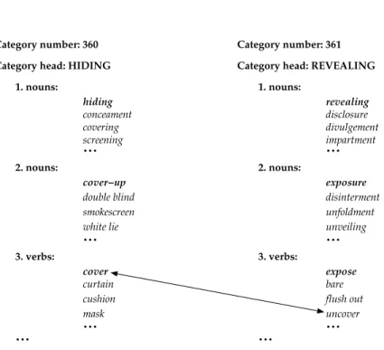
3. verbs: hiding conceament covering screening
...
cover−up double blind smokescreen white lie...
cover mask...
curtain cushion 3. verbs: 1. nouns: Category number: 360 Category head: HIDING2. nouns:
...
Category number: 361 Category head: REVEALING
1. nouns:
...
...
divulgement disclosure...
uncover flush out...
disinterment revealing exposure expose impartment unfoldment unveiling bare 2. nouns: Figure 3Example contrasting category pair. The system identifies the pair to be contrasting through the affix-based seed pair cover–uncover. The paragraphs of cover and expose are referred to as prime contrasting paragraphs. Paragraph heads are shown in bold italic.
word pairs can help determine whether this error is large or small. (We have released the full set of word pairs.) However, evaluation results (Section 7) indicate that these seed pairs improve the overall accuracy of the system.
Figure 3 presents such an example pair. Observe that categories 360 and 361 have the words cover and uncover, respectively. Affix pattern 8 from Table 1 produces seed pair cover–uncover, and so the system concludes that the two categories have contrasting meaning. The contrast in meaning is especially strong for the paragraphs cover and expose because words within these paragraphs are very close in meaning to cover and uncover, respectively. We will refer to such thesaurus paragraph pairs that have one word each of a seed pair as prime contrasting paragraphs. We expect the words across prime contrasting paragraphs to have a high degree of antonymy (for example, mask and bare), whereas words across other contrasting category paragraphs may have a smaller degree of antonymy as the meaning of these words may diverge significantly from the meanings of the words in the prime contrasting paragraphs (for example, white lie and disclosure).
Method using WordNet seed set. We compiled a list of 20,611 semantically contrasting pairs from WordNet. If two words from two synsets in WordNet are connected by an antonymy link, then every term across the two synsets was considered to be semanti-cally contrasting. A large number of them include multiword expressions. Only 10,807 of the 20,611 pairs have both words in the Macquarie Thesaurus—the vocabulary used for our experiments. We will refer to them as the WordNet seed set. Category pairs that had these opposites were marked as contrasting.
Method using adjacency of thesaurus categories. Most published thesauri, such as Roget’s, are organized such that contrasting categories are placed next to each other. For exam-ple, in the Macquarie Thesaurus: category 369 is about honesty and category 370 is about dishonesty; as shown in Figure 3, category 360 is about hiding and category 361 is about revealing. There are a number of exceptions to this rule, and often a category may be contrasting in meaning to several other categories. However, since this was an easy-enough heuristic to implement, we investigated the usefulness of considering adjacent thesaurus categories as contrasting. We will refer to this as the adjacency heuristic.
To determine how accurate the adjacency heuristic is, the first author manually inspected adjacent thesaurus categories in the Macquarie Thesaurus to determine which of them were indeed contrasting. Since a category, on average, has about a hundred words, the task was made less arduous by representing each category by just the first ten words listed in it. This way it took only about five hours to manually determine that 209 pairs of the 811 adjacent Macquarie category pairs were contrasting. Twice, it was found that category number X was contrasting not just to category number X+1 but also to category number X+2: category 40 (ARISTOCRACY) has a meaning that contrasts that of category 41 (MIDDLE CLASS) as well as category 42 (WORKING CLASS); category 542 (PAST) contrasts with category 543 (PRESENT) as well as category 544 (FUTURE). Both these X–(X+2) pairs are also added to the list of manually annotated contrasting categories.
6.2.2 Computing the degree of contrast.Relying on the co-occurrence hypothesis, we claim that the degree of contrast between two words listed in two contrasting categories is directly proportional to their tendency to co-occur in text. We use PMI to capture the tendency of word–word co-occurrence. We collected these co-occurrence statistics from the Google n-gram corpus (Brants and Franz 2006), which was created from a text collection of over 1 trillion words. Words that occurred within a window of 5 words were considered to be co-occurring.
We expected that some features may be more accurate than others. If multiple features give evidence towards opposing information, then it is useful for the system to know which feature is more reliable. Therefore, we held out some data from the evaluation data described in Section 7.1 as the development set. Experiments on the development set showed that contrasting words may be placed in three bins corre-sponding to the amount of reliability of the source feature: high, medium, or acceptable.
r
high reliability (Class I):target words that belong to adjacent thesauruscategories. For example, all the word pairs across categories 360 and 361, shown in Figure 3. Examples of class I contrasting word pairs from the development set include graceful–ungainly, fortunate–hapless, obese–slim, and effeminate–virile. (Note, there need not be any affix or WordNet seed pairs across adjacent thesaurus categories for these word pairs to be marked Class I.)
r
medium reliability (Class II):target words that are not Class I opposites,but belong to one paragraph each of a prime contrasting paragraph. For example, all the word pairs across the paragraphs of sympathetic and indifferent. See Figure 4. Examples of class II contrasting word pairs from the development set include altruism–avarice, miserly–munificent,
accept–repudiate, and improper–prim.
r
acceptable reliability (Class III):target words that are not Class I or Class1. nouns: Category number: 423 Category head: KINDNESS
1. nouns: Category number: 230 Category head: APATHY
kindness considerateness niceness goodness
...
2. adjectives: sympathetic consolatory caring involved...
3. adverbs: benevolent beneficiently graciously kindheartedly...
...
apathy acedia depression moppishness...
2. nouns: nonchalance insouciance carelessness casualness 3. adjectives:...
indifferent detached irresponsive uncaring...
...
Figure 4Example contrasting category pair that has Class II and Class III opposite pairs. The system identifies the pair to be contrasting through the affix-based seed pair caring (second word in paragraph 2 or category 423) and uncaring (fourth word in paragraph 3 or category 230). The paragraphs of sympathetic and indifferent are therefore the prime contrasting paragraphs and so all word pairs that have one word each from these two paragraphs are Class II opposites. All other pairs formed by taking one word each from the two contrasting categories are the Class III opposites. Paragraph heads are shown in bold italic.
word pairs across categories 423 and 230 except those that have one word each from the paragraphs of sympathetic and indifferent. See Figure 4. Examples of class III contrasting word pairs from the development set include pandemonium–calm, probity–error, artifice–sincerity, and
hapless–wealthy.
Even with access to very large textual datasets, there is always a long tail of words that occur so few times that there is not enough co-occurrence information for them. Thus we assume that all word pairs in Class I have a higher degree of contrast than all word pairs in Class II, and that all word pairs in Class II have a higher degree of contrast than the pairs in Class III. If two word pairs belong to the same class, then we calculate their tendency to co-occur with each other in text to determine which pair is more contrasting. All experiments in the evaluation section ahead follow this method.
6.2.3 Lexicon of opposites.Using the method described in the previous sub-sections, we generated a lexicon of word pairs pertaining to Class I and Class II. The lexicon has 6.3 million contrasting word pairs, about 3.5 million of which belong to Class I and about 2.8 million to Class II. Class III opposites are even more numerous and given a word pair, our algorithm checked if it is a class III opposite, but we did not create a complete set of all Class III contrasting pairs. Class I and II lexicons are available for download and summarized in Table 18.
7. Evaluation
We evaluate our algorithm on two different tasks and four datasets. Section 7.1 de-scribes experiments on solving existing GRE-preparatory closest-to-opposite questions (a recapitulation of the evaluation reported in Mohammad et al. (2008)). Section 7.2 de-scribes experiments on solving newly created closest-to-opposite questions specifically designed to determine performance on different kinds of opposites. And lastly, Section 7.3 describes experiments on two different datasets where the goal is to identify whether a given word pair is synonymous or antonymous.
7.1 Solving GRE closest-to-opposite questions
The Verbal Reasoning section of the GRE is designed to test English language skills in graduate school applicants. One of its sub-sections is a set of closest-to-opposite questions aimed at testing the understanding of relationships between words. In this section, we describe experiments on solving these questions automatically.
7.1.1 Task.A closest-to-opposite question has a target word and four or five alternatives, or option words. The objective is to identify the alternative which is closest to being an opposite of the target. For example, consider:
adulterate: a. renounce b. forbid c. purify d. criticize e. correct
Here the target word is adulterate. One of the alternatives provided is correct, which as a verb has a meaning that contrasts with that of adulterate; however, purify has a greater degree of contrast with adulterate than correct does and must be chosen in order for the instance to be marked as correctly answered. This evaluation is similar to the evaluation of semantic distance algorithms on TOEFL synonym questions (Landauer and Dumais 1997; Turney 2001), except that in those cases the system had to choose the alternative which is closest in meaning to the target.
7.1.2 Data. A web search for large sets of closest-to-opposite questions yielded two independent sets of questions designed to prepare students for the Graduate Record Examination. The first set consists of 162 questions. We used this set while we were developing our lexical contrast algorithm described in Section 4. Therefore, will refer to it as the development set. The development set helped determine which features of lexical contrast were reliable than others. The second set has 1208 closest-to-opposite questions. We discarded questions that had a multiword target or alternative. After removing duplicates we were left with 950 questions, which we used as the unseen test set. This dataset was used (and seen) only after our algorithm for determining lexical contrast was frozen.
Interestingly, the data contains many instances that have the same target word used in different senses. For example:
1. obdurate: a. meager b. unsusceptible c. right d. tender e. intelligent 2. obdurate: a. yielding b. motivated c. moribund d. azure e. hard 3. obdurate: a. transitory b. commensurate c. complaisant d. similar e. laconic In (1), obdurate is used in the sense ofHARDENED IN FEELINGSand the closest opposite is tender. In (2), it is used in the sense ofRESISTANT TO PERSUASION and the closest
opposite is yielding. In (3), it is used in the sense ofPERSISTENTand the closest opposite is transitory.
The datasets also contain questions in which one or more of the alternatives is a near-synonym of the target word. For example:
astute: a. shrewd b. foolish c. callow d. winning e. debating
Observe that shrewd is a near-synonym of astute. The closest opposite of astute is foolish. A manual check of a randomly selected set of 100 test-set questions revealed that, on average, one in four had a near-synonym as one of the alternatives.
7.1.3 Results. Table 10 presents results obtained on the development and test data using two baselines, a re-implementation of the method described in Lin et al. (2003), and variations of our method. Some of the results are for systems that refrain from attempting questions for which they do not have sufficient information. We therefore report precision (P), recall (R), and balanced F-score (F).
P= # of questions answered correctly
# of questions attempted (1)
R= # of questions answered correctly
# of questions (2)
Baselines. If a system randomly guesses one of the five alternatives with equal proba-bility (random baseline), then it obtains an accuracy of 0.2. A system that looks up the list of WordNet antonyms (10,807 pairs) to solve the closest-to-opposite questions is our second baseline. However, that obtained the correct answer in only 5 instances of the development set (3.09% of the 162 instances) and 29 instances of the test set (3.05% of the 950 instances). Even if the system guesses at random for all other instances, it attains only a modest improvement over the random baseline (see row ‘b’, under “Baselines”, in Table 10).
Re-implementation of related work. In order to estimate how well the method of Lin et al. (2003) performs on this task, we re-implemented their method. For each closest-antonym question, we determined frequency counts in the Google n-gram corpus for the phrases “fromhtarget wordi to hknown correct answeri”, “fromhknown correct answeri to htarget wordi”, “either htarget wordi or hknown correct answeri”, and “eitherhknown correct answeriorhtarget wordi”. We then summed up the four counts for each closest-to-opposite question. This resulted in non-zero counts for only 5 of the 162 instances in the development set (3.09%), and 38 of the 950 instances in the test set (4%). Thus, these patterns fail to cover a vast majority of closest-antonyms, and even if the system guesses at random for all other instances, it attains only a modest improvement over the baseline (see row ‘a‘, under “Related work”, in Table 10). Our method. Table 10 presents results obtained on the development and test data using different combinations of the seed sets and the adjacency heuristic. The best performing system is marked in bold. It has significantly higher precision and recall than that of the method proposed by Lin et al. (2003), with 95% confidence according to the Fisher Exact Test (Agresti 1990).
Table 10
Results obtained on closest-to-opposite questions. The best performing system and configuration are shown in bold.
development data test data
P R F P R F Baselines: a. random baseline 0.20 0.20 0.20 0.20 0.20 0.20 b. WordNet antonyms 0.23 0.23 0.23 0.22 0.22 0.22 Related work: a. Lin et al. (2003) 0.23 0.23 0.23 0.23 0.23 0.23 Our method:
a. affix-generated pairs as seeds 0.72 0.53 0.61 0.71 0.51 0.60 b. WordNet antonyms as seeds 0.79 0.52 0.63 0.75 0.50 0.60
c. both seed sets (a + b) 0.77 0.65 0.70 0.73 0.60 0.65
d. adjacency heuristic only 0.81 0.43 0.56 0.83 0.46 0.59
e. manual annotation of adjacent categories 0.88 0.41 0.56 0.89 0.41 0.56 f. affix seed set and adjacency heuristic (a + d) 0.75 0.60 0.67 0.76 0.61 0.68 g. both seed sets and adjacency heuristic (a + b + d) 0.76 0.66 0.70 0.76 0.63 0.69 h. affix seed set and annotation of adjacent 0.79 0.63 0.70 0.78 0.61 0.68
categories (a + e)
i. both seed sets and annotation of adjacent 0.79 0.66 0.72 0.78 0.63 0.70 categories (a + b + e)
We performed experiments on the development set first, using our method with configurations described in rows a, b, and d. These results showed that marking adjacent categories as contrasting has the highest precision (0.81), followed by using WordNet seeds (0.79), followed by the use of affix rules to generate seeds (0.72). This allowed us to determine the relative reliability of the three features as described in Section 6.2.2 earlier. We then froze all system development and ran the remaining experiments, including those on the test data.
Observe that all of the results shown in Table 10 are well above the random baseline of 0.20. Using only the small set of fifteen affix rules, the system performs almost as well as when it uses 10,807 WordNet opposites. Using both the affix-generated and the WordNet seed sets, the system obtains markedly improved precision and coverage. Us-ing only the adjacency heuristic gave precision values (upwards of 0.8) with substantial coverage (attempting more than half of the questions). Using the manually identified contrasting adjacent thesaurus categories gave precision values just short of 0.9. The best results were obtained using both seed sets and the contrasting adjacent thesaurus categories (F-scores of 0.72 and 0.70 on the development and test set, respectively).
In order to determine if our method works well with thesauri other than the Macquarie Thesaurus, we determined performance of configurations a, b, c, d, f, and h using the 1911 US edition of the Roget’s Thesaurus, which is available freely in the public domain.8The results were similar to those obtained using the Macquarie Thesaurus. For example, configuration h obtained a precision of 0.80, recall of 0.57, and F-score of 0.67 on the test set. It may be possible to obtain even better results by combining multiple lexical resources; however, that is left for future work. The remainder of this paper reports results obtained with the Macquarie Thesaurus; the 1911 vocabulary is less suited for practical use in 2011.
7.1.4 Discussion.These results show that our method performs well in determining lexical contrast on a dataset that is fairly challenging even for humans. The average human score for verbal reasoning in GRE between July 2003 and June 2006 was about 43% (Educational Testing Service 2008).9In tasks that require higher precision, using only the contrasting adjacent categories is best, whereas in tasks that require both precision and coverage, the seed sets may be included. Even when both seed sets were included, only four instances in the development set and twenty in the test set had target–answer pairs that matched a seed opposite pair. For all remaining instances, the approach had to generalize to determine the closest opposite. This also shows that even the seemingly large number of direct and indirect antonyms from WordNet (more than 10,000) are by themselves insufficient.
The comparable performance obtained using the affix rules alone suggests that even in languages that do not have a WordNet-like resource, substantial accuracies may be obtained. Of course, improved results when using WordNet antonyms as well suggests that the information they provide is complementary.
Error analysis revealed that at times the system failed to identify that a category pertaining to the target word contrasted with a category pertaining to the answer. Additional methods to identify seed opposite pairs will help in such cases. Certain other errors occurred because one or more alternatives other than the official answer were also contrasting with the target. For example, one of the questions has chasten as the target word. One of the alternatives is accept, which has some degree of contrast in meaning to the target. However, another alternative, reward, has an even higher degree of contrast with the target. In this instance, the system erred by choosing accept as the answer.
7.2 Creating and solving new closest-to-opposite questions to determine performance on different kinds of opposites
We now describe a framework for determining the accuracy of automatic methods in identifying different kinds of opposites. For this purpose, we generated new closest-to-opposite questions, as described below, using the WordNet term pairs annotated for kind of opposite (from the crowdsourcing task described earlier in Section 4).
7.2.1 Generating Closest-to-Opposite Questions.For each word pair from the list of WordNet opposites, we chose one word randomly to be the target word, and the other as one of its candidate options. Four other candidate options were chosen from Dekang Lin’s distributional thesaurus (Lin 1998).10An entry in the distributional thesaurus has a focus word and a number of other words that are distributionally similar to the focus word. The words are listed in decreasing order of similarity. Note that these entries include not just near-synonymous words but also at times contrasting words because contrasting words tend to be distributionally similar (Lin et al. 2003).
For each of the target words in our closest-to-opposite questions, we chose the four distributionally closest words from Lin’s thesaurus to be the distractors. If a distractor had the same first three letters as the target word or the correct answer, then it was replaced with another word from the distributional thesaurus. This ad-hoc filtering criterion is effective at discarding distractors that are morphological variants of the
9 From 2003 to 2006, the scores in the verbal section of GRE had a possible range between 200 and 800, with ten-point increments. Thus 61 different scores were possible. The average GRE verbal score in this period was 460. We can convert this score into a percentage as follows: 100× ((460−200)/10)/61=42.6%. 10http://webdocs.cs.ualberta.ca/~lindek/downloads.htm
Table 11
Percentage of closest-to-opposite questions correctly answered by the automatic method, where different questions sets correspond to target–answer pairs of different kinds. The automatic method did not use WordNet seeds for this task. The results shown for ‘ALL’ are micro-averages, that is, they are the results for the master set of 1269 closest-to-opposite questions.
# instances P R F Antipodals 1044 0.95 0.84 0.89 Complementaries 1042 0.95 0.83 0.89 Disjoint 228 0.81 0.59 0.69 Gradable 488 0.95 0.85 0.90 Reversives 203 0.93 0.74 0.82 ALL 1269 0.93 0.79 0.85
target or the answer. For example, if the target word is adulterate, then words such as adulterated and adulterates will no longer be included as distractors even if they are listed as closely similar terms in the distributional thesaurus.
We place the four distractors and the correct answer in random order. Some of the WordNet opposites were not listed in Lin’s thesaurus, and the corresponding question was not generated. In all, 1269 questions were generated. We created subsets of these questions corresponding to the different kinds of opposites and also corresponding to different parts of speech. Since a word pair may be classified as more than one kind of opposite, the corresponding question may be part of more than one subset.
7.2.2 Experiments and Results.We applied our method of lexical contrast to solve the complete set of 1269 questions and also the various subsets. Since this test set is created from WordNet opposites, we applied the algorithm without the use of WordNet seeds (no WordNet information was used by the method).
Table 11 shows the precision (P), recall (R), and F-score (F) obtained by the method on the datasets corresponding to different kinds of opposites. The column ‘# instances’ shows the number of questions in each of the datasets. The performance of our method on the complete dataset is shown in the last row ‘ALL’. Observe that the F-score of 0.85 is markedly higher than the score obtained on the GRE-preparatory questions. This is expected because the GRE questions involved vocabulary from a higher reading level, and included carefully chosen distractors to confuse the examinee. The automatic method obtains highest F-score on the datasets of gradable adjectives (0.90), antipodals (0.89), and complementaries (0.89). The precisions and recalls for these opposites are significantly higher than those of disjoint opposites. The recall for reversives is also significantly lower than that the gradable adjectives, antipodals, and complementaries, but precision on reversives is quite good (0.93).
Table 12 shows the precision, recall, and F-score obtained by the method on the the datasets corresponding to different parts of speech. Observe that performances on all parts of speech are fairly high. The method deals with adverb pairs best (F-score of 0.89), and the lowest performance is for verbs (F-score of 0.80). The precision values ob-tained between on the data from any two parts of speech are not significantly different. However, the recall obtained on the adverbs is significantly higher than that obtained on adjectives, and the recall on adjectives is significantly higher than that obtained on verbs. The difference between the recalls on adverbs and nouns is not significant. We used the Fisher Exact Test and a confidence interval of 95% for all significance testing reported in this section.