Aspects of hadron and instatnton physics in lattice quantum field theories

(1)

ASPECTS OF HADRON AND INSTANTON

PHYSICS IN LATTICE QUANTUM FIELD

THEORIES

by

ANDREW POCHINSKY

SUBMITTED TO THE DEPARTMENT OF PHYSICS

IN PARTIAL FULFILLMENT OF THE REQUIREMENTS FOR

THE DEGREE OF

DOCTOR OF PHILOSOPHY

at the

MASSACHUSETTS INSTITUTE OF TECHNOLOGY

February 1997

@

Andrew Pochinsky, MCMXCVII. All rights reserved.

The author hereby grants to MIT permission to reproduce and

distribute publicly paper and electronic copies of this thesis document

in whole or in part, and to grant others the right to do so.

C' "f '

FEB

1 21997

Author ...

Certified by....

7°

William A.

... ... € A: I -E

Department of Physics

December 3, 1996

...

John William Negele

Coolidge Professor of Physics

Thesis Supervisor

A

ccepted by

...

z ..

..

... ...

...

George Koster

Chairman, Departmental Committee on Graduate Students

(2)

Aspects of Hadron and Instanton Physics in Lattice

Quantum Field Theories

by

Andrew Pochinsky

Submitted to the Department of Physics on December 3, 1996, in partial fulfillment of the

requirements for the degree of Doctor of Philosophy

Abstract

An ongoing challenge to quantum chromodynamics as the theory of strong interac-tions is calculating hadron masses and matrix elements from first principles. Presently lattice calculations are the most promising means to probe low energy physics of quarks and gluons. The matrix element of the polarized on-shell nucleon state

(pslTJ,(x)J,(O)lps) can be reduced to a set of spin-independent longitudinal and

transverse structure functions Fi(x,

Q

2_{) and spin-dependent functions gi(x,}

_Q

2_{) and}

hi(x, Q2). Relevant matrix elements are calculated on a large lattice in the quenched approximation. In particular, the zeroth moment of the tensor charge is calculated for light valence quarks and extrapolated to the chiral limit.

Topological excitations play an important r6le in nonperturbative quantum field theory. An introduction of the 0-term into the Lagrangian calls for special simulation techniques and sampling methods and requires a tremendous increase in statistics to get a signal. While QCD is still beyond current computational capabilities, investi-gations of simpler models will gain better understanding of topology related issues in lattice quantum field theories. The two dimensional 0(3) a-model with the 0-term is studied in the second part of the thesis. Using the cluster update algorithms and improved estimators a numerical check of Haldane's conjecture is performed. A spe-cial updating technique has been developed to construct an improved estimator for the topological charge and other observables to overcome the sign problem.

Thesis Supervisor: John William Negele

(3)

Acknowledgments

This work would not be possible without many people around the globe. My parents gave all the encouragement one can hope for and their unfailing understanding for my interests has been a great experience.

My physics teachers, Karen A. Ter-Martirosian, Yuri A. Simonov and Michail I. Polikarpov of ITEP made the first steps of my journey into the space of physical theories unforgettable. The dedication to physics and integrity they have shown throughout the years will always remain an example impossible to excel.

The interactions with my collaborators, Wolfgang Bietenholz, Richard C. Brower, Suzhou Huang, John W. Negele, Bernd Schreiber and Uwe-Jens Wiese were always stimulating and fulfilling. We shared the many joys and frustrations which make the research interesting.

I owe an especial debt of gratitude to John W. Negele for inviting me to MIT for graduate studies and being the most supportive thesis adviser.

Greg Papadopoulos, currently of Sun Microsystems Inc., provided one of their computers, which was instrumental for getting high statistics results for chapter 5.

The T'X system by Donald E. Knuth has proven to be the most demanding and exacting editor ever met, human or otherwise.

(4)

(5)

List of Figures

2-1 Links and a plaquette ... ... 18

2-2 Typical gauge fixing functional vs. the iteration number ... 25

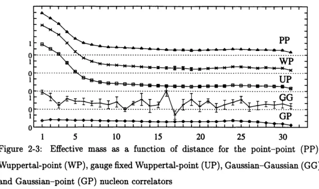
2-3 Effective mass as a function of distance for the point-point (PP), Wuppertal-point (WP), gauge fixed Wuppertal-point (UP), Gaussian-Gaussian (GG) and Gaussian-Gaussian-point (GP) nucleon correlators .... . 30

2-4 Effective m asses ... 32

2-5 Mass it-dependence ... 32

3-1 u and d contributions to t1 for p = (0, 0, 0), n = 0.15200(A),0.15246 (B), 0.15294 (C) . . . . . . . .. .. . 65

3-2 Comparison of t1 calculated with p = (0, 0, 0) and p = (1, 1, 0) . . . . 66

3-3 Extrapolating tl to the chiral limit ... 67

4-1 Topological charge loops ... 71

4-2 The topological charge by intersection counting . ... 74

5-1 Honeycomb domains on the triangular lattice . ... 80

5-2 Parallelogram domains on the triangular lattice . ... 80

5-3 The topological charge distribution p(Q) on the 36 x 12 lattice . . . . 87

5-4 Data for the universal function gt(z) . ... 90

5-5 Data for the universal function gm(z) . ... 90

C-1 An example of plateau search results . ... 100

C-2 x2(S,M)/M for M = 6 ... 101

(10)

(11)

List of Tables

2.1 Conjugate Gradient Inverter . . . .

3.1 3.2 3.3 3.4 3.5 3.6 3.7 3.8 3.9 3.10 3.11

Notations for H4 irreducible representations . . . . Reduction of SO(4) representations to H4 . . . . .

SO(4) to H4: rank 2 ...

SO(4) to H4: rank 3 ...

SO(4) to H4: rank 4 ...

Choice of H4 representations for moments . . . . Moments on the lattice ...

MS renormalization of (9(1) and 0(2) in the continuum. Lattice renormalization of OW(f). ...

Lattice renormalization of 0(2) ...

Lattice renormalization of the tensor charge . . . . .

A.1 Time is in milliseconds for S3 on 32 node VU CM-5 in dedicated mode

C.1

C.2

Result of a gedanken experiment . . . .

min X2(S, M)/M and corresponding S for various M . . . .

. . . . . 40 . . . . . 42 . . . . 43 . . . . 45 . . . . 48 . . . . . 54 . . . . 55 . . . . . 57 . . . . 60 . . . . . 61 .... . . . . 62 95 100 101

(12)

(13)

Chapter 1 Introduction

In this thesis two major topics are described. The first deals with calculation of the hadron structure functions from the first principles. In the second part we develop a novel method of studying topology on the lattice.

Chapter 2 contains an introduction to common lattice techniques. The method-ology of constructing a nucleon on the lattice is also considered there. It ends with establishing the physical scale of the lattice used for the moments calculations in the next chapter.

Twenty years of experimental high energy probes have provided detailed mea-surements of spin-dependent and spin-independent hadron structure functions char-acterizing the distribution of quarks and gluons in the nucleon. Presently, although there is no known way to solve quantum chromodynamics to calculate the structure functions directly from first principles, it is possible to calculate the moments of the structure functions using lattice QCD. The quenched calculations of moments of spin-dependent and spin-inspin-dependent structure functions are considered in chapter 3. The theoretical basis and details of the lattice calculations are described and numerical results for a exploratory calculation are presented.

Since the dynamics of QCD is governed by nonperturbative effects, it is of paramount importance to understand the r61le topological objects play in formation of nucle-ons. An introduction of the 0-term into the Lagrangian calls for special simulation and sampling methods and requires a tremendous increase in statistics to extract a

(14)

signal. While QCD topological effects can not be fully handled by current computa-tional methods, investigation of simpler models is important for better understanding of topology related issues in lattice quantum field theories. Difficulties of previous approaches are reviewed in chapter 4.

Studying the two-dimensional a-model is traditionally a warm-up exercise for nonperturbative QCD. At the same time, it has another application to the behavior of one-dimensional quantum spin chains. Therefore, we develop a method to simulate the 2-d a-model with the 0-term present on a computer in chapter 5. As an application of the technique, we study the mass gap behavior at 0 = 7r.

There are also three appendices in the thesis. In appendix A a portable random number generator is developed for MPP architecture. This implementation has been used in the gauge field generation for chapters 2 and 3. The jackknife procedure for error estimate is summarized in appendix B. Appendix C describes how the plateaux in the experimental data can be determined optimally.

(15)

Chapter 2 Lattice Review

A dream of understanding the properties of strong interactions from first principles is now almost fifty years old. Following the development of quantum chromodynamics in the early 1970's, QCD based calculations of the masses and other properties of hadrons were made possible by Wilson's work on lattice gauge field theory and renormalization group methods. Lattice calculations became a serious player in hadron physics around 1980 with introduction of Monte-Carlo techniques. Since that time, the lattice made its way to the particle physics community, e.g., the Particle Data Book [1] now cites lattice results for a, and the expected glueball mass. Predictions that the 0+ + state is the lightest are now widely believed.

In this chapter we start by reviewing basic lattice concepts and techniques. Sec-tion 2.1 gives the standard set of arguments for using lattice simulaSec-tions to extract nonperturbative results for quantum field theory and introduces the lattice notation. In section 2.2 we construct both gauge and fermion actions suitable for lattice cal-culations. We consider implications of quantum aspects of the theory in section 2.3. Section 2.4 explains how the gauge conditions are implemented on the lattice. The conjugate gradient method of inverting the Dirac matrix is defined in section 2.5. Af-ter that, we show how to construct different hadron sources and discuss their merits in section 2.6. In the last section, 2.7, we establish the scale of the lattice used in the

(16)

2.1 Why Lattice?

Lattice gauge theory goes back to early 70's, when Wilson [2] formulated the lattice theory for regularization purposes. Since that time, lattice calculations developed as a major player in nonperturbative field theory. Currently lattice QCD is widely used to obtain first-principles information about confinement, the hadron spectrum, electro-week decay constants, heavy quark physics etc. In fact, the range of applications is so broad that the proceedings of annual lattice conference is well above 500 pages.

The beauty of lattice field theory is that it allows to study nonperturbative effects while not imposing any ad hoc models. The ambition is to solve QCD from the first principles.

There is yet another appeal to study lattice theories. One can construct and study models which are difficult or impossible to implement experimentally. Besides the Ising model, the 2-d a-model is the most common test model studied by lattice theorists. We will use it in chapter 5 to study 0-vacua.

What all lattice theories share is the departure from continuous 4-dimensional Minkowski space-time we happen to live in. The first steps are to perform a Wick rotation and to replace the flat space-time R4 _{by a manifold M, usually a torus T}4_.

The next step is to substitute a discrete set of points for M.

At this point it is convenient to introduce a notation similar to differential geome-try. This notation works for both finite lattices which can be simulated on a computer and infinite lattices which are useful for analytical calculations.

One way to construct the lattice is to start by dividing a d-dimensional manifold

M into N d-dimensional cells cd(n) without common internal points. This bisection

completely defines the lattice as we shall see presently. If all cells are isomorphic then the lattice is regular, if the cells are of random form, then one has a random lattice. The lower dimensional structures are defined recursively for k = 1 ... d.

A pair of k-cells intersecting over a (k - 1)-dimensional solid define a (k - 1)-cell:

Ck-l(n, m) = ck(n)n ck(m). If one goes on recursively, the last two steps will be

(17)

£ = {{c,}, {cn-1},... {, c},

{o}}

We define a dual d-cell c*(x) as a set of points in

M which are closer to a given co(x) than to any other co. Repeating the previous

procedure one builds the dual lattice £* = {{c*}, {c~_1},.. ., {c*}, {c*}}. This defines

a duality transformation: (ck)* = Cdk. It is easy to see that ((ck(X))*)* = Ck(X), SO

that £** = C.

If the manifold M is orientable, one can introduce the orientation on L.

The boundary operator d maps a k-cell into an oriented collection of (k - 1)-cells forming the boundary of ck(x). E.g., dc, = co(a) - co(b). Analogously, the

coboundary operator maps a k-cell into a collection of oriented (k + 1)-cells: Ock(X) (d((ck (x))*))*

This language closely follows notation of differential geometry (see, e.g, [3]) and shares indeed many advantages of the latter.

One of many choices is to use a torus T4 = R4/Z4 for M and hypercubes for all

Cd. This way we get the conventional QCD lattice. Another discretization will be

used in chapter 5.

The matter fields (scalars, fermions, etc.) live on co: 'Icont(x) --* lat(co). From the differential geometry point of view, the gauge field is a connection, hence it lives on cl defining a parallel transport of the fundamental matter fields along the c1:

A,(x) -- U(cl). In addition, while the continuous gauge field A, was an element of

the Lie algebra, the finite transport U is an element of a corresponding Lie group'.

2.2 Lattice QCD Action

In this section we define the lattice QCD action for both quarks and gluons. From now until chapter 4 we shall work exclusively with 4-dimensional hypercube lattice. It is convenient to introduce another notation for the links and label the link cl (nl, n2, n3)

by the point of origin n and the direction /t: cl -* (n, p). Then the gauge field depends on these two labels: U = U(n, i). The free case A, = 0 corresponds to

U = 1. Occasionally we will label U by a two cos: U(n, it) =- U(n, n + Af).

(18)

The link value can be expressed through A, as follows:

U(n, p) = Pexp IP igA,(x)dx~ ' -) 1 + igaA,(n) + O(a2_).

2.2.1 Gauge Action

To construct a lattice version of the minimal gauge action F2_{, we will need a lattice}

analog to the field strength tensor:

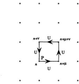
P,,(n) = U(n, n + A) U(n + , n + + ) U(n + + , n + ) U(n + f, n),

(this comes from the definition of the curvature tensor on the principal bundle, see Fig. 2-1.)

n+V U nL+V

n n+U

U

Figure 2-1: Links and a plaquette

In the continuum limit the plaquette becomes:

PI,,(n) ) 1 + iga2F,,(n) - g2a4F,,(n)F,,(n) + O(a6), (2.1)

(There is no summation over it and v on the right hand side). One immediately sees that

P, ( n ) - 1 a- F(n) iga2

Now we need to construct a lattice expression which will reproduce the Lagrange density F, in the continuum. As usual on the lattice, there are many different ways

(19)

to achieve this goal. E.g., -1/g 2_ReTr _,,(P,_{- 1)2} _{is a candidate. However, the} definition of choice of the lattice community is

1

Sglue = Na4g2 _{ReTr (1 - P(n)).} _(2.2)

{CNca 2}

One reason for that will be clear when we discuss lattice simulation techniques. This expression has O(a2) corrections in the continuum limit. Currently there is a lot of

activity on improving the gauge action. (In addition to the perturbative approach of Symanzik [8, 9] there are important recent developments based on the renormalization group [10, 11, 121.)

2.2.2 Fermion Action

For the fermions the situation is more subtle. One can easily write down an expression with a correct continuum limit, e.g.,

Sferm

₂

Z P 7M,U(n, n +

)n+p, -

nyU(n, n

-

)'n-ii

-

am

Z

nn

Cl CO

but there is a notorious fermion doubling problem [13, 14], with the effect that this Lagrangian describes fermions with a wrong number of degrees of freedom. It has been proven that the doubling problem can not be eliminated if only interactions with a finite number of neighbors are considered [15] and both the chiral symmetry and hermiticity are kept intact. In d dimensions the number of doublers is 2d .

Many different approaches were suggested to combat this problem [2, 16]. We will use so-called Wilson fermions:

Sr =

E

, - , _

-

[#x

(R - ytU) U•,,x+, + +x (R + yM) Vut,- - (2.3)

For R - 0, extra degrees of freedom acquire additional mass and are hence pushed out of the massless region. We will use R = 1, because this gives the theory some nice properties in the transfer matrix formalism and considerably simplifies computations. The hopping parameter . replaces the continuum mass. In the free case, U = 1, the Lagrangian (2.3) describes fermions with mass

1- 2d,/

(20)

When the gauge interaction is present, this relation is replaced by

S= q).

_(2.4)

2a K Kc

The renormalization factor Zq depend on the form of the action. For the Wilson action at

f

= 6.2 its perturbative value is close to 1.12 [17, 18]. Kc is the value of the hopping parameter where fermions becomes massless. Its value depends on the dynamics of the gluon sector. The bad news about the Wilson action (2.3) is that in the continuum limit, a -+ 0, R = const, it has order a corrections. This results in the relatively strong r'-dependence of the observables and increases statistics needed for the same accuracy of the extrapolation to the chiral limit compared to the staggered fermions. Furthermore, since there is no remnant on chiral symmetry. the mass is protected against renormalization an the chiral limit requires fin tuning. However, the convenience of the action (2.3) for numerical simulations often outweights its drawbacks. It also simplifies calculating the renormalization constants.

In contrast, although staggered fermions maintain a remnant of chiral symmetry, they only partially remove the doubling problem and strictly apply to integer multiples of 4 flavors. In addition, because of thinning of degrees of freedom, the effective lattice spacing for staggered fermions is actually 2a.

In the next chapter we will use lattice covariant derivatives for fermions:

(0D1 On>

= (V)5

DOn + (0C D1, O),

(2.5)

where

(V) D O)n = On(Un,jVn+A - 'O) (2.6)

and

( D 7)n

=

(On-i!-n',

-

O-)lI"W

(2.7)

2.3 What Makes It Tick

Now, once the action is defined in both fermion and gauge sectors, we can proceed to building the quantum theory on the lattice.

(21)

In general, the way to evaluate the functional integral Z = f[d¢]e-s[0] is to gen-erate an ensemble & of points {(} in configuration space distributed according to the weight p(k) , e-sk[] and use the estimator

E

A[01

a f[dq]A[f]e-S[0l

OE ZZ

for the observable A[¢].

In some cases, it is possible to construct an algorithm producing field configura-tions that are representative of a large number of points in the configuration space so that a part of the sum on the left hand side of the above equation can be done analytically. Such cluster algorithms have been constructed for spin models and gen-eralized to the a-model (we will use cluster updates in chapter 5), but presently there is no efficient construction known for the SU(N) gauge theory.

It is very important that the ensemble & consists of statistically independent configurations and covers the configuration space completely. One method to generate such an ensemble is to use a Markov chain satisfying the detailed balance principle: If

C and C' are two configurations with actions S(C) and S(C') respectively, then the

probabilities to move from C to C' and back (P(C', C) and P(C', C) respectively) must satisfy the condition

P(C', C)e-S(C) = P(C, C')e-_S(C'). _(2.8)

In addition, we require that P(C, C') > 0 for all C, C'. This ensures that any point in the configuration space can be reached by the random walk. Since the walk is defined as a discrete chain of field configurations, it is not required that the configuration space is connected in order for all topological sectors to be automatically sampled in

E with a correct weight.

If we were able to use the whole Markov chain for the estimators, it would be the end of the story. Unfortunately, computers produce only finite sequences of configurations. Thus, the question of statistical independence of the configurations needs to be addressed. Obviously, if two configurations C and C' differ in only small number of variables, then physical observables will be strongly correlated.

(22)

So far, the Markov chain construction does not impose statistical independence on consecutive fields. If the correlation time T of the simulation algorithm is known, then one can build an ensemble of statistically independent configurations by picking up steps from the chain separated by at least r iterations.

One commonly used update algorithm is the heatbath [19] which can be efficiently implemented for the SU(2) Yang-Mills gauge field. Its efficiency is based on the fact that the group manifold is a three dimensional sphere S3 so that a new value of the link can be generated efficiently with the sharp peaked probability exp(-PS(U))dU. Since for SU(N), N > 3 the group manifold is not a sphere any longer and as a result, a straightforward implementation of the heatbath must deal with a sharp peak in the probability distribution. Cabibbo and Marinari [20] suggested a way around this difficulty. Their idea is to use the heatbath for updates in SU(2) subgroups of SU(N). The suggested algorithm automatically satisfies the detailed balance principle (2.8). While it is enough to update only two subgroups (0, 1) and (1, 2) to cover the whole

SU(3), the autocorrelation time is significantly reduced if the third subgroup (1, 3) is

also updated.

Overrelaxation is another method widely used for gauge field generation [21, 22]. It can be considered as a special case of the heatbath algorithm when a new configuration has exactly the same action as the old one. The Wilson action (2.2) considered as a function of one U,•, only can be written as C1 + C2ReTr(UA) where A is

a Nc x N, matrix and Ci are some constants. Again, the SU(2) case is special:

A = kB, B E SU(2) and, e.g., U- > BtUtBt preserves the action (2.2). If Nc > 2 the same Cabibbo-Marinari trick could be applied as for the heatbath.

Simulating the fermion sector of the theory is a separate topic which we shall not discuss here since there are no dynamical fermions in the quenched approximation.

2.3.1 Details of the Field Generation

For calculation of the structure function moments in chapter 3 we generated SU(3) quenched configurations using the Wilson action with 3-subgroup Cabibbo-Marinari interlaced with 16 overrelaxation sweeps on a 243 x 32 lattice. SU(2) subgroups were

(23)

chosen in order (01), (12), (02). First the heatbath algorithm was applied to each subgroup, then 16 overrelaxation sweeps were performed. Each overrelaxation sweep consisted of sequential updates in the same subgroups. Relative numbers of heatbath and overrelaxation iteration were selected based on a tradeoff between autocorrela-tion time (in iteraautocorrela-tions) and run-time of the algorithm. While comprehensive studies of the autocorrelation time is prohibitively expensive, results indicate that using ev-ery 50th iteration for inverting the Dirac matrix and calculating all the observables introduces reasonably small statistical errors due to correlations between the gauge configurations. Moreover, these errors are completely overshadowed by other sources of noise.

The generation started from the cold start (U = 1) and first 7000 iterations were discarded to allow for system thermalization. The coupling constant was held at

p, = 6.2 throughout the simulation.

2.4 Gauge Fixing

In our calculations sometimes2 we need to fix the gauge by imposing some gauge condition G(U) = 0. On the lattice it amounts to finding an extremum of some

func-tional F[U] with respect to gauge transformations g : U(n, m) --+ g(n)U(n, m)gt(m).

The extremum condition for the functional F must reproduce the gauge condition G. Otherwise we are free to use any suitable functional.

2.4.1 Landau Gauge

The Landau gauge 8,A" = 0 corresponds to the functional

3

FL[U]

= E (U (n)

+ U(n))

n A=O

2

Currently we do the gauge fixing for distributed sources only, but it is not difficult to imagine some Dirac matrix inversion method whose convergence would from the gauge fixing also. One such example is Fourier acceleration, for which a smooth gauge like Landau gauge is desirable.

(24)

Finding an extremum of FL[U] requires an iterative procedure, e.g., one may sweep through the lattice maximizing FL [U] with respect to the local gauge transformations. Here again it is advantageous to use the Cabibbo-Marinari trick, since the maximum in SU(2) case can be found by solving an algebraic equation.

2.4.2 Coulomb Gauge

The Coulomb gauge diAi = 0 corresponds to the functional

3

FG[U] = E~~ (U (n) + U (n)) . (2.9)

n i=1

The difference between Landau and Coulomb gauges is in the range of the internal sum over directions. In the Coulomb case it runs over spacial directions only, so that (2.9) admits gauge transformations which depend only on time. It can also be fixed using a procedure similar to that for Landau gauge. The difference from Landau gauge allows to fix the Coulomb gauge in the time slices of interest only. In our case it is enough to fix the Coulomb gauge on the source and the sink time slices instead of fixing it on the whole lattice. We did not use this miniscule optimization for two reasons. First, the time spent in gauge fixing amounts to about 2% of the full computations, and, second, it is simpler to fix the whole lattice once and for all instead of worrying about gauge transforming the propagator when building the two-point function (see section 2.7) and sequential source (section 3.6).

We use the Coulomb gauge when constructing the smeared nucleon sources in section 2.6.

2.4.3 Computation Details

Because of the nature of the functional (2.9) an iterative procedure is needed to find its minimum. A sweep through the lattice consists of changing every link Un,, in such a way that its contribution to (2.9) is minimized.

Applying a gauge transformation at the site n only, the change in (2.9) is

3 3

6FG[U]

=

FG[U

_{]- FG[U]}

9 _{= (g.u,(n)}

_{+ u:(n}

_-)g)

_-

_(U(n)

₊

_t(n

-)

(25)

Since 6FG is linear in g, its minimum can be easily found by cooling methods. In

SU(2) case the group manifold is a sphere and the minimum can be found exactly

by solving a linear equation. In case N > 2 the Cabibbo-Marinari procedure helps again. We used 3 SU(2) subgroups.

Once the gauge transformation minimizing FG locally is found, the same procedure can be repeated on the next site until the entire lattice is swept. Because of the structure of FG one needs to perform multiple sweeps through the lattice before the gauge can be considered fixed.

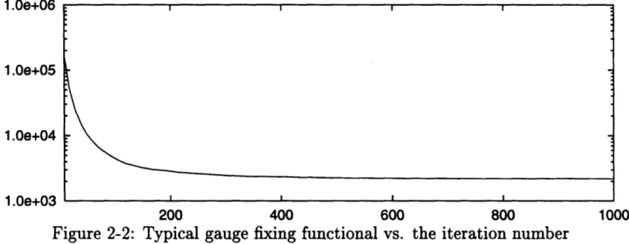
One can also combine the gauge fixing with overrelaxation methods [23, 24]. We did not do it for the present calculations though.

The overall change in FG after one sweep determines how close to the fixed gauge the configuration is brought. Figure 2-2 shows typical behavior of FG as a function of

1.0e+06

1.0e+05

1.0e+04

1.0e+03

200 400 600 800 1000

Figure 2-2: Typical gauge fixing functional vs. the iteration number

the number of iterations. In hadron structure function calculations we fix the gauge before inverting the fermion matrix. The empirical tests show that using 1000 gauge fixing sweeps bring us to the region where results do not noticeably depend on further increasing the number of iterations. Though all observables are gauge invariant, the distributed sources we are using (see section 2.6) are defined in the Coulomb gauge, so ultimately the results do depend on the gauge. One really needs to check the behavior of observables conclude that the gauge has been fixed to the acceptable level, since the functional itself changes very little from iteration to iteration. Notice the logarithmic scale on figure 2-2.

(26)

2.5 Solving the Dirac Equation

Another piece of machinery we need is the fermion propagator in a given gauge field background. In case of the Wilson action (2.3) this amounts to finding an inverse of the matrix:

Ma b(x, Y)= 6xy6,ap 6ab - rZ

{6+,iy

(6oji 7

'ap)

Uab(x, ))+ (2.10)

Ja

(6

8 +

+

&)

U a(X

-

A.,I)

To shorten the notation we will write Mj instead of Ma"(x, y) hereafter. Though thei

matrix M is sparse, with O(N) nonzero elements on a lattice of N sites, its inverse is not. Fortunately, as a rule we not need all N x N elements of M- 1_{, instead we are}

mostly interested in solving the equation

MijSj = qi (2.11)

for a given right hand side q. Before trying to solve this equation, some remarks are due.

First, one notices that (2.10) builds (MO),n from its nearest neighbors only. Hence, if we divide the lattice into even sites (nl + n2 + n3 + n4 = 0 mod 2) and odd sites (nl + n2 + n3 + n4 = 1 mod 2), then one can rewrite (2.11) as

KKoe 1 1o 7o

This system can be immediately solved for one component of 0. E.g., Vo = go

-nKoeO. Then for Pe one has:

MeeCe = ?'e, Mee = 1 - K2KeoK.o, 77 = 77e _- Keo?0o. (2.12) After that we apply the conjugate gradient inverter [25]. Note that since the con-jugate gradient requires a Hermitian matrix, we actually solve the equation MtM¢ =

(27)

€o = 0, 77' = r7_e_{+ IKeorlo, ro =}

_r)'

_- _Mo

0, Po = Mtro Repeat until Irkl is small enough:

SMtrk22 ak - iMpkJ2 0k+1 = Ck + akPk Tk+l = Trk - akMpk

b

trk 12 bk "- Mtrk2 Pk+1 = Mtrk+l + bkPk

Oe

=

€k+1,

'o

= o - IKoek+1

Table 2.1: Conjugate Gradient Inverter

2.6 Sources

Once we have a gauge field configuration we can inhabit it with all kinds of hadrons. Ideally, one would use a creation operator for a given particle. However, the situation is not that simple; since our building blocks are quarks, the detailed knowledge of the quark distribution is needed to create a pure hadron state. By itself this is a problem at least as complicated as, e.g., that of measuring structure functions. What we do instead is construct a source which has large enough overlap with the state of interest and propagate sufficiently far in imaginary time to project onto the ground state. If the source has some quantum numbers fixed (e.g., spin and parity) and the state N we are after is the lowest state with these quantum numbers, then in a few lattice steps all excited states will die off and one can work with N on the rest of the lattice. Of course, at large separation there are considerable fluctuations which make it difficult to pick up the signal from the noise, so in practice the usable region is somewhat limited. The larger overlap of the source with N the better, because it decreases the amplitudes of the higher excitations.

Though the true hadron wave function does not factor into a product of the valence quark wave functions, such a decomposition for the source has several advantages.

(28)

First, it is easy to construct a source with fixed spin, parity and isospin. Second, one can get considerable overlap of a simple source with the lowest state in a sector with fixed (S, P, I).

We start with creating pseudo-scalar mesons. Besides being the simplest color singlets, they are instrumental in determining the lattice scale (see section 2.7.) The following source has IG(JPC) = 1-(0-+):

W')()= -aa (q, x)Y/0Va(q,

x).

Here /(q, x) creates a single quark. We study various choices of

4P

in the next section. For vector mesons, IG(JPC) = 1+(1- -) one can use

IW

(

=

Oaa(q,x)

(qx)

In the baryon sector several sources are widely used. We will use the following lattice operator to create a nucleon

j(N)(x) = a(qi, x) (ql, x) (C75)' (q2, X)abc.

One can easily check that it has I(JP ) = 1/2(1/2+).

In the above formulae, 0 can be a local quark source, Op(q, x) = q(x), or some kind of a smeared distribution which in general can be written as

y(q,

x)

=

d3_yf•b(x,y)q _(y). _(2.13)

Below we consider relative merits of several f(y, z). Section 2.7 shows the relation of

f(x, y) to the right hand side of eq. (2.11).

* Point Source The quark fields are combined pointwise to get the hadron quan-tum numbers. Being a 6-function in space, this operator has extremely large overlap with higher excitations. Depending on the sector, its overlap with the lightest state could become rather small with exited states dominating most of the statistically useful region. This behavior tends to worsen as a - 0.

(29)

* Wuppertal Source Though this source can be written in form (2.13), it is

much more clear to follow the original notation [26]. Using the hopping matrix

3

H(x, x') =

_i=

(ui(X)6 ₁,"X± + U7t(x - )6,_i) I

one defines 0(q, x) = Zx,(1 +aH(x, xz'))q(x'), where q(x) is the quark creation

operator. This source is manifestly gauge invariant. The smearing is controlled by two parameters (a, N).

* Gaussian Source In the Coloumb gauge we define the smeared source with

f'ab(x,

y) = 6ab6a exp(-p(x - y)2). Here p controls the spatial distribution.

* U = 1 Wuppertal Source can be built applying the technique of the Wup-pertal smearing with U = 1 and using the resulting distribution for f(x, y) in the Coloumb gauge. This allows us to compare gauge invariant and gauge fixed sources with the same spatial probability distribution for fermions.

2.6.1 Source Comparison

To determine the most suitable form of the source, we investigated the plateau in the effective mass ln(G(t)/G(t + 1)) for the two point functions for the pion, rho and nucleon sources. To make comparison of different sources meaningful, we used the RMS radius

f

d3xx2(Vb(x))*,a(x)

as a quantitative measure of smearing.

Some comparisons are shown for the nucleon case in Fig. 2-3 for 7 configurations at n = 0.1519. The Gaussian (G) and the two Wuppertal (W & U) sources were adjusted so ( 2 • 6.7a , 0.47fm for each quark field, since this smearing produced the least noisy results in all three cases. For more localized sources the excited states are more prominent, whereas for less localized sources the signal becomes noisier at large distances.

As seen in Fig. 2-3, smearing both the sources and the sink results in substantially noisier behavior than smearing only the source. On the scale of the errors in Fig. 2-3,

(30)

1 5 10 15 20 25 30

Figure 2-3: Effective mass as a function of distance for the point-point (PP), Wuppertal-point (WP), gauge fixed Wuppertal-point (UP), Gaussian-Gaussian (GG) and Gaussian-point (GP) nucleon correlators

there is no significant difference between smeared point sink vs. point source-smeared sink. It is interesting to note that the gauge fixed Wuppertal (U) and gauge invariant Wuppertal (W) sources are essentially equivalent.

The meson sources show similar behavior.

2.7 Lattice Scale

There are two reasons to calculate two-point functions on the lattice. First, it lets us establish the lattice scale from a hadron mass, and we will use the p mass. Second, we will use the two-point function on a given separation to normalize the moments of structure functions from three-point function in chapter 3.

We consider the following two-point function projected onto momentum p:

D2(t, p) = d3xeip(T[J(t, x)J(0)]),

(31)

If J is sufficiently far from the lattice boundary, D2(t) can be written as

D

2

(t, p)

=

I

(OJ(O)n) 1

2e- E(p)t,

after using the Euclidean translation J(t, x) = exp(Ht - ipx)J(O) exp(-Hp + ipx)

and an insertion of a complete set of states 1 = ,n

In)(nl.

This relates the 2-point function to the mass spectrum in the corresponding sector.

One can substitute an explicit form for the hadron creation operator, and, after contractions one gets for the nucleon

D"a'(t,p) f d3_{xeip'( Sa',(x, t;O, to)Sbb (x, t; 0, to)S ,(, t; 0, to)9}

-gb, (X, t; 0, to) b', (X, t; 0, to) gc' (X, t; 0, to))

Eabc a'b'c' (C ₅

)

₇(C ₅

)

₇ '

and for mesons

D2(t, p) =

J

dxe pS~(,( t; 0, to₎ S b(0, to; x, t)F Fa a' ab'6ab'

where we expressed the meson source as jy = a rp•", bab. For the pion F = y•, and

1

= y, for the p meson.

Combining these two expressions for D2(t) the masses of the lowest excited states can be extracted from the t-dependence. A particularly convenient method is to use the effective mass

D2(t)

meff = log

_D

2 (t + 1)'

which asymptotically approaches mo at large distances. Figure 2-4 shows the effective masses for N, p and 7r versus lattice time for 35 (A) and 31 (B) configurations. One can clearly see that the plateau is being reached at fairly short separations of the source and the sink. We used the same set of propagators to determine the lattice scale as for three-point function calculations. The Gaussian smeared source fixed at

x = 0 and point momentum projected sink (p = 0) were used. We estimated errors

using the jackknife procedure outlined in appendix B.

Figure 2-5 shows the quark mass dependence of the nucleon (N), vector (p) and pseudo-scalar (7r) mesons. Observed data agree well with the previously published [27]

(32)

1.0 0.8 0.6 0.4 0.2 0.0 1.0 0.8 0.6 0.4 0.2 0.0 A ---C~f -- as 0 5 10 15 20 25 30 B a.~u~ 0 5 10 15 20 25 30

Figure 2-4: Effective masses at K = 0.15200 (A) and n = 0.15294 (B).

0.70 0.60 0.50 0.40 0.30 0.20 0.10 0.00 0 20 40 60 80 100

Figure 2-5: Mass K-dependence

values of Kc = 0.15329+7 and a- 1 rescaling errors to bring X to 1. explained in appendix C. This fixes

= 2.8GeV. Entries marked with a * indicate

The procedure used to find plateau regions is the scale as follows:

0

mI

, MeV

amN

amp

am,

0.15200 35 86 0.4891(11)* 0.3245(06) 0.2197(04) 0.15246 35 55 0.4442(14) 0.3057(07) 0.1817(04) 0.15294 31 23 0.3552(29) 0.2824(16) 0.1188(08)*

0.15329 0 0.3530(110) 0.2700(80) 0

In this table we used eq. (2.4) for the quark mass with Z = 1.12. In the hadron

(33)

spectroscopy it is generally believed3 that nucleon masses are very unreliable when

m, < 3/La. Our lightest quark mass is presumably too far in that region. Though

both the hadron and mesons have roughly the same RMS radius, the former seems much more affected at the light quark mass. At the moment we do not have an explanation for apparently stable behavior of p and 7r.

(34)

(35)

Chapter 3 Hadron Structure Functions

Hadron physics has enjoyed very dynamic development in recent years. In the be-ginning few experimental data were available, which only allowed study of domi-nant effects. Now, however, with developing experimental techniques in deep in-elastic scattering of leptons, e+e- annihilation and Drell-Yan processes, not only spin-independent functions can be measured experimentally, but the transversity dis-tribution h1(x) and other chiral-odd distributions as well.

The parton distribution functions on the light-cone are important for understand-ing properties of the nucleon in high energy processes for several reasons. First, they are universal in a sense that the same distributions appear in completely different processes, so if one has measured a complete set of distribution functions from exper-iment or calculated them theoretically, then many hadron processes can be predicted. The distribution functions are invaluable for experiments probing physics beyond the standard model, as it allows us to consider a proton beam as a beam of quarks and gluons of known luminosity and thus relate observed cross sections to the fundamental vertices. Second, since the distribution functions depend on the strong interactions only, they can be calculated from the first principles, e.g., by using lattice quantum chromodynamics techniques. Alternatively, they could be used to test our under-standing of non-perturbative methods and hadron structure.

In this chapter we consider calculation of the hadron structure functions on the lattice. Section 3.1 gives a review of structure functions in the continuum. In

(36)

sec-tion 3.2, we consider effects of the broken Lorenz symmetry on the various funcsec-tions of interest. We move to the lattice in section 3.3. Renormalization is considered in section 3.4. One possible implementation on the lattice is described in section 3.5. We study different ways to create the proton on the lattice in section 3.6. Finally, in section 3.7 a calculation of the lowest moment of the tensor charge is presented.

3.1 Moments of Structure Functions I(Continuum)

In this section we summarize relevant continuum operators whose matrix elements will be computed numerically. Where possible we follow the notation of [28] which, in turn, is based on [29, 30, 31].

The forward virtual Compton scattering amplitude is related to the matrix element of the polarized on-shell nucleon (p2 ₌_M2_{, s}2 ₌_{_M} 2 _and_s_-_p₌_{0) state}

T,,(q,p, s) - i f d4 e' (psIT(J, (x)J, (O)) ps) (3.1)

The imaginary part of T,, can be written in terms of various scalar structure functions:

2 ImT, ₁_f _d4_x_eq.

x (p [J,(x), JV(0)] ps)

= -g,, Fi (x, Q2) + PP F(z, Q2)

+iV'IqS gl(x,Q 2 + (s _ p 'qs)g2(X, Q2)] +... +• (3.2)

l] V

where Q2 = -q2 > 0, v = p - q Q2/2 and x = Q2/2v. The normalization of the nucleon state vector is chosen as (pslp's') = (2r)3 2po63(p - p')6s,,,, with

p0 = Ep = /MT

+

p and M being the mass of the nucleon.

In this work, we restrict our attention to the twist-2 structure functions included in eq. (3.2), which are the leading terms in the large Q2 limit.

3.1.1 Spin-Independent Case (F

1

and F

2

)

The moments of the structure functions F1 and F2 are related to the forward

(37)

For even values of n > 2 one has i dx xn - F1 (x, Q2) 2 , C (p2/Q2, g(p)) v($)(p) (3.3) f=u,d

f0

dx

x'Z-

_j

1:

,n

n

(3-4)

d 2 _F 2( 2 = f=u,d C2 ,(f/Q2, g(,))vo/)(p) (3.4)

where the matrix elements v$f) (p) are defined by

I 1 ... ps) = 2v(f) [p, ..p, - traces] (3.5) 81

{12" ... (Y x) 1 D~2 ... D" n} }Of(x) - traces. (3.6) The trace terms in the above equations is needed to construct an irreducible repre-sentation of the Lorenz group. E.g., for n = 2 the right hand side of eq. (3.5) is

PA1P2 - P2/46-,112

The Wilson coefficients c,) (1 2/Q2, g(jL)) and c, (p2/Q2, g(ti)) are known to the

second order in perturbation theory; they can also be computed nonperturbatively on the lattice [32]. Although the structure functions are independent of the subtraction scale, p, the matrix elements and the Wilson coefficients separately do depend on p. In the parton model the moments of F₁ and F2 can be interpreted in the following

way:

v(f) = (x n-)(f) (3.7)

where x denotes the momentum fraction of a nucleon carried by quarks.

3.1.2 _{Spin-Dependent Case (g9 and g2)}

The moments of the structure functions gl and g2 are related to the forward

spin-dependent nucleon matrix elements through the following expressions, derived from OPE.

For even values of n > 0 for gl and n > 2 for g2

dx n gi(x, Q2) = E e(f)(A2/Q2, g())a/)(p) (3.8)

f=u,d

1 _d _n_g

2(xQ2) = 4 [e 2(f(/Q2, g (p)) d ) - -)(f (3.9)

(38)

where the matrix elements af )(p) and d) )(p) _{are defined by}

(PSI O(5,). _{"l'"_A•-_{""}lPS) -n +}1 a) [SM+lsap.n1 4 1 P..p - traces] (3.10)

0(5,f) (i n .•

{(0A12 2(} -

2 )

z)7fY57{

DiD

... D1n} /(Z) - traces

(3.11)

s[a..)

P)

= d(f) [S(sp,₁- sM1p)p2 ... p - traces]

(3.12)

I(5f,)-

(i--

1 4n-+

[a 2 ...} --2 'f(x)7sY7[ D{,A1]D2 "...

D

} ?f(x) - traces (3.13)

where S, symmetrizes indices p," , ,. _{only, Sn+1 symmetrizes indices}a, Pi, ... 7 ,n

and [Ua{pl]p 2 ... t

}

is defined as

0 _{l2n _}

_=.

₌

_n

+

₁

_[O{ii..I}2

- OI{•7A2.,A} + Oa12'An.,} - OA,21...n}) +

]

(3.14)

such that the following decomposition is true

O 1,, 2...,A} = O{,,IA2...An + 1O[a{2]"₂...

An}

(3.15)

As in the spin-independent case, the Wilson coefficients cV()(g 2_/Q2_{, g(A)) (i}₌_{1, 2)} are known to some order in perturbation theory. The lowest moments in the parton model are interpreted as the fraction of the nucleon spin carried by the respective quark flavors:

ao) = 2Au,

aAo) = 2Ad.

(3.16)

3.1.3 Tensor Charge (hi)

The moments of the quark distribution function (rather than the structure function)

hi are related to the forward spin-dependent nucleon matrix elements through the expression, as defined in [33].

j

dx

Xn-

1

_{[hi(x) - (-1)"-~'h(x)] = t$(}

₁

_)(A)

_(3.17)

where the matrix elements t()(ji) are defined by

(39)

(5',) _.7{/1...Ln-(i•n 2

(3.9-)

- ) bf(x)7₅0,7{1, D,,,₂"DO,.}

O(x)

(3.19)

Here again, t(f) (IL) explicitly depends on the subtraction scale p. t•f) (jL) is also called

the tensor charge of the nucleon for flavor f. It is important to note that hi in eq. (3.17) is only meaningful when a subtraction is implied. To relate hi to a physical process (the Drell-Yan process in this particular case), one needs to perform an OPE type of analysis with a given subtraction scheme. In this regard hi is not on the same footing as the structure functions, such as F1, F2, gl and g2 considered earlier.

3.2 Breaking Lorenz Symmetry

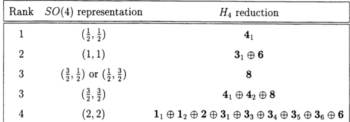
As was mentioned in chapter 2, the Poincard symmetry is explicitly broken on the lattice. In this section we consider the remnants of the rotational subgroup SO(4) that survive on the lattice and the impact of this symmetry breaking on calculations. We start with a condensed review of relevant group theory. For a full treatment of the representation theory of Lie groups and reduction to subgroups, one can use any textbook on the subject, e.g., [34]. We build several low dimensional representations of the hypercubic group H4 and decompose spin 2, 3 and 4 representations of SO(4) into irreducible representations of H4. The results will be used in section 3.3 to construct lattice operators.

H4 is the group of symmetries of the four dimensional hypercube. It has 192 proper

rotations belonging to 13 conjugacy classes. Every element of H4 can be regarded as a product of a permutation of axes and a reflection, with combined parity even. The alternating group S₄acting on the base vectors in R4 _{is a subgroup of H4. On the}

other hand, H4 is a subgroup of SO(4) (the proper rotation group in four Euclidean dimensions), which is locally isomorphic to SU(2) 0 SU(2). Further details and the

representation of H4 can be found in [35].

Let [nin2n3n4] denote a Young diagram of S4 with ni boxes in the first row, n2

boxes in the second row and so on. For example, [4000] and [1111] are the symmetric and antisymmetric representations of S4 respectively. (i,

j)

denotes the spin-i and spin-j representation of SO(4) in the SU(2) 0 SU(2) format. In addition, (i,j) =

(40)

[1111] 0 (i,j). We follow the simplified notation used in [36]. The correspondence with the notation used in[35] is given in Table 3.1.

For our purpose, we need to consider the decomposition of the direct product of

n factors of 41, according to which y, and D, transform under H4, into a direct sum

over the thirteen irreducible representations

n C(H4)

041 = ( ma(n) R

(a)

_(3.20)

i=1 a=l

where R(' ) _{denotes the a-th irreducible representation in Table 3.1 and C(H}

4) = 13

is the number of classes in H4. The integer m, (n) is calculated according to

Table 3.1: The correspondence between notations in references [36] and [35].

m,(n)= D(H4) C _c--1 wx(a)(c)(x(41)(c))n (321)

where D(H4) = 192 is the number of elements in H4, wc is the number of elements

in class c and X(")(c) is the character of the elements of class c in the irreducible representation a.

To explicitly construct the basis vectors which transform as a given irreducible representation, let us introduce the notation lij...), where i,j,... = 1, 2,3, 4. The inner product in this notation is (i'j'... Iij...) = bi 6jj .... The group generators act

on this vector space in the following way. A reflection along the ith axis, Pi, results in a factor of -1 for each index i in I.. .). For example,

P111) = 11), P2121) = -121), P4123) = 123) (3.22) [4000] 1 1 [1111] ₁₂

[2200] 2

[3100] 31

[2110] 32

(1, 0) 33 (0,1) 34

(1, 0) 35

(0,1) 36 (, 2) 41 (1 1) 42 6 6 8 8

(41)

A permutation (ij) interchanges indices with values i and j. For example,

(12)112) = 121), (14)113) = 143), (12)134) = 134) (3.23)

Since reflections Pi and permutations (ij) generate the whole group H4, every group

element can be represented as a finite composition of suitable permutations and re-flections.

3.2.1 Reduction of

SO(4)

to H

4

In general, irreducible representations of SO(4) become reducible when the symmetry is restricted to H4. One can use character orthogonality to find which irreducible

representations of a small group compose a representation of the large group. The relevant formula is

1 C(H4)

m,() = D(H4) c w

X()

C(C)(c) (3.24)

c=1

where (QP)(c) is the character of the SO(4) irreducible representation labeled by 6.

Some of the &( )(c)'s can be found in Table 3.3 of [36]. Others can be calculated by using the SO(4) decomposition rules. For example,

0(2) (1,1) - -

XX'!)!

(3.25)

This equation follows from the SO(4) decomposition (1, 1) (½, 9 ) = (

,

)

E

(2, ) (

(

2)-e,

E,

½),and

V2+ (X(10) + X( °'

₁

) _-

_{2). X.(22}

_(3.26)

from the SO(4) decompositions (1, 0) (, ) = (3, ½) E (½, ½) and (0, 1)

®

(~, ) =

(½, ) E (½, ). In the above calculation, we have used the facts that the SO(4)

representations (0,1), (1,0) and (I, !) are irreducible both in SO(4) and H4, so that ý(c) in these representations are the same. We also used the identity 2(i,) ₌

X(i,O)

.

(O,')

We are mostly interested in reduction of symmetric SO(4) tensors to H4 irre-ducible representations. The results up to rank 4 together with some other useful representations are given in Table 3.2.

(42)

Rank SO(4) representation H4 reduction 1 (½, ₂ ) 41 2 (1, 1) 31 E 6

3 (3, 1) or

(1,

2)

8

3 (, ) 41 e4 2 4 (2,2) 11 e1 2 E 2 E 31

E3

3 E 34 E 35 (3 6 e6

Table 3.2: Reduction of SO(4) representations to H4

While SO(4)-vectors remain irreducible under H4, the higher rank tensors require

more careful considerations.

3.2.2 Rank 2

There are 16 independent vectors Iij), with i,j = 1, 2, 3, 4 in 41 0 41. The decompo-sition

41

0

41 = 11 E 31

E

33 e 34

(

6 (3.27) implies that the rank 2 tensors form five irreducible representations.

orthonormal bases for these representations are as follows:

The explicit

-

(111) + 22)

_{+ 133) + 144))}}

S 1 (3144) 11)

-(122) - |11))}

1 (1[14]) +

1[23])),

=

{ (1

[141) -

[23])),

122) - 133)),

1(2133)

-(3.28)

Ill)

-

22)),

(3.29) (1 [24]) - 1[13])), 1 ([34]) + [12]))} (3.30) S([24])

+

[13])), 1

(I[34])

-

1[12]))}

(3.31)

= {{12}), 1{13}), {14}), 1{23}), 1{24}), 1{34})}

(3.32)

where I[ij]) = (Iij)-Iji))/vý and

I{ij})

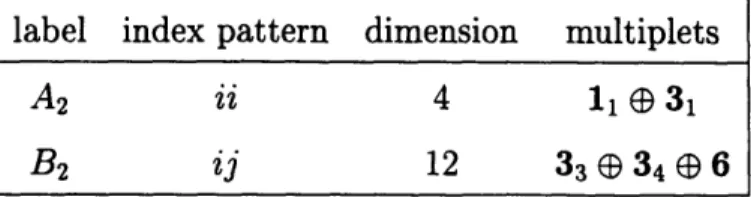
= (lij)+Iji))//- for i # j. The basis vector sets are labeled by their irreducible representations and index patterns according to

(1i•) A2 (31) A2 ý(33) B2 6(34) B2 6(6)_B 2