Aggregate Volatility and Threshold CAPM
Abstract
We propose a volatility-based threshold capital asset pricing model (V-CAPM) in which asset betas change discretely with respect to innovations in aggregate volatility. Using option-implied measures (i.e. returns on at-the-money straddles written on the S&P 500 index and range of the VIX index) as proxies for changes in aggregate volatility, we find that asset sensitivity to market risk changes significantly when aggregate market volatility is beyond a certain threshold. More specifically, portfolios of small (big) and value (growth) stocks have significantly higher (lower) betas at times of high volatility. Due to changes in their market betas, small and value stocks are perceived riskier than their big and growth counterparts in bad times, when aggregate volatility is high. The proposed model also does a better job with pricing, especially for value and small portfolios and when aggregate market volatility is high.
JEL Codes: C24, G12
1. Introduction
Capital asset pricing model (CAPM) assumes that a firm's riskiness, which is captured by its market beta, is constant through time. However, changes in business conditions, technology, and taste might induce shifts in investment opportunity set and investors' associated risk-return tradeoffs. For example, according to Jagannathan and Wang (1996), betas and expected returns vary over time because of changes in the set of firm-specific information available to investors and overall economic conditions. Although there is now considerable empirical evidence on time variation in betas, there is no consensus about how this variation should be modelled. Many studies model the variation in betas using continuous approximation and the theoretical framework of the conditional CAPM.1 However, Ghysels (1998) shows that this approximation fails to capture the true dynamics of betas because of significant structural breaks in parameter estimates. He argues that the actual time variation in betas is slower than assumed by linear factor models such as the conditional CAPM, and advocates the use of the static CAPM until researchers come up with a model that captures the time variation in betas correctly.
In this paper, we model an asset's beta neither as static nor as a continuous approximation implied by conditional models; rather we assume that asset betas change slowly and discretely over time.2 More particularly, we assume that investors update asset betas with respect to changes in aggregate risk conditions, which is captured by innovations to aggregate volatility. There are several reasons why we assume asset betas should change with respect to changes in aggregate volatility. First, although a static CAPM assumes aggregate market risk is constant through time, it is well documented
1
See Harvey (1989), Ferson and Harvey (1991, 1993, 1999), Ferson and Korajczyk (1995), and Jagannathan and Wang (1996) for detailed explanation of conditional asset pricing models.
2
This is intuitively similar to the downside-upside beta approach in Ang, Cheng, and Xing (2006) who show that asset betas change during downside and upside markets and that downside risk is priced. Our approach is also closely related to Markov chain regime switching models, as in Guidolin and Timmermann (2008) and Chen, Gerlach, and Lin (2011).
that equity and aggregate volatility are both time-varying.3 Therefore, an asset pricing model which incorporates time-variation in aggregate volatility would imply that asset betas should change accordingly. Second, economic theory suggests that if investors have mean-variance efficient preferences then they should not only care about market returns but also about innovations to aggregate market volatility. According to Campbell (1993) and Chen (2002), investors are reluctant to lose wealth in periods of high volatility, which represent a deterioration in investment opportunities, and which usually coincides with periods of low consumption (recessions). Thus, assets whose returns correlate positively with innovations in market volatility would be seen as hedges against volatility risk, and would be demanded by risk-averse investors, driving the prices of those assets up, implying lower average returns. In line with this framework, several studies have modelled aggregate volatility risk as a separate risk factor.4 Although our approach takes aggregate volatility risk as the key determinant of the investment-opportunity set, rather than exogenously specifying it as a separate risk factor, we model aggregate volatility as an endogenous parameter, which investors would take into account in determining the riskiness of an asset.
More particularly, we propose a volatility-based threshold CAPM (V-CAPM), where asset betas change contemporaneously with respect to investors' assessment of aggregate risk conditions, which is proxied by changes in aggregate market volatility. The contribution of the proposed V-CAPM is threefold. First, it allows for a slower and discrete variation in betas, as suggested by Ghysels (1998). More specifically, investors do not update asset betas continuously, as in conditional versions of the CAPM, but re-assess an asset's riskiness when aggregate volatility moves beyond a certain threshold. Second, it allows for time variation in aggregate volatility, which is not possible in a static CAPM. By endogenously incorporating aggregate volatility into the CAPM, our model allows betas to change contemporaneously with respect to innovations in
3
For theoretical background and empirical evidence on the stochastic volatility of equity and stock market returns, see French, Schwert, and Stambaugh (1987), Schwert (1989), Engle and Ng (1993), Canina and Figlewski (1993), Braun, Nelson, and Sunier (1995), Andersen (1996), Bollerslev and Mikkelsen (1999), and Bekaert and Wu (2000).
4
aggregate volatility, thus helps better represent changes in the investment opportunity set with respect to changes in aggregate risk conditions. The model is rich in its predictions and offers alternative explanations to some of the empirical failures of the CAPM. Third, we formally test volatility-related regime changes in beta risk, and estimate corresponding betas using Hansen's (2000) threshold regression methodology, which is intuitive and fully supported by econometric theory.5
To test the above hypothesis and to model changes in betas with respect to innovations in aggregate volatility risk, one has to use observable/tradable proxies that best represent investors' information set on aggregate volatility. To do that, we resort to a measure from the options market and use returns on at-the-money (ATM) straddles written on the S&P 500 index as a proxy for aggregate volatility risk.6 There are three main reasons for using ATM straddle returns as proxy for changes in aggregate volatility. First, options provide us with important insights about the underlying spot market. Prices formed in option markets are forward looking and reveal important information about investors’ expectations of the price dynamics of the underlying. For example, the VIX index gives us information about investors’ expectations on the evolution of future volatility in the market, also known as investor sentiment.7 Second, and more important, straddles are volatility trades and their returns are very sensitive to innovations in the volatility of the underlying, making index straddles ideal candidates for examining the effect of aggregate volatility on betas.8 Third, since options themselves are tradable
5
See Hansen (2000) and Akdeniz, Altay-Salih, and Caner (2003) for a detailed explanation of threshold estimation methodology.
6
Another alternative to proxy aggregate volatility would be to use statistical measures such as variance of historical market returns or GARCH-type volatility estimations. We performed similar tests using these statistical measures, however, the results were not significant, confirming our argument that market-based measures do a better job in capturing investors’ expectations on aggregate market risk. Ang et al. (2006), Arisoy et al. (2007), Arisoy (2010), and Cremers et al. (2011) further support the use of option-implied measures as proxies for aggregate volatility risk.
7
VIX is an implied volatility index that measures the market’s expectation of 30-day S&P 500 volatility implicit in the prices of near-term S&P 500 options.
8
Another market-based measure for aggregate volatility risk is the VIX. We also perform our analysis based on a new measure constructed using the VIX index and obtain very similar results. For the construction of this new volatility measure (RVIX) and for related results, the reader is referred to the appendix.
assets, using straddle returns as a proxy for changes in aggregate volatility helps avoid the problem of mimicking portfolios, and helps better represent a dynamically managed portfolio that corresponds to investors’ actual investment opportunity set.
Using returns on S&P 500 ATM straddles as proxy for changes in aggregate volatility risk and portfolios sorted with respect to market capitalizations as test assets, the results can be summarized as follows. First, we document significant time variation in betas. More specifically, nine out of ten portfolios have significant bootstrap p-values at the 1% level, and the modified sup LM test suggested by Hansen (1996) confirms our hypothesis that asset betas change slowly and discretely over time and changes in aggregate volatility is a key determinant in investors' assessment of market risk. Next, we test whether different size portfolios have different beta sensitivities with respect to aggregate volatility risk. Threshold aggregate volatility estimates imply that investors update their beta risk assessments when S&P 500 straddle returns are beyond 15.28% for small stocks and beyond 18.41% for big stocks. Note that index straddles earn positive returns when the market is highly volatile. Therefore, investors update betas depending on whether aggregate volatility is high or low. However, the direction of this change in betas is more striking. Looking at changes in portfolio betas, one can see that stocks in the smallest eight deciles have consistently higher betas at times of high volatility compared to stocks in the biggest market capitalization portfolio. More specifically, small stocks are perceived to be riskier and large capitalization stocks are seen as safer investments at times of high volatility. It is only the stocks in the biggest market capitalization portfolio that correlate less with the market when aggregate market volatility is high. Furthermore, the beta of a portfolio that longs stocks in the smallest decile and shorts stocks in the largest decile (SMB) changes from -0.11 to 0.23, moving from a low-volatility state to a high-volatility state.
We repeat the same procedure for 10 portfolios sorted with respect to book-to-market ratios, and further for twenty-five (5x5) and six (2x3) portfolios sorted with respect to both market capitalizations and book-to-market ratios. The results are similar in that most portfolios exhibit time-variation in betas due to aggregate volatility risk. More particularly, value (growth) portfolios have higher (lower) betas when aggregate volatility
is high, implying that the former are deemed riskier by volatility-averse investors, because their returns correlate more with the market when the market is highly volatile.
French, Schwert, and Stambaugh (1987) and Campbell and Hentschel (1992) empirically document that periods of high volatility usually coincide with downward market moves. Furthermore, risk-averse investors are reluctant to lose wealth in periods of high volatility because this represents a deterioration in investment opportunities, which usually coincides with periods of low consumption (recessions).9 Our findings imply that investors see small and value firms as riskier because their returns correlate strongly with market returns at times of high volatility. On the other hand, big and growth firms are seen as hedges against innovations in aggregate market volatility because their betas correlate less with market returns at those times, implying a higher demand, higher prices, and lower returns. Lettau and Ludvigson (2001) and Petkova and Zhang (2005) also document similar results under conditional CCAPM and CAPM settings, respectively. The authors find that value and small stocks correlate with consumption growth (or market returns) more during bad times relative to big and growth stocks, while the opposite holds during good times. Although similar in spirit, our results imply that investors view small and value stocks riskier than their big and growth counterparts because their returns are more sensitive to market risk at times of high volatility.
To test the power of the above results, we next compare Jensen’s alphas and root mean squared pricing errors of the proposed threshold V-CAPM with those of the static CAPM. In low-volatility states, Jensen’s alphas implied by the V-CAPM are almost as good as the CAPM alphas for most portfolios. However, the biggest improvement in alphas is observed in high-volatility states and especially for small and value portfolios. While the CAPM does a poor job in pricing value and small portfolios at times of high volatility, the V-CAPM alphas are insignificant for small and value portfolios at those times. Furthermore, root mean squared pricing errors for the V-CAPM are always marginally better than those of the CAPM, indicating that the proposed model not only offers a potential explanation to the well-documented size and value anomalies but also does a better job in pricing than the static CAPM.
9
Hsu and Li (2009) document that equity market volatility is higher in bear markets and recessions.
We further test the pricing implications of the proposed model by dividing the sample into high- and low-volatility periods and estimating the corresponding risk premia. Once again, with its significant alpha and insignificant and negative risk premium, the static CAPM is insufficient to explain the cross-section of expected returns throughout the sample period. Looking at the risk premia of the V-CAPM in volatile and calm periods, we find that the market risk premium is still negative and insignificant in low-volatility regime; however, it becomes significant and negative in high volatility regime, implying that investors require compensation for holding stocks that correlate highly with the market when volatility is high. The results are robust to the inclusion of Fama-French factors, SMB and HML.
In order to check the robustness of the results, we extend the sample period to include the recent highly volatile bear market, and introduce an alternative option-based measure, which is the range of the VIX index (RVIX). Following Chou (2005), we define RVIX as the difference between the maximum and minimum levels of VIX in a given month. This results in values of RVIX from January 1986 to March 2010, covering a total of 291 months. We repeat the above tests, this time using RVIX as a proxy for changes in aggregate volatility, and find that the results are robust to the use of an alternative market-based measure and inclusion of the recent volatile period.
The remainder of the paper is organized as follows. Section 2 introduces the threshold V-CAPM and the related econometric framework. Section 3 presents the data and Section 4 documents the empirical findings associated with the proposed model. The final section offers concluding remarks.
2. Threshold Volatility CAPM
To capture the effect of changes in aggregate volatility on market beta, we start with the following conditional CAPM:
1
ri,t1Zt
i tE
rm,t1|Zt
it1,} { 1 1() 1 t zt t x x
where ri,t+1 is the excess return on asset i, rm,t+1 is the excess return on the market
portfolio, and E the expectation operator. t captures time variation in market betas, and
Zt is the conditioning information on investors’ assessments of aggregate volatility risk.
Using returns on S&P 500 at-the-money straddles as a proxy for investors’ information set for changes in aggregate volatility, we model time variation in betas as in Ferson and Harvey (1999). More specifically,
, 1 1{ } 2 { } 1 t t Z Z t
2where 1{} is the indicator function and is the threshold parameter for aggregate
volatility. Combining Equations (1) and (2), we have the following threshold volatility CAPM:
11 21
11{ } 21{ }
, 1 , 1 , 1 ,t Z Z Z Z mt it i r r t t t t
3where Zt is the return on at-the-money S&P 500 straddles that summarizes investors’
information sets on the evolution of aggregate volatility.
2.1 Econometric Model
The observed sample is {rt+1, rm,t+1, Zt}, t = 1, …, T-1. The random variables rt,
rm,t, and Zt are real-valued. The threshold variable Zt is assumed to have a continuous
distribution. Threshold regression has the same format as in Equation (3).
We can rewrite Equation (3) in the following form,
, (4) , = 2, and = 1- 2. where xt+1 = rm,t+1, ) ( 1 1 1 1 t t t t x x e r
The results can further be generalized to the case where only a subset of parameters switches between the regimes and to the case where some regressors only enter in one of the two regimes. Also, takes values in a bounded subset of the real line,
. We assume rmt, Zt, and et are strictly stationary ergodic and -mixing, with -mixing
coefficients satisfying m½ < . The -mixing assumption controls the degree of
time-series dependence, allows the processes to be autocorrelated and heteroskedastic, and is sufficiently flexible to embrace many non-linear time-series processes, including threshold autoregressions.10
2.1.1 Testing for a Threshold
We use the heteroskedasticity-consistent Lagrange Multiplier (LM) test for a threshold, as in Hansen (1996). We test for the null of H0: = 0 against H1: 0.
For all we have the following LM statistics for the null of no threshold:
where is obtained from the restricted least squares. Unfortunately, the large sample limit for the sup-LM test is not nuisance-free because the threshold is not identified under
10
See Hansen (2000) for detailed explanations related to the assumptions.
, ~ ) ( ) ( 1 ) ( V~ , ) ( ) ( 1 ) ( M , ) ( ) ( ~ ) ( ) ( Vˆ , ) ( , ) ( x , ) ( ) ( ) ( ) ( ˆ , ) ( ˆ , ) ( ˆ ) ( ˆ , , 0 , ) ( ˆ ) ( ˆ ) ( ˆ ) ( 2 1 1 * 1 * 1 T 1 * 1 * 1 T 1 1 * T 1 1 * 1 t 1 1 * 1 1 1 * 1 * 1 1 *
t T t t t T t t t T T T t t T t t t T t t t T T e x x T x x T M V M x x r x x x I R where R R V R R T LM t e~the null of no-threshold effect. Because of this issue, Hansen (1996) suggests a bootstrap analog of the suLM test and shows that this method yields asymptotically correct p-values. In this paper, we use the bootstrap analog, following the steps outlined in Hansen (1996).
2.1.2 Estimation
In this section, we estimate the unknown threshold parameter , however, we slightly change the model to have,
(5)
where T is the threshold effect. We let T 0 as T in order to have a nuisance
parameter free asymptotic distribution. However, confidence intervals for can be built even when the threshold effect does not decrease with the sample size. We can rewrite (5) in a matrix form, where X and X are T 2 matrices and R is a Tx1 vector:
. (6) We use the LS estimation:
, ) ( ) ( ) , , ( R X X R X X ST
where ST is the sum of squared errors. To estimate the slope parameters and the threshold
parameter, we observe that first, given , Equation (5) is linear in and T. We can have
the conditional LS estimates by regressing Y on [X X]. Then, set
. ) ), ( ˆ ), ( ˆ ( ) ( T T S S
The estimate of threshold parameter, , can be uniquely defined as,
, min arg ˆ STwhere is minimized over the set T = {Z1,……,ZT}. Therefore, can be derived by
fewer than T function evaluations. The asymptotic distribution for the threshold estimate follows from Hansen’s (2000) Theorem 1.
) ( ˆ and ) ( ˆ T , 1 -T , 1, t , ) ( 1 1 1 1 t T t t t x x e r e X X R T ˆ
3. Data
The market-return data is from Center for Research in Security Prices (CRSP) value-weighted market index for all NYSE, AMEX, and NASDAQ stocks. The risk-free rate is the one-month T-Bill rate obtained from Ibbotson Associates. S&P 500 index (SPX) option data is obtained from Chicago Board Options Exchange’s (CBOE) Market Data Express (MDX). The sample covers the period from January 1987 to March 2007, with a total of 243 months.
The test portfolios consist of stocks sorted according to their market capitalizations and book-to-market ratios. More precisely, we use 10 portfolios sorted according to their market capitalizations, 10 portfolios sorted according to their book-to-market ratios, 10 portfolios sorted according to their dividend yield-to-price ratios, 25 portfolios (5x5) sorted according to size and book-to-market ratios, and six portfolios (2x3) sorted according to size and book-to-market ratios, all of which are downloaded from Kenneth French’s data library.
For proxying aggregate volatility risk, we use the returns on at-the-money straddles written on the S&P 500 index. We construct the ATM straddles as in Coval and Shumway (2001). However, we use standard ATM straddles rather than zero-beta straddles, as those are the volatility trades used by the investors. Before computing the returns on ATM straddles, the following filtering criteria are applied. First, we eliminate all options that violate arbitrage pricing bounds, and the put-call parity by more than 1%. Then, options that expire during the following calendar month are identified, and the options that expire during the next calendar month are used, because they represent the most liquid options among various maturities.11 Options that expire within 10 days are also excluded from the sample because they show large deviations in trading volumes, which casts doubt on the reliability of their pricing.12 Next, each option is checked to determine whether it is traded the next trading day or not. If no option is found in the
11
According to Buraschi and Jackwerth (2001), most trading activity in S&P 500 options is concentrated in the nearest (0–30 days to expiry) and second-nearest (30–60 days to expiry) contracts.
12
nearest expiry contracts, then options in the second-nearest expiry contracts (expiring in two calendar months) are used.
After applying these criteria, we compute daily ATM returns using raw net returns. More specifically, an ATM straddle return is the equally weighted average return on one long call and one put option with strike prices just above the S&P 500 index level, -5 < S-K < 0, and one long call and one put option with strike prices just below the spot price, 0 < S-K < 5. Finally, we cumulate daily ATM returns to monthly returns that form the basis of our tests.
<< Insert Table 1 about here >>
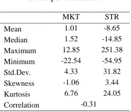
Table 1 reports the summary statistics for the monthly returns on S&P 500 at-the-money straddles (STR), and the market portfolio. For the sample period, S&P 500 ATM straddles on average lost 8.65% per month, which is in line with previous studies. For example, Coval and Shumway (2001) report weekly returns of -3.15% for ATM straddles. Driessen and Maenhout (2006) document weekly returns of -1.67% for the returns on crash-neutral ATM straddles. Broadie, Chernov, and Johannes (2007) report monthly returns of -15.7% for ATM straddles. The correlation between market returns and ATM returns is -0.31.
3.1 Some Stylized Facts
Before moving on to tests of the proposed V-CAPM, this section documents some stylized facts about the chosen threshold parameter, market returns, and the empirically documented size and value vs. growth anomalies.
First, looking at Figure 1, one can see that ATM straddles are indeed volatility trades and they earn huge profits, especially when markets experience significant drops. Second, looking at Table 2, one can observe that size and book-to-market (B/M) portfolios lose more when aggregate market volatility is high. This is in line with Hsu and Liu (2009), who document that volatile periods coincide with bear markets. Third, Table 2 also documents the typical size and value vs. growth anomalies. On average, small
(value) stocks tend to earn higher returns then big (growth) stocks, which is not justified by their CAPM betas. When the sample is divided into calm and volatile periods, one can observe a similar pattern for calm periods. On the other hand, small and value stocks are the worst-performing stocks in volatile markets. Despite their higher average returns, small and value stocks lose considerably at times of high volatility, when the market is doing badly. Furthermore, by losing less than the market portfolio, big and growth stocks offer a partial hedge against volatile market conditions.
<< Insert Figure 1 about here >>
<< Insert Table 2 about here >>
4. Empirical Findings
We begin empirical tests by examining whether there are statistically significant discrete regime shifts in betas due to changes in aggregate volatility risk. Tables 3, 4, and 5 report the associated bootstrap p-values for the sup-LM test. The null hypothesis is that there is no regime shift in portfolio betas. According to Table 3, there have been significant regime changes in betas of most portfolios. For example, for portfolios sorted with respect to market capitalizations, nine out of ten experienced significant changes in their betas during high- and low-volatility periods. On the other hand, for portfolios sorted with respect to book-to-market ratios, the evidence indicates a regime shift in betas of seven out of ten portfolios at the statistical signifance level of 10%. The highest book-to-market portfolio does not exhibit a statistically significant regime shift in betas.
This finding could be due to concentration of high market capitalization firms within the high book-to-market portfolios. The potential existence of big market capitalization stocks in the value portfolios might be driving out the value effect in those portfolios. In order to eliminate this effect and have a clearer understanding of the interaction between size and book-to-market portfolios, we next perform the sup-LM test for 25 portfolios (5x5), sorted with respect to their market capitalizations and book-to-market ratios. As can be seen in Table 4, within the three smallest size quintiles, value
portfolios exhibit significant shifts in their betas between high- and low-volatility regimes. On the contrary, for the two biggest size quintiles, it is only the growth portfolios that exhibit statistically significant p-values. This finding might indicate new evidence and provide an alternative explanation to the empirically observed size and value vs. growth anomalies.
Finally, we refine the sample to six portfolios (2x3) sorted with respect to their market capitalizations and book-to-market ratios. The results for the associated sup-LM tests are reported in Table 5. Consistent with our previous findings, the null hypothesis of no regime shift is rejected for the small-value portfolio. Similarly, the beta of big-growth portfolio exhibits significant regime shifts between high- and low-volatility periods.
<< Insert Table 3 about here >>
<< Insert Table 4 about here >>
<< Insert Table 5 about here >>
The above findings suggest that betas might be stable for size and B/M portfolios during tranquil periods, however, investors seem to update their beta estimates during volatile periods. This is in line with Ghysels (1998), who argues that betas change through time very slowly and the conditional CAPM models may overstate the time variation, and as a result, continuous approximations of the CAPM will produce highly volatile beta estimates. This argument is confirmed with the evidence reported in Braun, Nelson, and Sunier (1995), who use a bivariate EGARCH model to estimate conditional betas and document weak evidence of time variation in conditional betas. According to the V-CAPM introduced here, we document that betas change discretely in time, and this change is determined by changes in aggregate volatility conditions, captured by monthly returns on ATM S&P 500 index straddles in our model.
4.1 The Relationship Between Aggregate Volatility and Beta
Having detected significant regime shifts in betas for most of the portfolios, we proceed to test the magnitude of this change, and estimate market betas and their associated threshold parameters under high and low aggregate volatility regimes. Tables 6 and 7 report the static CAPM betas, betas in low (regime 1) and high (regime 2) volatility regimes, and the threshold estimate for ATM straddle returns, which determines the level of aggregate volatility, above (or below) which investors re-assess a stock’s riskiness.
Panel A of Table 6 documents significant changes in portfolio betas. In particular, betas of stocks in the smallest eight portfolios increase significantly at times of high volatility, whereas the opposite holds for stocks in the biggest decile. This implies that investors re-assess the riskiness of the small market capitalization portfolios when at-the-money straddle returns are above (or below) the threshold of 15.28%. For example, when straddle returns are above 15.28%, investors re-estimate the beta for the smallest portfolio, and update it from 0.87 in low-volatility periods to 1.24 in high-volatility periods. Similarly, the riskiness of the biggest portfolio changes when the ATM straddle returns are above (or below) 18.41%. More specifically, the beta for the biggest portfolio drops from 0.98 in low-volatility periods to 0.93 in high-volatility periods. Furthermore, the beta differential between the smallest and biggest portfolios (SMB) increases from -0.11 in a low-volatility regime to 0.30 in a high-volatility regime. The above results support Campbell (1993) and Chen (2002) findings that investors care not only about market returns but also about innovations to aggregate volatility. Our findings imply that the sensitivity of an asset’s return to changes in aggregate volatility is an important determinant of an asset’s riskiness. This has clear implications for pricing and portfolio allocation. For example, big stocks offer a hedge against innovations to volatility. By having a lower covariance with the market at times of high volatility, which is usually associated with downward market moves and recessions, the biggest portfolio offers a hedge to risk-averse investors, who are reluctant to lose wealth during those times. This implies a demand for big stocks from investors who are averse to innovations in aggregate market volatility, thus pushing their prices up and resulting in lower returns.
Similarly, investors require a premium for holding stocks in small portfolios because they lose much more when aggregate volatility increases. Because increases in aggregate volatility are mostly associated with bad market conditions and deteriorations in investor wealth, by correlating highly with the market at those times, small stocks become much riskier at times when an extra dollar of loss is much more important.
Panel B of Table 6 offers similar results. Five of the portfolios consistently have higher betas at times of high volatility. On the other hand, the two growth portfolios exhibit lower betas during those periods. Although the results are not as strong as those of the size portfolios, the evidence indicates significant time variation in the risk assessments of value and growth portfolios with respect to their sensitivity to changes in aggregate volatility. To better understand the sensitivity of portfolio returns to changes in aggregate volatility, we disentangle the size effect from the value effect by refining the sample in a similar fashion as in the previous section.
<< Insert Table 6 about here >>
<< Insert Table 7 about here >>
Finally, Table 7 reports the beta estimates in low and high volatility regimes, and the threshold parameter estimate for 25 portfolios (5x5) and six portfolios (2x3), sorted with respect to their market capitalizations and book-to-market ratios, respectively. Looking at Panel A, one can see that it is only the two growth portfolios (4-L and B-L) that have lower betas at times of high volatility. Furthermore, it is only the big-growth portfolio which has a beta less than 1 in volatile markets. The remaining portfolios have consistently higher betas in a high-volatility regime, regardless of their book-to-market ratios. Panel B offers similar results. Regardless of being value or growth, small portfolios are riskier in times of high aggregate volatility. However, the increase in risk is most pronounced for the two value portfolios (S-M and S-H). On the contrary, by covarying less with the market in high volatility periods, it is only the growth portfolio among the big market capitalization stocks (B-L) that offers a hedge to investors who are averse to innovations in aggregate volatility. The results are in line with Lettau and
Ludvigson (2001) and Petkova and Zhang (2005), and confirm our previous findings that growth stocks are perceived to be less risky at times of high volatility, whereas value stocks are associated with higher risk at those times.
4.2. Pricing Errors
The documented evidence indicates that asset betas change significantly between volatility regimes. Furthermore, the proposed V-CAPM implies a distinctive pattern in changes in beta risk among different asset classes. More particularly, small market capitalization stocks become riskier at times of high aggregate volatility. The increase in risk is more pronounced for value stocks, and big market capitalization stocks become less risky at those times. A detailed analysis reveals that it is only growth portfolios among big market capitalization stocks that drive this effect. The documented evidence offers an alternative explanation of the well-documented size and value vs. growth anomalies. However, apart from being able to present a relationship between risk and return for different asset classes, a successful asset pricing model should also exhibit lower pricing errors. In order to formally test the improvement gained over the CAPM, we next compare Jensen’s alphas and pricing errors between the static CAPM and the V-CAPM in low- and high-volatility regimes separately.
4.2.1 Comparison of Jensen’s Alphas
Tables 8 and 9 present Jensen’s alphas for different asset classes. Although it performs almost as well as the CAPM, the V-CAPM does not bring any improvement to alphas in the low-volatility regime, regardless of size or book-to-market portfolios. The biggest improvement in alphas comes in the high-volatility regime, especially for value and small stock portfolios. Looking at Panel A of Table 8, one can see that CAPM is unable to explain the returns of the size portfolios in the high volatility regime. On the other hand, the proposed V-CAPM yields insignificant alphas for the 5 smallest decile portfolios and the SMB portfolio. The results are relatively weaker for the book-to-market portfolios, with the only improvement coming for the HML portfolio in volatile
. 2 1 2 , , 1
T t t i t i r r T RMSE periods. Table 9 reveals similar findings for the refined 25 and 6 portfolios. Regardless of asset class, Jensen’s alphas are mostly significant for the proposed V-CAPM, with no improvement over the CAPM during low-volatility periods. However, when the market is highly volatile, Jensen’s alphas for the V-CAPM are insignificant, especially for small-value and big-growth portfolios.
<< Insert Table 8 about here >>
<< Insert Table 9 about here >>
4.2.2 Comparison of Root Mean Squared Errors
In order to check the robustness of the above results, we also calculate the pricing errors of the proposed threshold V-CAPM, as described by Equation (7), and compare them with the pricing errors of the unconditional CAPM and with the Fama and French (1992) three-factor model. The following root mean square error formula (RMSE) is used to calculate the pricing errors of each model:
(7)
In-sample root mean squared pricing errors for each model are reported in Tables 10 and 11, respectively. For the threshold volatility CAPM, we document pricing errors only for portfolios where a significant threshold effect was found. For those portfolios, one can see that the threshold volatility CAPM performs better than the unconditional CAPM in producing lower pricing errors in all portfolios. However, the benchmark 3-factor model yields lower pricing errors compared to the unconditional CAPM and the V-CAPM among all portfolios.
<< Insert Table 10 about here >>
4.3 Risk Premia
There is now considerable evidence about possible time variation in betas, and the conditional CAPM is an attempt to capture this variation. However, Ghysels (1998) shows that the conditional CAPM is unable to specify time variation accurately, leading to higher pricing errors compared to the unconditional CAPM. In view of these findings, we believe that it is crucial to understand the dynamics of time variation in market risk and incorporate this dynamic in the pricing model. Our previous findings establish that market risk exhibits discrete shifts triggered by significant changes in the level of aggregate volatility. Next, we test whether this risk is priced in the cross-section.
We employ standard Fama and MacBeth (1973) two-pass regressions. The full model to be tested is,
) 8 ( 2 , 1 , 0 , , , , , , , j rti i MKTi jMKT j SMBi jSMB j HMLi jHMLj ti
where λ’s represent unconditional prices of risk for various factors, and j=0, 1, and 2 represent the full sample, regime 1 (low volatility), and regime 2 (high volatility), respectively.
More specifically, in the first pass, portfolio betas are estimated from a single multiple time-series using the full sample. In the second pass, a cross-sectional regression is run at each time period, with full-sample betas obtained from the first pass regressions. The associated estimates for the intercept term, αi, and the risk premia, λ’s, are given by
the average of those cross-sectional regression estimates. Table 12 summarizes the risk premium estimates of the model given by Equation (8), or subsets of it.
<< Insert Table 12 about here >>
We test five specifications of Equation (8). The first row represents the market model. Consistent with earlier findings, the CAPM is not a true representation of the pricing kernel of the economy. The market risk premium is negative and insignificant,
and a single factor market model poorly explains the cross-section of returns with an adjusted R2 of 26%. The second row estimates the price of market risk in low volatility regime. Consistent with previous findings, the proposed V-CAPM is not successful in establishing a significant relationship for the price of market risk when market volatility is low. Row 3 estimates the price of market risk in a high-volatility regime. We document a negative and significant market risk premium when the market exhibits high volatility. Previous studies argue that market risk factor is not sufficient to capture sensitivity of stock returns to innovations in volatility. By including volatility risk as a separate risk factor, Ang et al. (2006) and Moise (2007) document a negative price for volatility risk. We show that when markets are divided into low- and high-volatility regimes using our threshold parameter, market risk is able to capture this negative price of volatility risk successfully. Furthermore, an adjusted R2 of 0.40 indicates that the proposed V-CAPM performs much better than the static CAPM in explaining the cross-section of returns in volatile markets.
To see whether the above result is robust we test the proposed V-CAPM in high- and low-volatility regimes with the inclusion of SMB and HML factors, which have been documented as important factors in the literature. Consistent with previous findings the market risk premium of the proposed V-CAPM is still insignificant in calm markets, indicating no improvement over the CAPM at those times. However, Row 5 indicates that negative price for market risk in volatile markets is robust to the addition of SMB and HML factors. Furthermore, Shanken (1992) corrected t-statistics for the intercept term are insignificant, which confirms our previous findings that the proposed model does a good job in pricing, especially at volatile times.
A negative price for market risk at volatile times implies that stocks are expected to have lower returns at those times. Assuming that market is going down at times of high aggregate volatility, stocks with higher betas are expected to lose even more at those times. Thus, agents who are averse to innovations in volatility will demand additional compensation for holding stocks that have high sensitivities to market risk at volatile periods. In other words, a stock whose return correlates highly with market returns at times of high aggregate volatility will be deemed as riskier. To give an example, because of their high betas at volatile times, small stocks are expected to lose 3.13% [4.66 +
1.24*(-6.28)] when the market experiences high volatility. Again, due to differences in their sensitivities to aggregate volatility, a portfolio which longs the smallest decile firms and shorts the biggest decile firms will be expected to lose an additional 1.64% per month [(1.24 - 0.98)*(-6.28)]. Overall, the results imply that the cross-section of stock returns exhibits a negative market risk premium when the market is highly volatile
4.4 Robustness Tests
To test whether the results are sensitive to alternative measures of threshold parameter, we use several statistical and option-based measures as proxies for aggregate volatility. These include the standard deviation of market returns, range of market index (given by the maximum and minimum level of the market index in a given month), GARCH (1, 1) volatility, change in VIX index (ΔVIX), and range of VIX index (RVIX). Among these alternative measures, only RVIX yields significant results and therefore the results of other measures are not reported here.13 Using RVIX defined as the maximum and minimum level of the VIX index in a given month as our threshold parameter, we obtain very similar results to that of S&P 500 ATM straddle returns.14 The results can be summarized as follows.
First, most portfolios exhibit significant bootstrap p-values, indicating a significant change in beta risk due to changes in the range of VIX index, our threshold parameter for aggregate volatility risk. Second, the direction of change is also striking. Similar to previous results, we observe an increase in beta risk for small and value portfolios and a decrease in the risk of big and growth portfolios, confirming our explanation that investors see small and value stocks much riskier at times of high volatility, which usually coincides in deteriorations in investment opportunities and reductions in wealth.
13
This confirms our argument that market-based volatility measures do a better job at capturing investors’ expectations on aggregate market risk compared to statistical measures. Furthermore, Cremers et al. (2011) document that ΔVIX does not capture the volatility risk premium, but ATM straddle returns successfully does.
14
Next, we look at the pricing performance of the proposed V-CAPM and find that it does almost as well as the CAPM, and especially performs much better at times of high volatility and for small and value stocks. Finally, looking at the cross-sectional price of risk, we find that market risk is priced in the cross-section at times of high volatility and is negative.
5. Conclusion
We propose an asset pricing model where the covariance of an asset’s return with the market return changes discretely at different points in time. This change is due to investors’ assessment of aggregate volatility risk. We argue that risk-averse investors care not only about market returns but also about aggregate market volatility while pricing and assessing risk. Proxying aggregate volatility risk first with returns on at-the-money straddles of the S&P 500 index and then with the range of the VIX index, we document the following.
First, we find that there is significant time variation in market betas with respect to changes in aggregate market volatility. In particular, small market capitalization portfolios have consistently higher betas at times of high volatility compared to big market capitalization portfolios. Moreover, the beta dispersion between small and big portfolios is negative during low-volatility periods and positive during high-volatility periods. Because they correlate more with the market, especially at times of high aggregate volatility, small stocks are riskier than big stocks in bad times, when aggregate market volatility is high. Similarly, value portfolios have considerably higher betas significantly at times of high aggregate volatility, indicating that investors perceive value stocks as riskier than growth stocks at those times.
When compared with alternative pricing models, the pricing errors for the proposed threshold V-CAPM are lower than the static CAPM but still higher than those of Fama-French three-factor model. In terms of Jensen’s alphas, the proposed V-CAPM brings the most significant improvement in alphas at times of high volatility and especially for small and value portfolios.
Finally, the proposed V-CAPM cannot establish a significant market risk premium and still suffers from the problems of the static CAPM at times of low market volatility. However, it successfully identifies a negative market price of risk at times of high volatility. The negative price of market risk is robust to the inclusion of SMB and HML factors.
High-volatility periods are usually associated with downward market moves and recessions, i.e. periods when investors are more averse to losing their wealth. Due to their significantly lower betas at times of high aggregate volatility, big and growth stocks offer a potential hedge to investors in bad times. On the other hand, small and value stocks are expected to experience far worse returns when volatility is high. Thus, investors demand big and growth stocks to protect themselves against innovations in volatility. This “flight-to-quality” phenomenon explains why big and growth stocks are generally priced higher and have lower returns, and are seen as less risky compared to their small and value counterparts. The results support the view of a risk-based rational asset pricing theory and offers a volatility-based CAPM where asset return sensitivities to market risk change discretely over time with respect to levels of aggregate volatility.
References
Adrian, T., Rosenberg, J., 2008. Stock returns and volatility: pricing the short-run and long-run components of market risk. Journal of Finance 63, 2997-3030.
Akdeniz, L., Altay-Salih, A., Caner, M., 2003. Time varying betas help in asset pricing: The threshold CAPM. Studies in Nonlinear Dynamics and Econometrics 6, 1- 16.
Andersen, T. G., 1996. Return volatility and trading volume: An information flow interpretation of stochastic volatility. Journal of Finance 51, 169-204.
Ang, A., Chen, J., Xing, Y., 2006. Downside risk. Review of Financial Studies 19, 1191-1239.
Ang, A., Hodrick, R. J., Xing, Y., Zhang, X., 2006. The cross section of volatility and expected returns. Journal of Finance 61, 259–299.
Arisoy, Y. E., Altay-Salih, A., Akdeniz, L., 2007. Is volatility risk priced in the securities market? Evidence from S&P 500 index options. Journal of Futures Markets 27,617-642. Arisoy, Y. E., 2010. Volatility risk and the value premium: Evidence from the French stock market. Journal of Banking and Finance 34, 975-983.
Bekaert, G., Wu, G., 2000. Asymmetric volatility and risk in equity markets. Review of Financial Studies 13, 1–42.
Bollerslev, T., Mikkelsen, H. O., 1999. Long-term equity anticipation securities and stock market volatility dynamics. Journal of Econometrics 92, 75–99.
Braun, P. A., Nelson, D. B., Sunier, A. M., 1995. Good news, bad news, volatility and betas. Journal of Finance 50, 1575–1603.
Broadie, M., Chernov, M., Johannes, M., 2007. Understanding index option returns. Unpublished working paper. Columbia University.
Buraschi, A., Jackwerth, J., 2001. The price of a smile: Hedging and spanning in option markets. Review of Financial Studies 14, 495–527.
Campbell, J.Y., 1993. Intertemporal asset pricing without consumption data. American Economic Review 83, 487-512.
Campbell, J.Y., Hentschel, L., 1992. No news is good news: An asymmetric model of changing volatility in stock returns. Journal of Financial Economics 31, 281-318.
Canina, L., Figlewski, S., 1993. The informational content of implied volatility. Review of Financial Studies 6, 659–681.
Chen, J., 2002. Intertemporal CAPM and the cross-section of stock returns. Unpublished working paper. University of Southern California.
Chen, C., Gerlach, R., Lin, A., 2011. Multi-regime nonlinear capital asset pricing models. Quantitative Finance 11, 1421-1438.
Chou, R., 2005. Forecasting financial volatilities with extreme values: The conditional autoregressive range (CARR) model. Journal of Money Credit and Banking 37, 561-82. Coval, J., Shumway, T., 2001. Expected option returns. Journal of Finance 56, 983-1009. Cremers, M., Halling, M., Weinbaum, D., 2011. In search of aggregate jump and volatility risk in the cross-section of stock returns. Unpublished working paper. Yale School of Management.
Driessen, J., Maenhout, P. J., 2006. The world price of jump and volatility risk. Unpublished working paper, University of Amsterdam.
Engle, R. F., Ng, V. K., 1993. Measuring and testing the impact of news on volatility. Journal of Finance 48, 1749–1778.
Fama, E. F., French, K., 1992. The cross-section of expected returns. Journal of Finance 47, 427-465.
Fama E. F., MacBeth J., 1973. Risk, return, and equilibrium: Empirical tests. Journal of Political Economy 81, 607-636.
Ferson, W. E., Harvey, C. R., 1991. The time variation of economic risk premiums. Journal of Political Economy 99, 385-415.
Ferson, W. E., Harvey, C. R., 1993. The risk and predictability of international equity returns. Review of Financial Studies 6, 527-566
Ferson, W. E., Harvey, C. R., 1999. Conditioning variables and the cross section of stock returns. Journal of Finance 54, 1325-1360.
Ferson, W. E., Korajczyk, R. A., 1995. Do arbitrage pricing models explain the predictability of stock returns? Journal of Business 68, 309-349.
French, K., Schwert, W., Stambaugh, R., 1987. Expected stock returns and volatility. Journal of Financial Economics 19, 3 –29.
Ghysels, E., 1998. On stable factor structures in the pricing of risk: Do time varying betas help or hurt? Journal of Finance 53, 549-573.
Guidolin, M., Timmermann, A., 2008. Size and value anomalies under regime shifts. Journal of Financial Econometrics 6, 1-48.
Hansen, B. E., 1996. Inference when a nuisance parameter is not identified under the null hypothesis. Econometrica 64, 413-430.
Hansen, B. E., 2000. Sample splitting and threshold estimation. Econometrica 68, 575-605.
Harvey, C. R., 1989. Time-varying conditional covariances in tests of asset pricing models. Journal of Financial Economics 24, 289-317.
Hsu, J., Li, F., 2009. Cyclicality in stock market volatility and optimal portfolio allocation. In: Gregoriou, G. N. (Ed.), Stock Market Volatility. Chapman & Hall, Boca Raton, FL.
Jagannathan, R, Wang, Z., 1996. The conditional CAPM and the cross-section of expected returns, Journal of Finance 51, 3-53.
Lettau, M., Ludvigson, S., 2001. Resurrecting the (C)CAPM: A cross-sectional test when risk premia are time-varying. Journal of Political Economy 109, 1238-1287.
Moise, C. E., 2007. Stochastic volatility risk and the size anomaly. Unpublished working paper. Case Western Reserve University.
Petkova, R., Zhang, L., 2005. Is value riskier than growth? Journal of Financial Economics 78, 187-202.
Schwert, G. W., 1989. Why does stock market volatility change over time? Journal of Finance 44, 1115-1153.
Shanken, J., 1992. On the estimation of beta-pricing models. Review of Financial Studies 5, 1-55.
Stoll, H. R., Whaley, R. E., 1987. Program trading and expiration day effects. Financial Analysts Journal 43, 16–28.
Table 1 Descriptive Statistics MKT STR Mean 1.01 -8.65 Median 1.52 -14.85 Maximum 12.85 251.38 Minimum -22.54 -54.95 Std.Dev. 4.33 31.82 Skewness -1.06 3.44 Kurtosis 6.76 24.05 Correlation -0.31
Note: This table reports the descriptive statistics for monthly returns on the market
portfolio (MKT) and S&P 500 at-the-money straddles (STR). The market portfolio is the CRSP value-weighted index for all NYSE, AMEX, and NASDAQ stocks. Monthly returns on S&P 500 ATM straddles are the cumulated daily returns on two equally weighted ATM straddles - one right above and one right below the spot index level. The sample covers the period from January 1987 to March 2007 (243 months). All return figures are given in percentages.
Figure 1
Time-series of S&P 500 ATM straddle returns and market returns
Note: This figure plots the monthly time-series of S&P 500 at-the-money straddle returns (red line, left
axis) and market returns (blue line, right axis) from January 1987 through March 2007 (243 months). The monthly ATM straddle return is the cumulated equally weighted return of call and put options with strike prices just above and below the S&P 500 index and which mature during the next calendar month. The market portfolio is the CRSP value-weighted index for all NYSE, AMEX, and NASDAQ stocks.
-0.4 0.0 0.4 0.8 1.2 1.6 2.0 2.4 -.25 -.20 -.15 -.10 -.05 .00 .05 .10 .15 87 88 89 90 91 92 93 94 95 96 97 98 99 00 01 02 03 04 05 06 07 MARKET STRET
Table 2
Stylized facts about portfolio returns
Panel A: Portfolios sorted with respect to market capitalizations
Size Beta Full
sample Regime1 (Calm) Regime2 (Volatile) Small 0.9705 0.0122 0.0178 -0.0295 Decile2 1.1508 0.0116 0.0176 -0.0330 Decile3 1.1258 0.0119 0.0175 -0.0292 Decile4 1.1241 0.0105 0.0158 -0.0280 Decile5 1.1306 0.0116 0.0165 -0.0248 Decile6 1.0642 0.0108 0.0150 -0.0205 Decile7 1.0486 0.0123 0.0164 -0.0181 Decile8 1.0790 0.0115 0.0154 -0.0169 Decile9 0.9882 0.0115 0.0144 -0.0099 Big 0.9583 0.0099 0.0113 -0.0067 SMB 0.0011 0.0043 -0.0232 Market 0.0101 0.0126 -0.0085
Panel B: Portfolios sorted with respect to book-to-market ratios
B/M Beta Full sample Regime1 (Calm) Regime2 (Volatile) High 0.8690 0.0133 0.0166 -0.0109 Decile2 0.8239 0.0120 0.0141 -0.0034 Decile3 0.7375 0.0112 0.0140 -0.0098 Decile4 0.7754 0.0125 0.0142 -0.0042 Decile5 0.8739 0.0110 0.0136 -0.0081 Decile6 0.8669 0.0114 0.0147 -0.0127 Decile7 0.9239 0.0113 0.0142 -0.0094 Decile8 1.0043 0.0113 0.0138 -0.0077 Decile9 1.0170 0.0102 0.0124 -0.0062 Low 1.0964 0.0098 0.0119 -0.0055 HML 0.0037 0.0034 0.0059 Market 0.0101 0.0126 -0.0085
Note: This table presents the returns on several portfolios that have been used as test assets in this study
and the returns on the market portfolio during the full sample period from January 1987 through March 2007 (243 months) and in two volatility regimes. Size represents portfolios that contain stocks sorted with respect to their market capitalizations. B/M represents portfolios that contain stocks sorted with respect to their book-to-market ratios. SMB is a portfolio that is long in stocks in the smallest decile and short in stocks in the biggest decile. HML is a portfolio that is long in stocks in the highest B/M decile and short in stocks in the lowest B/M decile.
Table 3
Bootstrap p-values for 10 size and 10 book-to-market portfolios
Note: This table reports the bootstrap p-values of the modified sup-LM test suggested by
Hansen (1996). We test the null hypothesis of no significant regime shifts in portfolio betas due to changes in the level of aggregate volatility. STR and RVIX are the threshold parameters. Size represents portfolios that contain stocks sorted with respect to their market capitalizations. B/M represents portfolios that contain stocks sorted with respect to their book-to-market ratios. SMB is a portfolio that is long in stocks in the smallest decile and short in stocks in the biggest decile. HML is a portfolio that is long in stocks that are in the highest B/M decile and short in stocks that are in the lowest B/M decile. Each test is estimated with monthly data from January 1987 through December 2007 (243 months) for the straddle threshold parameter, and from January 1986 to March 2010 (291 months) for the RVIX threshold parameter. *, **, and *** denote significance levels at 10%, 5%, and 1%, respectively. Size STR B/M STR Small 0.001*** High 0.342 Decile2 0.001*** Decile2 0.246 Decile3 0.000*** Decile3 0.067* Decile4 0.000*** Decile4 0.313 Decile5 0.000*** Decile5 0.048** Decile6 0.008*** Decile6 0.005*** Decile7 0.001*** Decile7 0.095* Decile8 0.007*** Decile8 0.093* Decile9 0.253 Decile9 0.057* Big 0.000*** Low 0.092* SMB 0.000*** HML 0.091*
Table 4
Bootstrap p-values for 25 (5x5) size and book-to-market portfolios
Note: This table reports the bootstrap p-values of the modified sup-LM test suggested by
Hansen (1996). We test the null hypothesis of no significant regime shifts in portfolio betas due to changes in the level of aggregate volatility. STR and RVIX are the threshold parameters. Size represents portfolios that contain stocks sorted with respect to their market capitalizations and B/M represents portfolios that contain stocks sorted with respect to their book-to-market ratios. HMLs is a portfolio that is long in stocks in the smallest size and highest B/M quintile and short in stocks in the smallest size and lowest B/M quintile. SMBh is a portfolio that is long in stocks in the smallest size and highest B/M quintile and short in stocks in the biggest size and highest B/M quintile. Each test is estimated with monthly data from January 1987 through December 2007 (243 months) for the straddle threshold parameter, and from January 1986 to March 2010 (291 months) for the RVIX threshold parameter. *, **, and *** denote significance levels at 10%, 5%, and 1%, respectively. Size B/M STR S L 0.019** S 2 0.000*** S 3 0.000*** S 4 0.000*** S H 0.000*** 2 L 0.154 2 2 0.000*** 2 3 0.000*** 2 4 0.000*** 2 H 0.001*** 3 L 0.331 3 2 0.002*** 3 3 0.019** 3 4 0.025** 3 H 0.042** 4 L 0.030** 4 2 0.010** 4 3 0.020** 4 4 0.188 4 H 0.294 B L 0.025** B 2 0.248 B 3 0.292 B 4 0.108 B H 0.628 HMLs 0.068* SMBh 0.007***
Table 5
Bootstrap p-values for 6 (2x3) size and book-to-market portfolios
Size B/M STR S L 0.015** S M 0.000*** S H 0.000*** B L 0.029** B M 0.228 B H 0.335 HMLs 0.063*** SMBh 0.001***
Note: This table reports the bootstrap p-values of the modified sup-LM test suggested by
Hansen (1996). We test the null hypothesis of no significant regime shifts in portfolio betas due to changes in the level of aggregate volatility. STR and RVIX are the threshold parameters. Size represents portfolios that contain stocks sorted with respect to their market capitalizations and B/M represents portfolios that contain stocks sorted with respect to their book-to-market ratios. HMLs is a portfolio that is long in small-value and short in small-growth stocks. SMBh is a portfolio that is long in small-value and short in big-value stocks. Each test is estimated with monthly data from January 1987 through December 2007 (243 months) for the straddle threshold parameter, and from January 1986 to March 2010 (291 months) for the RVIX threshold parameter. *, **, and *** denote significance levels at 10%, 5%, and 1%, respectively.
Table 6
Threshold estimates for 10 size and 10 book-to-market portfolios Panel A: 10 size portfolios
CAPM Beta Beta for Regime 1 Beta for Regime 2 Threshold Estimate
Small 0.9705 0.8716 1.2439 0.1528 Decile2 1.1508 1.0682 1.1959 0.1528 Decile3 1.1258 1.0323 1.2117 0.1528 Decile4 1.1241 1.0299 1.2232 0.1528 Decile5 1.1306 1.0546 1.2055 0.1528 Decile6 1.0642 1.0001 1.1374 0.1528 Decile7 1.0486 1.0001 1.1052 0.1841 Decile8 1.0790 1.0517 1.1001 0.1841 Decile9 0.9882 - - - Big 0.9583 0.9817 0.9396 0.1841 SMB 0.0122 -0.1101 0.3035 0.1528 Panel B: 10 B/M portfolios
CAPM Beta Beta for Regime 1 Beta for Regime 2 Threshold Estimate
High 0.8690 - - - Decile2 0.8239 - - - Decile3 0.7375 0.6261 0.9850 0.0467 Decile4 0.7754 - - - Decile5 0.8739 0.7565 0.9754 -0.0515 Decile6 0.8669 0.7850 1.0020 0.3444 Decile7 0.9239 0.8137 1.0398 -0.0111 Decile8 1.0043 0.9358 1.1332 0.1344 Decile9 1.0170 1.1055 0.9852 -0.1842 Low 1.0964 1.1307 0.9572 0.5553 HML -0.2274 -0.3195 0.0667 0.7956
Note: This table reports the unconditional CAPM betas, the threshold beta estimates with respect to low-
and high-volatility regimes, and their associated threshold volatility estimates, proxied by S&P 500 at-the-money straddle returns. Panels A and B present results for portfolios sorted with respect to market capitalizations, and book-to-market ratios, respectively. SMB is a portfolio that is long in stocks in the smallest decile and short in stocks in the biggest decile. HML is a portfolio that is long in stocks in the highest B/M decile and short in stocks in the lowest B/M decile. The sample covers the period from January 1987 to December 2007 (243 months). Regime 1 (2) corresponds to low- (high-) volatility regimes where monthly S&P 500 ATM straddle returns are lower (higher) than the estimated threshold. Threshold betas and their associated threshold volatility estimates are not reported for portfolios that do not exhibit significant regime shifts.
Table 7
Threshold estimates for 25 (5x5) and 6 (2x3) size and book-to-market portfolios Panel A: 25 (5x5) portfolios
Size B/M CAPM Beta Beta for Regime 1 Beta for Regime 2 Threshold Estimate
S L 1.4372 1.4187 1.4525 0.1528 S 2 1.1566 1.1136 1.1655 0.1528 S 3 0.9521 0.8024 1.0944 0.0197 S 4 0.8770 0.7580 1.0160 0.1528 S H 0.9044 0.7993 1.0051 0.5553 2 L 1.4339 - - - 2 2 1.1062 0.9871 1.2433 0.1528 2 3 0.9223 0.7901 1.0852 0.1528 2 4 0.8812 0.7383 1.0537 0.1080 2 H 0.9697 0.9520 1.0180 0.7956 3 L 1.3500 - - - 3 2 1.0717 0.9667 1.2212 0.1398 3 3 0.8880 0.7736 1.0403 0.1080 3 4 0.8276 0.6988 1.0035 0.1080 3 H 0.8879 0.7866 0.9807 0.7956 4 L 1.2735 1.2904 1.2374 -0.0261 4 2 1.0038 0.8886 1.1618 0.1001 4 3 0.9325 0.8408 1.0641 0.1398 4 4 0.8280 - - - 4 H 0.8453 - - - B L 1.0307 1.0606 0.9624 0.5553 B 2 0.9412 - - - B 3 0.8477 - - - B 4 0.7067 - - - B H 0.7987 - - - HMLs -0.5328 -0.6421 -0.2521 0.5029 SMBh 0.1057 -0.0143 0.2046 0.0367 Panel B: 6 (2x3) portfolios
Size B/M CAPM Beta Beta for Regime 1 Beta for Regime 2 Threshold Estimate
S L 1.3565 1.3110 1.3522 0.1537 S M 0.9540 0.8292 1.1100 0.1537 S H 0.9031 0.7648 1.0691 0.1119 B L 1.0518 1.1066 0.9417 0.5591 B M 0.8504 - - - B H 0.7781 - - - HMLs -0.4534 -0.5502 -0.2177 0.5029 SMBh 0.1250 -0.0415 0.1948 0.0367
Note: This table reports the unconditional CAPM betas, the threshold beta estimates with respect to low- and
high-volatility regimes, and their associated threshold volatility estimates, proxied by S&P 500 at-the-money straddle returns. Panels A and B present results for 25 (5x5) and six (2x3) portfolios sorted with respect to market capitalizations and book-to-market ratios, respectively. HMLs is a portfolio that is long in small-value and short in small-growth stocks. SMBh is a portfolio that is long in small-value and short in big-value stocks. The sample covers the period from January 1987 to December 2007 (243 months). Regime 1 (2) corresponds to low- (high-) volatility regimes where monthly S&P 500 ATM straddle returns are lower (higher) than the estimated threshold. Threshold betas and their associated threshold volatility estimates are not reported for portfolios that do not exhibit significant regime shifts.