Detailed Study of the Decay $\Lambda_b \to \Lambda_c \tau {\bar \nu}_{\tau}$

Detailed Study of the Λ

→ Λ

τ ¯

ν

Decay

E. Di Salvo

, F. Fontanelli

and Z. J. Ajaltouni

a _{Laboratoire de Physique de Clermont - UCA}

4 Av. Blaise Pascal, TSA60026, F-63178 Aubi`ere Cedex, France

b _{Dipartimento di Fisica Universit´a di Genova}

Via Dodecaneso, 33, 16146 Genova, Italy

c _{I.N.F.N. - Sez. Genova,}

Via Dodecaneso, 33, 16146 Genova, Italy

Abstract

We examine in detail the semi-leptonic decay Λb → Λcτ ¯ντ, which may confirm previous

hints, from the analogous B decay, of a new physics beyond the standard model. First of all, starting from rather general assumptions, we predict the partial width of the decay. Then we analyze the effects of five possible new physics interactions, adopting in

each case five different form factors. In particular, for each term beyond the standard model, we find some constraints on the strength and phase of the coupling, which we combine with those found by other authors in analyzing the analogous semi-leptonic

decays of B. Our analysis involves some dimensionless quantities, substantially independent of the form factor, but which, owing to the constraints, turn out to be strongly sensitive to the kind of non-standard interaction. We also introduce a criterion

thanks to which one can discriminate among the various new physics terms: the left-handed current and the two-higgs-doublet model appear privileged, with a neat preference for the former interaction. Lastly, we suggest a differential observable that

could, in principle, help to distinguish between the two cases. PACS numbers: 13.30.Ce, 12.15.-y, 12.60.-i

1_{disalvo@ge.infn.it} 2_{fontanelli@ge.infn.it} 3_{ziad@clermont.in2p3.fr}

1

Introduction

The high energy physicists have been looking for physics beyond the standard model (SM) for some decades. This research has recently received a new impulse from the Higgs discovery[1, 2] and from the data of the semi-leptonic decays B → D(∗)τ ντ[3-8] and

B → K∗`+<sub>`</sub>−_{[9, 10]}4_{, which have exhibited strong tensions with the SM predictions[11-13].}

Indeed, the SM entails lepton flavor universality (LFU), which seems to be contradicted by the measurements of the observables

R_D(∗) = B(B → D(∗)_{τ ¯ν} τ) B(B → D(∗)<sub>`¯ν</sub> `) and RK∗ = B(B → K∗_µ+_µ−₎ B(B → K∗_e+_e−₎. (1)

It is important to notice that these quantities attenuate the biases related to the experimental efficiency, to the values of CKM matrix elements Vcb and Vsb and to the

theoretical uncertainties of the form factors (FF); therefore they appear especially suitable for singling out new physics (NP) effects.

In the present article, we are mainly concerned with the experimental results of the B → D(∗)τ ντ decays, about which some authors have performed model independent

analyses[14-23], while other people have interpreted them in terms of specific NP models, like two-higgs-doublet[24-27] (2HD), leptoquark[14,28-34] (LQ), left-right symmetric[35, 36] (LR) or extra-dimension[37] model. The anomaly has been connected to the leptonic B and Bc decays to τ ¯ντ[24-27,35] and a new light has been cast on the muon anomalous

magnetic moment[27, 32] (see also ref. 38).

All that is a goad to further searches for confirmations of NP. In this sense, the Λb

decays to Λ`+<sub>`</sub>−_{[39, 40] and to Λ}

cτ ντ[41-47], as well as the decays Bc→ J/ψ(ηc)τ ντ[48],

could give definitive confirmations of NP, in particular of LFU violation (LFUV); indeed, these presumably share the same basic processes as the two above mentioned B decays. In the present paper, we consider the baryonic decay

Λb → Λcτ−ν¯τ, (2)

to which a previous letter[45] has been dedicated. Here we give a more in-depth, model independent analysis of this decay, which we compare to the Λb → Λc`ν` one. Precisely,

we limit ourselves to the spin-independent observables and analyze the NP dependence of suitable dimensionless ratios, among which, analogously to (1),

RΛc =

B(Λb → Λcτ ¯ντ)

B(Λb → Λc`¯ν`)

. (3)

To this end, we propose for the NP interaction five different dimension 6 operators, chosen according to the most frequently used models - typically, the above mentioned 2HD, LQ or LR - and similarly to other model independent analyses[41, 43, 47]. The main differences with the previous studies consist of imposing more stringent constraints

on the NP effects, also by taking into account some analyses of the semi-leptonic B decays[15, 19, 17], and of introducing a particular criterion for discriminating among the different NP interactions. Moreover, in order to probe the FF dependence of our predictions, we consider five different alternatives. We find that, while the partial decay width depends rather strongly on the FF, the above mentioned ratios depend much more mildly on them. On the contrary, our prediction about RΛc is quite different from the one

of the other authors[49-56]. However, as we shall see, there are reasons for assuming that the rest of the analysis is independent of this discrepancy. As a last subject, we single out a differential observable which allows, in principle, to distinguish between two of the most likely NP interactions.

Sect. 2 resumes our assumptions, including the above mentioned criterion. In sect. 3, we deduce, in the covariant formalism, the general formulae for the matrix elements; we also introduce the various FF, for which we give a short review of previous contributions. In sect. 4, we sketch the expressions of the differential and partial widths of the decays of interest. In sect. 5, we show predictions of the partial decay widths, both according to the SM and to our assumptions about NP. Sect. 6 is devoted to illustrating the constraints on the various NP couplings. Sect. 7 is dedicated to a discussion of our results, in light our criterion, and to a review of previous analyses. In sect. 8, we exhibit the predictions of the differential decay widths according to two different NP interactions, suggesting a new observable, sensitive to the differences between them. Lastly, some conclusions are presented in sect. 9

2

Assumptions

We list here our assumptions, five in all. The first four are shared by the other authors, whereas the fifth one is the above mentioned criterion.

1) The NP process entails LFUV, therefore it does not act on τ in the same way as on the light leptons. In a simplifying assumption, the NP does not concern at all the electron and the muon.

2) The basic process that gives rise to the NP in the semi-leptonic decays (2) and B → D(∗)_{τ ν}

τ consists uniquely of b → cτ ντ and does not involve any spectator

partons. This is a consequence of the short range of the would-be NP interaction, whose intermediate boson is estimated to have a mass of order 1 T eV [23, 29, 34, 57]. As we shall see, this has important consequences.

3) Only one type of interaction − scalar, vector, etc. − is present in the effective lagrangian.

4) The double ratio

Rratio_Λc = RΛc/R

SM

Λc (4)

depends only mildly on the FF. This assumption is supported by the analyses relative to the semi-leptonic Λb[41, 46] and B[3-8,28,29] decays. In particular, according to refs. 28

and 58, it results

Rratio_D = Rexp_D /RSM_D = 1.30 ± 0.17, R_Dratio∗ = Rexp_D∗/RSM_D∗ = 1.25 ± 0.08, (5)

quite compatible with each other. Further arguments will be exposed below.

5) Lastly, given the reliability of the SM at present energies, the NP term is only a perturbation of the known amplitude for the decay considered. Therefore, we privilege the interactions whose effective couplings are much smaller than the Fermi constant, G = 1.166379 · 10−5GeV−2.

Taking into account the more restrictive of the results (5), the first four assumptions imply immediately that

RΛc = ξ ΓSM τ ΓSM ` , ξ = 1.25 ± 0.08. (6)

Here Γτ (`) is the partial width of the decay Λb → Λcτ−ν¯τ(`−ν¯`); according to our

prediction, Γτ results to be

Γτ = ξΓSMτ . (7)

3

Matrix Element of the Decay

3.1

SM and NP Amplitudes

We consider the matrix element for the decay Λb → Λc`¯ν`5. To this end, we set, in quite

a general way, M = Vcb G √ 2(J L µjµ+ grI). (8)

Here I is the NP interaction and

gr = xeiϕ (9)

the corresponding relative coupling[41], with x and ϕ real, x > 0. We consider five types of effective dimension 6 operators, according to the most frequently used models:

I = JL µj µ_{, J}R µj µ_{, J}S_{j, J}P_{j, J}H_{j. (10)} Here jµ = u¯`γµ(1 − γ5)v, j = ¯u`(1 − γ5)v, (11) J_µL(R) = hΛc|¯cγµ(1 ∓ γ5)b|Λbi, JS = hΛc|¯cb|Λbi, (12) JP = hΛc|¯cγ5b|Λbi, JH = JS− JP (13)

and u` and v are the four-spinors of the charged lepton and of the anti-neutrino

respectively; lastly, L, R, S, P and H denote, respectively, left-handed vector, right-handed vector, scalar, pseudo-scalar and S − P -interaction.

3.2

Form Factors

The most general expressions of the vector and axial hadronic currents are

hΛc|¯cγµb|Λbi = u¯fVµui = ¯uf(f1γµ+ f2iσµνqν + f3qµ)ui, (14)

hΛc|¯cγµγ5b|Λbi = u¯fAµγ5ui = ¯uf(g1γµ+ g2iσµνqν + g3qµ)γ5ui. (15)

Here the fi and the gi (i = 1,2,3) are functions of q2, ui(f ) the four-spinor of the initial

(final) baryon,

q = pi− pf = p`+ p (16)

and pi(f ), p` and p are, respectively, the four-momenta of the baryons, of the charged

lepton and of the anti-neutrino.

Using the equations of motion (eom), the operators Vµ and Aµ, which appear in Eqs.

(14) and (15), can be re-written as (see Appendix A)

Vµ = X0γµ+ f2Pµ+ f3qµ, Aµ = Y0γµ+ g2Pµ+ g3qµ, (17)

where

X0 = f1− (mi+ mf)f2, Y0 = g1+ (mi− mf)g2, P = pi+ pf (18)

and mi(f ) is the mass of the initial (final) baryon: mi = 5.619 GeV , mf = 2.286 GeV .

Moreover, as regards the (pseudo-) scalar current, still, the eom imply[45] JS = q µ δmQ ¯ ufVµui, JP = −ρ qµ δmQ ¯ ufAµui, (19) with δmQ = mb− mc, ρ = mb− mc mb+ mc ∼ 0.53, (20)

mb = 4.18 GeV and mc = 1.28 GeV being the masses of the b- and c-quark respectively.

3.2.1 A Short Review

Different techniques have been adopted for determining the FF for the decay (2): - lattice calculation[49, 47], approximated by an analytical expression[43];

- quark models: constituent[50], covariant[51], diquark[52] and heavy quark Isgur-Wise[53, 54] (IW) model;

- sum rules (SR), both in pole approximation[55, 41, 46] and in full QCD[56]. 3.2.2 Present Analysis

The five different FF we use here are based on some approximations, generally accepted for the heavy quark transition b → c[55]:

Table 1: The four different FF inferred from sum rules: f1is dimensionless, f2 is expressed

in GeV−1 and q2 in GeV2.

SR1 SR2 SR3 SR4

f1(q2) 6.66/(20.27 - q2) 8.13/(22.50 - q2) 13.74/(26.68 - q2) 16.17/(29.12 - q2)

f2(q2) -0.21/(15.15 - q2) -0.22/(13.63 - q2) -0.41/(18.65 - q2) -0.45/(19.04 - q2)

In particular, the first FF is of the IW type[53] and the remaining four are based on the SR[55, 41, 46]. The IW FF reads as

f1(q2) = ζ0[ω(q2)] = 1 − 1.47[ω(q2) − 1] + 0.95[ω(q2) − 1]2, (22) ω(q2) = m 2 i + m2f − q2 2mimf ; f2(q2) = 0. (23)

Incidentally, it is worth noticing that this is quite compatible with the bounds determined by the recent analysis of Λb → Λcµνµ data[54].

The parametrizations of the SR FF are reported in Table 1.

4

Decay Width

4.1

Derivation of Basic Formulae

The observables that we study in this paper are derived from

dΓ = 1

2mi

X

|M|2_{dΦ. (24)}

Here dΦ is the phase space and the symbol P denotes the average over the polarization of the initial baryon and the sum over the polarizations of the final particles. We have

X |M|2 = |Vcb|2 G2 2 [TSM+ 2x<(TIe −iϕ ) + x2TN]. (25)

Here TSM is the SM contribution,

TSM =

X

Hµν`µν, Hµν = JµLJ L∗

ν , `µν = jµjν∗. (26)

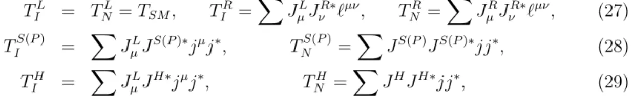
As to the terms TI and TN, they correspond, respectively, to the interference between

the SM and the NP amplitude and to the modulus square of the NP amplitude. Specifically, we have T_IL = T_NL = TSM, TIR = X J_µLJ_νR∗`µν, T<sub>N</sub>R=XJ<sub>µ</sub>RJ<sub>ν</sub>R∗`µν, (27) T_IS(P ) = XJ_µLJS(P )∗jµj∗, T_NS(P ) =XJS(P )JS(P )∗jj∗, (28) T_IH = XJ_µLJH∗jµj∗, T_NH =XJHJH∗jj∗, (29)

the upper indices denoting the various NP interactions.

In the present paper we are not concerned with spin, therefore we consider an unpolarized initial baryon. A standard calculation in the covariant formalism leads to

TSM = 25{(X0+ Y0)2h1+ (X0 − Y0)2h2+ (Y02 − X02)h3

+ A[mf(X0+ Y0)Li+ mi(X0− Y0)Lf] + A2pf · pi LP}, (30)

where A is defined by the second Eq. (21) and

h1 = pf · p` pi· p, h2 = pf · p pi· p`, h3 = mimf p · p`, (31)

Li(f ) = pi(f )· p` P · p + pi(f )· p P · p`− pi(f )· P p · p`, (32)

LP = 2p`· P p · P − P2 p · p`. (33)

As regards the remaining terms, one has T_IR = 26{(X2 0 − Y 2 0)(k1+ k2) − (X02+ Y 2 0)k3 + A[mf(X0+ Y0)Li+ mi(X0− Y0)Lf] + A2mfmiLP}, (34) T_NR = 25{(X0− Y0)2k1 + (X0+ Y0)2k2+ (Y02− X 2 0)k3 + A[mf(X0+ Y0)Li+ mi(X0− Y0)Lf] + A2pf · piLP}, T_IS = 25 ml δmQ [X₀2(k1+ k2) + AX0(k3+ k4) + A2p · P q · P k+], (35) T_NS = 24 pl· p (δmQ)2 [X₀2(k5+ k6) + AX0(k7+ k8) + A2(q · P )2 k+], (36) T_IP = 25 ml δmQ [Y₀2(−k1+ k2) + AY0(k3− k4) − A2p · P q · P k−], (37) T_NP = 24 pl· p (δmQ)2 [Y₀2(k5− k6) + AY0(−k7+ k8) + A2(q · P )2 k−], (38) T_IH = T_IS+ ρT_IP, T_NH = T_NS+ ρ2T_NP. (39) Here k1 = p · pf q · pi+ p · pi q · pf − p · q pf · pi, k2 = mimf p · q, (40) k3 = mi(p · pf q · P + p · P q · pf), k4 = mf(p · pi q · P + q · pi p · P ), (41) k5 = 2q2 pf · q pi· q pi· pf, k6 = mimf q2, (42) k7 = mi pf · q P · q, k8 = mf pi· q P · q, (43) k+ = pi· pf + mimf, k−= pi· pf − mimf. (44)

4.2

Differential and Partial Decay Width

The integration over the phase space is suitably performed by fixing a reference frame at rest with respect to Λb; to this end, it is also worth recalling the relation of q2 to the

energy Ef of the final baryon in that frame:

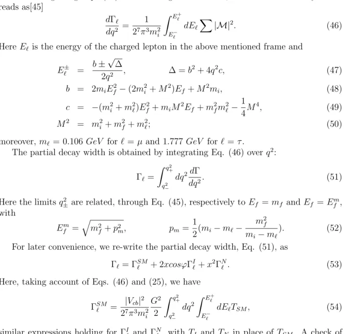
After integrating Eq. (24) over the angular variables, the differential decay width reads as[45] dΓ` dq2 = 1 27<sub>π</sub>3<sub>m</sub>2 i Z E<sub>`</sub>+ E<sub>`</sub>− dE` X |M|2_{. (46)}

Here E` is the energy of the charged lepton in the above mentioned frame and

E_{`</sub>± = b ± √ ∆ 2q2 , ∆ = b 2<sub>+ 4q</sub>2<sub>c, (47)</sub> b = 2miEf2− (2m2i + M2)Ef + M2mi, (48) c = −(m2<sub>i</sub> + m2<sub>`})E_f2+ miM2Ef + m2fm 2 ` − 1 4M 4<sub>, (49)</sub> M2 = m2<sub>i</sub> + m2<sub>f</sub> + m2<sub>`</sub>; (50)

moreover, m` = 0.106 GeV for ` = µ and 1.777 GeV for ` = τ .

The partial decay width is obtained by integrating Eq. (46) over q2_:

Γ` = Z q2₊ q2 − dq2dΓ dq2. (51)

Here the limits q2

± are related, through Eq. (45), respectively to Ef = mf and Ef = Efm,

with E_fm = q m2 f + p2m, pm = 1 2(mi− m`− m2<sub>f</sub> mi− m` ). (52)

For later convenience, we re-write the partial decay width, Eq. (51), as

Γ` = ΓSM` + 2xcosϕΓI` + x2ΓN` . (53)

Here, taking account of Eqs. (46) and (25), we have ΓSM_{`</sub> = |Vcb| 2 27<sub>π</sub>3<sub>m</sub>2 i G2 2 Z q2+ q2 − dq2 Z E<sub>`}+ E<sub>`</sub>− dE`TSM, (54)

similar expressions holding for ΓI_{`</sub> and ΓN<sub>`} , with TI and TN in place of TSM. A check of

the formulae used is given in Appendix B, where, in particular, the expression of ΓSM ` is

compared with the well-known formula of the muon decay.

5

Predictions of Partial Decay Widths

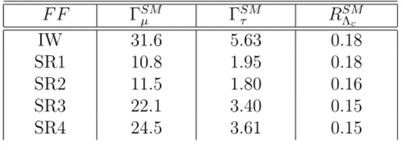
Table 2 shows the values of ΓSM_µ and ΓSM_τ , calculated by means of Eq. (54), and the ratio RSM

Λc = Γ

SM

τ /ΓSMµ , for the five different FF considered in the article. It can be seen that

the SM results of the partial widths depend strongly on the FF. In particular, as regards ΓSM_µ , the IW FF gives the best approximation of the experimental value, i. e.[59],

Table 2: ΓSM

µ , ΓSMτ (in µeV ) and the ratio RSMΛc = Γ

SM

τ /ΓSMµ , for the five different FF

considered. F F ΓSM µ ΓSMτ RSMΛc IW 31.6 5.63 0.18 SR1 10.8 1.95 0.18 SR2 11.5 1.80 0.16 SR3 22.1 3.40 0.15 SR4 24.5 3.61 0.15

Our result agrees also with the numerical value given in ref. 53. Instead, two of the SR FF differ from this value by more than one standard deviation and probably they need an overall normalization factor. However, we consider in the present article mainly ratios between dimensional quantities, which appear to be barely dependent on the FF. A first example is offered by the ratio R_ΛSM_c , listed in the last column of Table 2.

This table and Eq. (6) entail a prediction for RΛc. Indeed, averaging over the five

values yields ¯

RSM_Λc = 0.164 ± 0.006, R¯Λc = 0.205 ± 0.013 ± 0.008. (56)

Here the former ratio is only affected by the systematic error caused by the FF uncertainty, while for the latter also the statistical one (0.013) has to be accounted for. The smallness of the theoretical error confirms assumption 4). A particular attention deserves the IW FF. First of all, it allows to check immediately our formula (54) against the expression of the well-known muon decay width, as shown in Appendix B. Secondly, it yields, for R_ΛSM_c and for the other dimensionless quantities considered in our article, results that are similar to those obtained with the SR FF, although structurally different.

On the contrary, our result for RSM

Λc is considerably smaller than those given by the

other authors. Indeed, such values span from 0.26[46] to 0.38[50], being concentrated, in recent years, between 0.31 and 0.34[42, 49, 43, 52, 41, 47, 56]. Refs. 52 and 56 give more complete reviews of these results. In any case, the analysis exposed in the following sections is presumably independent of such a discrepancy, as it is based on the ratios χ and r± (Eqs. (59) and (60) respectively), which depend exclusively on the decay (2).

6

Couplings of the Various NP Interactions

6.1

Argand Diagrams for the NP Couplings

Table 3 provides the values of ΓI_τ and ΓN_τ for the S-, P - and R-interaction, calculated by Eq. (53) together with the equations analogous to (54). The parameters corresponding to the H-interaction can be deduced from the following linear combinations:

ΓI,H_τ = ΓI,S_τ − ρΓI,P

Table 3: Values of ΓI

τ and ΓNτ (in µeV ) for S, P and R-interactions and for the five

different FF F F ΓI,S τ ΓI,Pτ ΓI,Rτ ΓN,Sτ ΓN,Pτ ΓN,Rτ IW 1.28 0.26 -3.32 2.26 0.44 5.63 SR1 0.58 0.12 -0.67 1.03 0.19 1.95 SR2 0.60 0.12 -0.39 1.06 0.20 1.80 SR3 0.99 0.20 -1.21 1.75 0.34 3.40 SR4 1.05 0.22 -1.25 1.86 0.36 3.61

As regards the L-interaction, we have the re-scaling

|1 + xLeiϕ|2 = ξ, (58)

independent of the FF.

Eq. (53) yields, together with Eq. (7), a relation between x and ϕ. Taking account of the statistical and systematic errors, the allowed region consists of a circular crown in the Argand plane of the coupling gr, centered at

gc≡ (χ, 0), χ = − ΓI τ ΓN τ (59) and with radii

r± = √ ∆r± ΓN τ , ∆r± = (ΓIτ) 2_{+ (Γ} τ ±− ΓSMτ )Γ N τ ; (60)

here Γτ ± takes into account the statistical error of ξ±, Eq. (6), and the systematic one,

related to the FF. Exceptionally, the latter is absent for L-interaction, as Eq. (58) entails, independent of the FF,

gc ≡ (−1, 0), r±=

p

ξ±. (61)

The mean values and the statistical and systematic errors of the radii and the coordinates of centers of the Argand diagrams are listed in Table 4. Again, we remark the small theoretical errors of the parameters, which reflect the mild FF dependence.

6.2

Remarks

Two remarks are in order for the case of ϕ = ±π/2, where the interference between the SM amplitude and the NP one vanishes.

- Firstly, note that comparing the results of Table 2 and of Table 3 yields

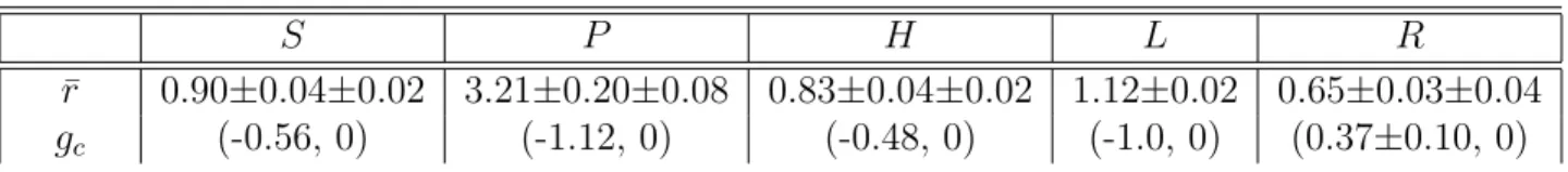
Table 4: The mean values of the radii and of the centers of the Argand diagrams for the relative couplings gr. ¯r is affected both by a statistical and a systematic error, the former

and the latter one respectively.

S P H L R

¯

r 0.90±0.04±0.02 3.21±0.20±0.08 0.83±0.04±0.02 1.12±0.02 0.65±0.03±0.04

gc (-0.56, 0) (-1.12, 0) (-0.48, 0) (-1.0, 0) (0.37±0.10, 0)

this is a consequence of the integration of Eq. (24) over the phase space, which washes out the interference term between the vector and the axial current. Therefore we have, again independent of the FF,

xR(±π/2) = xL(±π/2) = 0.50 ± 0.04. (63)

- Secondly, if one considers the possibility of decays Λb → Λcτ−ν¯`, with ` = e, µ, τ [17],

the coupling strength for ` = µ and e can be inferred just for ϕ = ±π/2.

6.3

Relative Strengths of the NP Interactions

In order to compare the strengths of the various NP interactions, we may, for example, calculate their minimal values. These occur at ϕ = 0, except for the R-interaction, for which one has to set ϕ = π. This singular behavior is due to the negative value of ΓI,R_τ (see Table 3), which induces, through Eq. (59), a real positive value of χ, and to the positivity of xmin = r − |χ|, which follows from Eqs. (59) and (60). As we shall see in a

moment, this anomaly is connected to a strong limitation on the phase ϕ. The values of xmin − once more barely FF dependent − are listed in Table 5.

6.4

Constraints from B → D

τ ¯

ν

Decays

Now we exhibit the phase limitations implied by our analysis, when combined with the analogous ones performed on the semi-leptonic B decays[15, 16, 17, 19, 60], especially the most recent ones[19].

- As regards the L-interaction, the agreement with all of the previous papers is trivial, because the NP term just re-scales the SM interaction.

- As shown before, the minimum value of x for the R-interaction occurs in correspondence of ϕ = π. This property is shared by the B → D∗τ ντ decay, whereas

the B → Dτ ντ decay indicates that the minimum occurs at ϕ = 0[17]. Therefore the

allowed region for the coupling amounts to the intersection between two circular crowns whose centers are considerably far from each other, which strongly restricts the range of values of the phase; precisely, the previous analyses provide a narrow nearby of ϕ = ±π/2[15, 17, 19]. But, as shown, in this case one has x = 0.50 ± 0.04.

- Also the H-interaction exhibits strong limitations on its phase. Indeed, we have to take into account the results of Table 4, together with those by refs. 19, that is, gc =

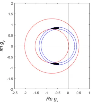
Figure 1: H-interaction: the Argand diagram for the relative coupling gr. The thinner of

the two circular crowns is inferred from our analysis, the other one from the second ref. 19, where also bounds on the phase have been established. The dark regions correspond to the range of the allowed values of gr.

(-0.76, 0.0), r = 1.03 ± 0.256_{, together with a bound on the phase[17, 19]. Then, the}

allowed region of the Argand plane amounts to two very small intervals around

ϕ = ±2.18 rad, (64)

as illustrated in Fig. 1.

- Lastly, the S + P -interaction is excluded by recent analyses[19]; similarly, the tensor interaction does not find an appreciable room[17, 19].

7

Discussion

First of all, we draw some consequences of our assumption 5) from the bounds just discussed. Secondly, we review and comment some of the previous analyses.

7.1

Analyzing the Results

- The P -interaction demands a quite large coupling (x > 2), in order to compensate the smallness of the matrix element of the corresponding operator between the initial and

final state. This appears unrealistic, also in view of the considerations by Datta et al.[47], who discard this interaction when compared with the data of the decay Bc→ τ ¯ντ.

- As a consequence, for x ≤ 1, the H-interaction (H = S − P ) behaves quite similarly to the S one, as can be seen from Tables 4 and 5. Moreover, as shown before, when combined with the previous ones, our analysis imposes strong limits on the phase, which entails a relative strength that is considerably greater than the minimal value. Indeed, in order to determine x, we set, at the left-hand side of Eq. (53), Γ` = Γτ = ξΓSMτ and fix

ϕ according to Eq. (64). The smaller root of this equation yields

x0 = 1.18 ± 0.12, x1 = 1.09 ± 0.10, x2 = 1.05 ± 0.09,

x3 = 1.09 ± 0.10, x4 = 1.09 ± 0.10, (65)

where x0 corresponds to the IW FF, the remaining xi to the SR FF. Apart from the

scarce agreement with our assumption 5), we observe that the 2HD model, included in the H-interaction, presents difficulties in explaining the anomaly[24-27], despite the fact that its coupling depends on the flavor, as required by LFUV.

- Similarly, the R-interaction − implemented by a specific model[30] − is affected, as seen, by strict limitations on the phase.

- On the contrary, as regards the L-interaction, any value of ϕ is admitted by the analyses. This entails the possibility of a small (∼ 0.12) value of the relative strength It is in qualitative agreement with a possible solution to the anomaly observed in the B → K∗`+<sub>`</sub>−_{decay[61, 57], for which a very small relative strength is required. Moreover,}

this interaction is favored in the optics of MFV[29], since it does not imply a CP violation phase out of the CKM scheme, as opposed to the cases of H- and R-interactions.

Incidentally, estimating the mass of the NP intermediate boson to be about 10 times that of the usual intermediate vector boson W , this implies that the NP coupling in the H-, R- and L-interaction is, respectively, ∼ 10, 7 and 3.5 times greater than the electroweak coupling constant.

To conclude our analysis, we remark that the L- and H-interactions recur in the most common models used to explain NP effects of the semi-leptonic decay and might be compatible with the anomaly seen in the B → K∗`+<sub>`</sub>− _{decay[22, 31, 32, 57, 62].}

According to assumption 5), the former interaction appears favored. However, as we shall see in the following subsection, alternative analyses lead to different conclusions. Therefore, measurements for discriminating among different NP interactions are suitable, as we shall exhibit in the next section.

7.2

Previous Analyses

7.2.1 Λb → Λcτ ¯ντ

Two analyses[41, 47] are quite similar to the present one, they also show Argand diagrams for the NP couplings. Shivashankara et al.[41] take into account the constraints that derive from R_D(∗) and remark that the effects produced by the P -interaction are larger than those

caused by the S-one. Datta et al.[47] fix the NP couplings so that Rratio Λc = R

ratio

3 standard deviations. Their condition is similar to ours, but less restrictive, therefore they get less severe bounds on phases and strengths of the couplings.

Dutta[43] assumes that RΛc = RD(∗) within 3 standard deviations and considers two

possible scenarios, either a mixing of L- and R-, or of H- and S + P -interactions. In the former case, he finds that only the L- or the purely vector interaction are possible. On the contrary, either the H- or the S-interaction survives the latter scenario, with more restrictions on the parameter space. This is not in contradiction with our results.

Li et al.[46] analyze the decay in the framework of the leptoquark model, taking account of the B → τ ν decay. They examine either the vector or the scalar case, finding more restrictions for the latter alternative.

7.2.2 B → D(∗)τ ¯ντ

We signal here two analyses of the B-decay, alternative to those considered above, which lead to different conclusions about the NP interaction.

S. Bhattacharya et al.[21] fit the FF to the data of the B → D(∗)_{τ ¯ν}

τ decay using only

the SM term; then they compare such FF with those available from B → D(∗)`¯ν` data,

finding a disagreement only as regards the axial current. To choose among the various NP operators, they use information-theoretic approaches and goodness-of-fit tests for cross validation, indicating the R-interaction as the best one.

Celis et al.[63] consider it difficult to explain LFUV with L- and R-interactions and perform a comprehensive analysis of the scalar contributions in b → cτ ντ transitions.

The authors examine various observables, like R_D(∗), the q2 differential distributions of

B → D(∗)_{τ ¯ν}

τ and the τ polarization in B → D∗τ ¯ντ and the Bc lifetime. They find that,

in the framework of scalar NP, the discrepancy with the SM can be explained by a mixing of H- and S + P -interaction, with a slight tension for RD∗.

8

Alternative Observables for New Physics

8.1

Previous Proposals

In order to discriminate among the possible NP interactions, various observables have been proposed for the semi-leptonic Λb decays. We recall especially the τ or Λc

polarization[42], the forward-backward asymmetry on the lepton side[42, 47] and the differential observable[41, 47] BΛc(q 2_{) =} dΓτ dq2/ dΓ` dq2, (66)

where dΓτ (`)/dq2 is the differential width of the semi-leptonic Λb decay, with the τ -

(`)-lepton in the final state.

As regards the B semi-leptonic decays, some asymmetry[38, 60] and the polarization of one of the final products[12, 14, 17, 19, 27, 64], especially its T-odd component[19], have been suggested.

Table 5: Minimal values of the relative strength x for the various interactions and for the different FF. F F xS xP xH xL xR IW 0.41±0.10 2.44±0.51 0.43±0.10 0.12±0.04 0.18±0.05 SR1 0.33±0.09 2.08±0.45 0.35±0.09 0.12±0.04 0.26±0.07 SR2 0.30±0.08 1.91±0.42 0.32±0.08 0.12±0.04 0.33±0.07 SR3 0.33±0.09 2.08±0.45 0.35±0.09 0.12±0.04 0.26±0.07 SR4 0.33±0.09 2.06±0.45 0.35±0.09 0.12±0.04 0.26±0.07

In this connection, we remark that a a T -odd observable could help to reveal a non-trivial phase ϕ, which seems to occur in the cases of H- and R-interactions.

8.2

A New Suggestion

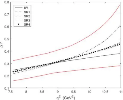
As an alternative to the observables just exposed above, we propose the following one: ∆r(q2) = BΛc(q 2₎ BSM Λc (q 2₎ − 1 = dΓτ dq2/( dΓτ dq2)SM− 1. (67)

Fig. 2 shows the behavior of this quantity in the case of the H-interaction, assuming, as found before, ϕ = ±2.18 rad and the strengths (65) for the different FF. Once more, it does not depend so dramatically on the FF.

As regards the L-interaction, one has, independent of the FF,

∆r(q2) = 0.25 ± 0.04 (68)

for any ϕ. This is equal to the distribution (67) for the R-interaction at ϕ = ±π/2.

9

Conclusions

Let us stress the most relevant points of our paper.

A) As already observed in sect. 5, the results concerning the partial widths depend rather strongly on the FF. On the contrary, the dimensionless parameters r, χ and x, as well as the observables RΛc, R

ratio

Λc and ∆r(q

2_{), exhibit, similarly to ref. 41, a mild FF}

dependence, contained within ∼ 2 − 3%. Actually, such uncertainties vanish at all if the L-interaction is assumed. Yet, our prediction on RΛc differs considerably from those by

other authors.

B) We have done some assumptions, generally shared by the other authors, furthermore we have adopted a particular criterion for choosing the type of NP interaction. We have also taken into account the analyses of the B semi-leptonic decays and the most commonly used models. On this basis, our calculations indicate that the most likely NP

Figure 2: The observable ∆r, Eq. (67), as a function of q2_{, with ϕ = ± 2.18 rad; see Eqs.}

(65) for the corresponding values of x. The upper and lower curve delimit the allowed band.

interactions are the L- and H-one. But the former interaction appears simpler and more natural.

C) Our conclusions about the NP term are in contrast with those by other authors. At this point the measurements of alternative observables, like polarization or other asymmetries, is determinant. In particular, we have proposed a differential observable which could allow to discriminate between the two NP interactions mentioned at point B).

Acknowledgments

The authors are thankful to their colleagues Fajfer et al.[12, 15] and Ivanov et al.[19] for helpful communications and suggestions.

Appendix A

Here we show that the operators

Vµ = f1γµ+ f2iσµνqν + f3qµ (A. 1)

and

Aµ= (g1γµ+ g2iσµνqν+ g3qµ)γ5, (A. 2)

when inserted between the initial and the final baryon state, can be re-written as

Vµ = [f1− (mi+ mf)f2]γµ+ f2Pµ+ f3qµ, (A. 3)

Aµ = {[g1+ (mi− mf)g2]γµ+ g2Pµ+ g3qµ}γ5, (A. 4)

thanks to the equations of motion (eom). Here

q = pi− pf, P = pi+ pf (A. 5)

and pi(f ) is the four-momentum of the initial (final) baryon.

To this end, we consider the matrix element i¯ufσµνuiqν = − 1 2u¯f(γµγν − γνγµ)ui(p ν i − p ν f). (A. 6)

By using the eom and the relationship

(γµγν + γνγµ) = 2gµν, (A. 7) we get ¯ uf(γµγν− γνγµ)uipνi = 2(miu¯fγµui− ¯ufuipiµ), (A. 8) ¯ uf(γµγν − γνγµ)uipνf = 2(¯ufuipf µ− mfu¯fγµui). (A. 9)

Inserting these two expressions into Eq. (A. 6) yields

i¯ufσµνuiqν = ¯ufuiPµ− (mi+ mf)¯ufγµui. (A. 10)

By considering the matrix element ¯ufVµui and taking account of Eq. (A. 10), we get Eq.

Appendix B

Here we verify that the formula used for the differential decay width amounts, under the suitable substitutions, to well-known expression for the muon decay, µ− → e−_ν

µν¯e.

Eqs. (45), (46) and (25) yield dΓSM ` dEf = 2mi dΓSM ` dq2 = |Vcb|2 26_π3_m i G2 2 Z E_{`</sub>+ E<sub>`}− dE`TSM. (B. 1)

Here E` and Ef are respectively the energies of the final baryon and of the charged lepton

in the Λb rest frame, with E`± given by Eqs. (47). For the sake of simplicity, we assume

the Isgur-Wise form factor; then Eq. (30) entails

TSM = 27pf · p` pi· p ζ02[ω(Ef)], ω(Ef) =

Ef

mf

, (B. 2)

with ζ0[ω(Ef)] given by Eqs. (22) and (23). Then

dΓSM ` dEf = |Vcb| 2 π3 G 2 ζ<sub>0</sub>2[ω(Ef)] Z E<sub>`</sub>+ E<sub>`</sub>− dE`[−miE`2+ A0(Ef)E`+ B0(Ef)], (B. 3) with A0(Ef) = −2miEf + 1 2M 2_{+ m}2 i, (B. 4) B0(Ef) = −miEf2+ (miM0+ 1 2M 2_)E f + 1 2(m 2 `mf − M2M0), (B. 5) M2 = m2_i + m2_f + m2_l, M0 = mi+ 1 2mf. (B. 6)

In order to recover the differential width of the muon decay, we substitute

mi → mµ, mf, m` → 0, ζ0, Vcb→ 1. (B. 7)

Therefore Eq. (B. 3) yields dΓSM_` dEf → dΓ SM µ dEe = G 2 π3mµ[− 1 3δ3(Ee) + 1 2A(Ee)δ2(Ee) − B(Ee)δ1(Ee)]. (B. 8) Here A(Ee) = 1 2(3mµ− 4Ee), B(Ee) = 1 4(2E 2 e − 3mµEe+ m2µ), (B. 9) δ1(Ee) = √ ∆ q2 , δ2(Ee) = δ1(Ee) b q2, δ3(Ee) = δ1(Ee) b2 + q2c (q2₎2 ; (B. 10)

moreover, ∆, b and c are given by Eqs. (47) to (50), taking into account the substitutions (B. 7). Substituting Eqs. (B. 9) and (B. 10) into Eq. (B. 3), we get the energy spectrum of the electron emerging from the muon decay[65]:

dΓSM_µ dEe = mµG 2 12π3 E 2 e(3mµ− 4Ee). (B. 11)

The calculation of the SM differential and decay width, Eq. (B. 3), has been performed analytically. The partial decay width has been obtained by integrating numerically the differential one between mf and Efm, according to Eqs. (52). An analogous procedure

has been employed for the contributions due to new physics. To this end, the tool Mathematica[66] has been used. The same results, exposed in Tables 2 and 3, have been obtained also by means of Matlab[67].

References

[1] S. Chatrchyan et al., CMS Coll.: Phys. Lett. B 716 (2012) 30 [2] G. Aad et al., ATLAS Coll.: Phys. Lett. B 716 (2012) 1

[3] J.P. Lees et al., BaBar Coll.: Phys. Rev. Lett. 109 (2012) 101802 [4] J.P. Lees et al., BaBar Coll.: Phys. Rev. D 88 (2013) 072012 [5] M. Huschle et al., Belle Coll.: Phys. Rev. D 92 (2015) 072014 [6] Y. Sato et al., Belle Coll.: Phys. Rev. D 94 (2016) 072007 [7] S. Hirose et al., Belle Coll.: Phys. Rev. Lett. 118 (2017) 211801 [8] R. Aaij et al., LHCb Coll.: Phys. Rev. Lett. 115 (2015) 111803 [9] R. Aaij et al., LHCb Coll.: Phys. Rev. Lett. 111 (2013) 191801 [10] R. Aaij et al., LHCb Coll.: Phys. Rev. Lett. 113 (2014) 151601 [11] J.F. Kamenik and F. Mescia: Phys. Rev. D 78 (2008) 014003 [12] S. Fajfer et al.: Phys. Rev. D 85 (2012) 094025

[13] J.A. Bailey et al., Fermilab Lattice and Milc Coll.: Phys. Rev. Lett. 109 (2012) 071802; Phys. Rev. D 92 (2015) 034506

[14] J.P. Lee: Phys. Lett. B 526 (2002) 61

[16] A. Datta et al.: Phys. Rev. D 86 (2012) 034027

[17] M. Tanaka and R. Watanabe: Phys. Rev. D 87 (2013) 034028 [18] P. Biancofiore et al.: Phys. Rev. D 87 (2013) 074010

[19] M.A. Ivanov et al.: Phys. Rev. D 94 (2016) 094028; Phys. Rev. D 95 (2017) 036021 [20] D. Choudhury et al.: Phys.Rev. D 95 (2017) 035021

[21] S. Bhattacharya et al.: Phys. Rev. D 93 (2016) 034011; Phys. Rev. D 95 (2017) 075012

[22] L. Di Luzio and M. Nardecchia: Eur. Phys. Jou. C 77 (2017) 536 [23] F.U. Bernlochner et al.: Phys. Rev. D 95 (2017) 115008

[24] L. Dhargyal: Phys. Rev. D 93 (2016) 115009 [25] J.P. Lee: Phys. Rev. D 96 (2017) 055005

[26] S. Iguro and K. Tobe: Nucl. Phys. B 925 (2017) 560

[27] C.-H. Chen and T. Nomura: Eur. Phys. Jou. C 77 (2017) 631 [28] Y. Sakaki et al.: Phys. Rev. D 88 (2013) 094012

[29] M. Freytsis et al.: Phys. Rev. D 92 (2015) 054018 [30] R. Barbieri et al.: Eur. Phys. Jou. C 77 (2017) 8 [31] A. Crivellin et al.: JHEP 1709 (2017) 040

[32] Y. Cai et al.: JHEP 1710 (2017) 047 [33] D. Buttazzo et al.: JHEP 1711 (2017) 044

[34] M. Bordone et al.: Phys. Rev. D 96 (2017) 015038

[35] X.-G. He and G. Valencia: Phys. Rev. D 87 (2013) 014014; Phys. Lett. B 779 (2018) 52

[36] W. Altmannshofer et al.: Phys. Rev. D 96 (2017) 095010 [37] A. Biswas et al.: Phys.Rev. D 97 (2018) 035019

[38] C.-H. Chen and C.-Q. Geng: Phys. Rev. D 71 (2005) 077501 [39] W. Detmold and S. Meinel: Phys. Rev. D 93 (2016) 074501 [40] T. Gutsche et al.: Phys. Rev. D 87 (2013) 074031

[41] S. Shivashankara et al.: Phys. Rev. D 91 (2015) 115003 [42] T. Gutsche et al.: Phys. Rev. D 91 (2015) 119907 [43] R. Dutta: Phys. Rev. D 93 (2016) 054003

[44] N. Habyl et al.: Int. Jou. Mod. Phys. Conf. Ser. 39 (2015) 1560112 [45] E. Di Salvo and Z.J. Ajaltouni: Mod. Phys. Lett. A 32 (2017) 1750043 [46] X.Q. Li et al.: JHEP 1702 (2017) 068

[47] A. Datta et al.: JHEP 1708 (2017) 131

[48] R. Dutta and A. Bohl: Phys. Rev. D 96 (2017) 076001 [49] W. Detmold et al.: Phys. Rev. D 92 (2015) 034503 [50] M. Pervin et al.: Phys. Rev. C 72 (2005) 035021 [51] T. Gutsche et al.: Phys. Rev. D 90 (2014) 114033

[52] R.N. Faustov and V.O. Galkin: Phys. Rev. D 94 (2016) 073008 [53] H.-W. Ke et al.: Phys. Rev. D 77 (2008) 014020

[54] R. Aaij et al., LHCb Coll.: Phys. Rev. D 96 (2017) 112005 [55] R.S.M. De Carvalho et al.: Phys. Rev. D 60 (1999) 034009 [56] K. Azizi and J.Y. Sungu: Phys. Rev. D 97 (2018) 074007 [57] D. Choudhury et al.: Phys. Rev. Lett. 119 (2017) 151801

[58] Y. Amhis et al., HFLAV coll.: Eur. Phys. Jou. C 77 (2017) 895 [59] C. Patrignani et al.: Chin. Phys. C 40 (2016) 100001

[60] M. Duraisamy and A. Datta: JHEP 1309 (2013) 059 [61] S. Glashow et al.: Phys. Rev. Lett. 114 (2015) 091801 [62] B. Bhattacharya et al.: Phys. Lett. B 742 (2015) 370 [63] A. Celis et al.: Phys. Lett. B 771 (2017) 168

[64] A.K. Alok et al.: Phys. Rev. D 95 (2017) 115038

[65] L.B. Okun: Leptons and Quarks, Elsevier Science Publishers B.V., 1982, 1984 [66] Wolfram Research, Inc., Mathematica, Version 11.3, Champaign, IL (2018)

[67] MATLAB Release 2016b, The MathWorks, Inc., Natick, Massachusetts, United States