Barriers to the adoption and optimal use of savings and health technologies

(1)

Barriers to the Adoption and Optimal Use of Savings and Health

Technologies

by

Simone Gabrielle Schaner

A.B. Economics, Princeton University (2003) Submitted to the Department of Economics in partial fulfillment of the requirements for the degree of

Doctor of Philosopy at the

MASSACHUSETTS INSTITUTE OF TECHNOLOGY June 2011 MASSACHUSETTS INSTITE OF TECHNOLOGY

JUN 10 2011

LIBRARIES

@

The author hereby grants to MIT permission to reproduce and distribute publicly paper and electronic copies of this thesis document in whole or in part in any medium now known

or hereafter created. A uthor...

...

Thnartment of Economics May 13, 2011 Certified by

...

Abhijit Banerjee

A

International Vrofessor of Economics Thesis Supervisor Certified by

Abd, I T T---- '-a-* 1 'T- '

...

Esther Duflo ion and Development Economics

Thesis Supervisor

Certified by..

...

Tavneet Suri Assistant Professor of Applied Economics, MIT Sloan School of Management

Thesis Supervisor

A ccepted by ...

Esther Duflo Abdul Latif Jameel Professor of Poverty Alleviation and Development Economics Chairman, Departmental Committee on Graduate Studies

(2)

Barriers to the Adoption and Optimal Use of Savings and Health Technologies

by

Simone Gabrielle Schaner

Submitted to the Department of Economics on May 13, 2011, in partial fulfillment of the

requirements for the degree of Doctor of Philosopy

Abstract

This thesis studies Kenyan households' use of savings accounts and malaria testing and treatment technologies.

The first chapter studies whether or not married couples use savings accounts strategically. In the absence of commitment, the availability of a "private" savings technology (a device that is only accessible by a single owner) may incite individuals to take costly strategic savings action in order to manipulate the time path of consumption. This chapter presents a model that formalizes this idea and derives several testable theoretical implications. In particular, households where husbands and wives are well matched in terms of time preference should make greater use of joint (public) accounts, less use of individual (private) accounts, and make more efficient investment choices as compared to their poorly matched peers. The model informed the design of a field experiment where married couples in rural Kenya were given the opportunity to open joint and individual bank accounts at randomly assigned interest rates. The behavior of individuals in the experiment is inconsistent with ex-ante Pareto efficiency and a variety of alternative models of intrahousehold resource allocation, but consistent with the proposed model of strategic savings. Savings misallocation due to strategic behavior may be substantial: in the experiment poorly matched couples forgo at least 64 percent more interest than well matched couples.

The second chapter studies the impact of reducing bank account transaction costs. Free ATM cards were offered to a randomly selected subset of newly opened formal bank accounts in Western Kenya. The ATM card reduced withdrawal fees by over 50 percent (from $0.78 to $0.38) and enabled account holders to make withdrawals from their accounts at any time of the day. The cards also enabled accounts to be accessed without the in-person verification of a national identity card. Targeting ATM cards to joint accounts and accounts owned by men substantially increased savings rates (by 39 percent) and average daily balances (by 16 percent) in the bank accounts. In contrast, the intervention had a negative impact when targeted to individual accounts owned by women. This gender difference appears to be driven by differences in bargaining power within the household: the positive treatment effect for men is concentrated in households where men have above median bargaining power, whereas the negative treatment effect for women is concentrated in households where women have below median bargaining power.

The final chapter (co-authored with Jessica Cohen and Pascaline Dupas) uses data from a randomized controlled trial conducted with over 2,900 households in rural Kenya to study the tradeoffs between the affordability of effective antimalarials (ACTs) and overuse. We compare a 95-percent ACT subsidy (currently under consideration by the global health community) to an alternative policy regime that explicitly acknowledges the problem of overuse by providing access to a subsidized rapid diagnostic test for malaria (RDT) in tandem with subsidized ACTs. We find that ACT access increases by 60 percent in the presence of an ACT subsidy of 80 percent of more. Under the proposed 95-percent ACT subsidy, however, only 56 percent of those buying an ACT at

(3)

the drug shop test positive for malaria. We show that targeting could be substantially increased (without compromising access) when the ACT subsidy is reduced to 80 percent but accompanied

by an RDT subsidy.

Thesis Supervisor: Abhijit Banerjee

Title: Ford International Professor of Economics Thesis Supervisor: Esther Duflo

Title: Abdul Latif Jameel Professor of Poverty Alleviation and Development Economics Thesis Supervisor: Tavneet Suri

(4)

Acknowledgments

I owe a debt of gratitude to many, and this list is sure to be incomplete. First, I thank my advisors,

Abhijit Banerjee, Esther Duflo, and Tavneet Suri, for invaluable advice and feedback at all stages of my thesis research. They have taught me much, and it has been a great pleasure working with them. Over my graduate career I have benefited from the advice and tutelage of many more MIT faculty members - Ben Olken, Rob Townsend, and Josh Angrist deserve special mention. I also thank Garance Genicot and Dean Karlan, who nurtured my interest in development economics as an undergraduate, and my colleagues at the Urban Institute (especially Pam Loprest), who inspired me to get a Ph.D. in economics.

Identification issues aside, I can confidently say that the MIT peer effect is large, positive, and

highly significant. My classmates have been great teachers, colleagues, and friends. Special thanks

go to current and past office mates Dan Keniston, Emily Breza, Cynthia Kinnan, Nick Ryan, Rick Hornbeck, and Jeremy Shapiro.

My first two chapters would not have been possible without the tireless assistance, hard work,

and commitment of many employees of Family Bank. I am particularly indebted to Victor Keriri Mwangi, Steve Mararo, and Michael Aswani Were. I also thank Noreen Makana for her superb field management, Moses Baraza for his expert advice, and the IPA enumerators for their excellent assistance with the data collection. Andrey Vakhovskiy provided much appreciated support and advice during field activities.

It has been an utter pleasure working with Jessica Cohen and Pascaline Dupas on the third chapter of this thesis. They have been wonderful collaborators and have taught me a great deal about both field work and economics.

I gratefully acknowledge the financial support of the Russell Sage Foundation, the George and

Obie Shultz Fund, and MIT's Jameel Poverty Action Lab (Chapters 1 and 2), the Clinton Foundation Health Access Initiative and Novartis Pharmaceuticals (Chapter 3), and the and the National Science Foundation's Graduate Research Fellowship.

Most of all, I thank my wonderful parents, Peter and Nancy Schaner - their unwavering love, support, and belief in me has sustained me not just through graduate school, but throughout my life.

(5)

1.C

Alternative Explanations . . . . Conclusion . . . . Appendix: Proofs . . . . Appendix: Extra Statements Sample... Appendix: Tables and Figures . . . .

. . . . 4 9

. . . . 5 0 . . . . 5 2 . . . . 5 8

... . . . . . . . . 59

2 Cost and Convenience: The Impact of ATM Card Provision Account Use in Kenya 2.1 Introduction . . . . 2.2 Theoretical Framework.. . . . . . . . .. 2.3 Experimental Design and Data . . . . 2.3.1 Experimental Context . . . .. 2.3.2 Experimental Design . . . . 2.3.2.1 Targeted Population . . . . 2.3.2.2 Interest Rates . . . . 2.3.2.3 ATM Cards . . . . 2.3.3 D ata . . . . 2.3.4 Sample Characteristics and Randomization Verification 2.4 R esults . . . . 2.4.1 Summary of Account Use . . . . 2.4.2 Impact of ATM Card Provision . . . . 2.4.3 Bargaining Power and ATM Card Treatment Effects . . . 2.5 C onclusion . . . . 2.A Appendix: Additional Time Preference Analysis . . . . 2.A.1 Survey Questions on Rates of Time Preference . . . . 2.A.2 Time Inconsistency and ATM Card Treatment Effects 2.B Appendix: Tables and Figures . . . . on Formal Savings 81 . . . . 8 1 . . . . 83 . . . . 86 .. . . . .. 86 . . . . 86 . . . . 86 . . . . 87 . . . . 88 . . . . 88 . . . . 89 . . . . 9 1 . . . . 9 1 . . . . 93 . . . . 98 . . . 10 1 . . . 103 . . . 103 . . . .. 104 . . . 105

3 Price Subsidies, Diagnostic Tests, and Targeting of Malaria Treatment: Evidence from a Randomized Controlled Trial* 123 3.1 Introduction . . . 123

3.2 Background .. .. ... . ... . ... . . . .. . . . .. .. .. 128

3.2.1 Background on M alaria . . . 128

3.2.2 The Affordable Medicines Facility for Malaria (AMFm) . . . 129 *This chapter is co-authored with Jessica Cohen and Pascaline Dupas.

1.4.2

1.4.3

(7)

3.2.3 Health Providers and Health Treatment Seeking in Rural Kenya 3.3 Model . . ... ... .. ... . .. ... . 3.3.1 3.3.2 3.3.3 3.4 Study M odel Setup . . . .

Impact of an ACT Subsidy at the Drug Shop . Impact of Adding an RDT Subsidy at the Drug Design and Data . . . .

Shop

3.4.1 Experimental Design . . . .

3.4.2 D ata . . . .

3.4.3 Characteristics of Study Sample . . . .

3.5 R esults . . . .

3.5.1 Predicting Malaria Positivity . . . .

3.5.2 Status Quo Treatment-Seeking Behavior . . . .

3.5.3 The Impact of Subsidies on Treatment Seeking Behavior 3.5.4 Within-Subsidy Price Variation, ACT Access, and ACT

3.6 Cost Effectiveness . . . . 3.6.1 Methodology . . . .

3.6.2 R esults . . . .

3.7 C onclusion . . . .

3 A Appendix: Predicted Positivity and Regression Bias . . . .

Targeting

3.B Appendix: Tables and Figures .

129 131 132 132 134 135 135 137 138 139 139 140 141 146 149 149 150 152 153 156 176 Bibliography . . . . . . . .

(8)

(9)

Chapter 1 Intrahousehold Preference Heterogeneity,

Commitment, and Strategic Savings:

Theory and Evidence from Kenya

1.1 Introduction

Informal and semi-formal savings devices abound in the developing world, even though they are generally characterized by high costs, illiquidity, and substantial risk (Rutherford 1999; Rutherford 2000).1 Moreover, households often use a variety of such arrangements (Collins, Morduch, Ruther-ford, and Ruthven 2009), even though storing savings at home should be essentially costless in the absence of complications. As such, the popularity of these devices presents a puzzle - what constraints make these costly practices attractive? Recent research reveals three central themes: the need to protect savings from oneself (as in Ashraf, Karlan, and Yin 2006), the need to pro-tect savings from appropriation by members of the community (as in Baland, Guirkinger, and Mali

2007), and the need to protect savings from other members of the household, especially one's spouse

(as in Anderson and Baland 2002). This final theme presents a particular challenge to traditional economic representations of the household - since members share a unified budget constraint and interact repeatedly, they should be able to contract with one another in a Pareto efficient manner, even when they have different preferences (Browning and Chiappori 1998). While a growing number of papers have documented evidence of households behaving in ways incompatible with Pareto

effi-'A stark example is that of deposit collectors. Deposit collectors regularly visit their clients to take savings deposits. They are free to do what they wish with the deposits while they store them, and they often charge fees for the service. Steel and Aryeetey (1994) document that in Ghana, these fees amount to an annual return of negative 54 percent. Another popular informal device is rotating savings and credit associations (ROSCAs). ROSCAs consist of a group of individuals who meet at predetermined intervals (e.g. weekly, monthly) to put a fixed amount of money into a common pot. At each meeting, a different member of the group receives the pot. ROSCAs are by nature illiquid and often quite risky, as group members can defect before the ROSCA cycle is completed.

(10)

ciency (see, for example, Ashraf 2009; de Mel, McKenzie, and Woodruff 2009; Duflo and Udry 2004; Robinson 2008; Udry 1996), the underlying causes of these inefficiencies remain poorly understood. To make progress on this front, this paper abstracts from all but one potential driver of inefficient household savings behavior: intrahousehold heterogeneity in rates of time preference, coupled with an inability to commit to binding contracts. The idea here is that when one household member is very impatient, he may be tempted to spend any readily accessible savings, even if he promises not to do so. In this case, other household members may resort to saving in a "private" device (such as an individual bank account) that cannot be accessed by the less patient individual, even if using this device is very costly (because it offers a negative rate of return, for instance). To formally study this mechanism, we develop a model of a two person household where individuals have access to two classes of savings devices: a private savings device and a "public" savings device (such as a joint bank account), which can be accessed by any member of the household. These savings devices may also differ in terms of rates of return and transaction costs.

We show that when discount factors within the household differ, implementing the ex-ante Pareto efficient consumption allocation requires the ability to commit to binding intertemporal contracts. When individuals cannot commit, they may be tempted to make strategic use of private accounts in order to manipulate the time path of consumption. The model underscores that both agents in the household may privately benefit from saving strategically. The more patient agent would like to push additional consumption into the future, while the less patient agent would like to push additional consumption into the present - in both cases it may be possible to achieve these goals through the use of private accounts. Moreover, the model illustrates that impatient individuals may be willing to take costly action to deny the household higher return savings devices. In this context households may make intensive use of lower return, higher transaction cost savings devices, even when more attractive (from a rate of return perspective) alternatives are readily available.

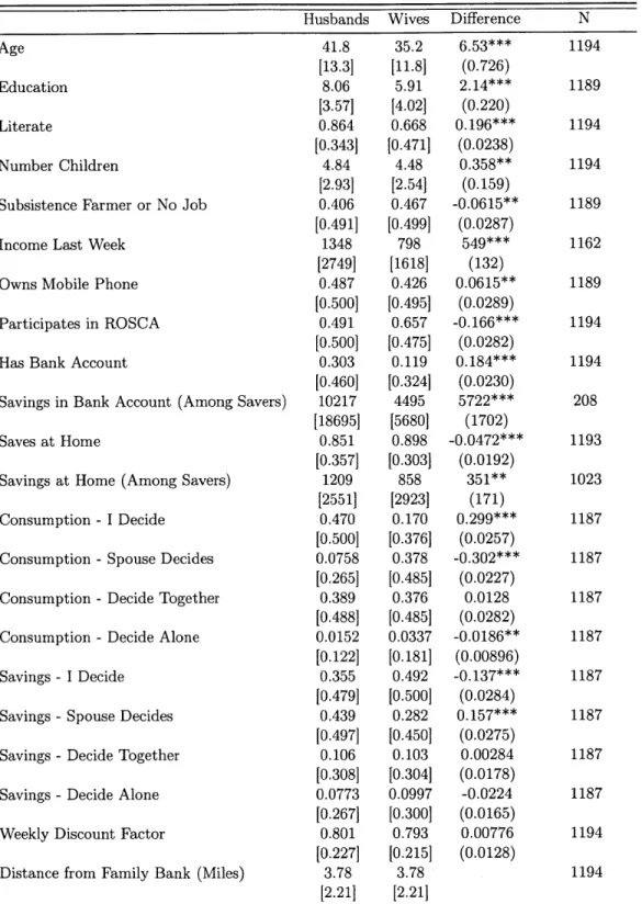
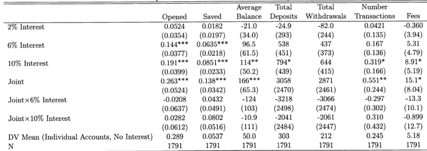
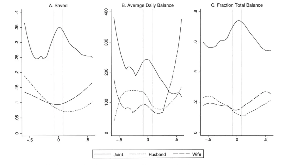
This model informed the design of a field experiment, which was conducted in Western Kenya in the Summer of 2009. We gave 597 married couples the opportunity to open three savings accounts at randomly assigned interest rates: an individual account for the husband, an individual account for the wife, and a joint account. We also asked each respondent in the experiment a battery of questions designed to elicit discount factors, which are used to calculate measures of intrahousehold discount factor heterogeneity. By applying our theoretical results to the context of the experiment, we are able to derive a series of testable predictions of the private savings model. A central theoretical result is that couples who are well matched in terms of discount factors invest their resources efficiently, while poorly matched couples savings decisions are distorted by strategic action. A key feature of the experimental design is that it created random variation in relative rates of return, even conditional on an account's own interest rate. Our theory has sharp predictions regarding patterns of account use by match quality and the shape of well matched couples' response to relative rates of return, both of which we test in the data.

(11)

terms of rates of time preference make more intensive use of joint accounts, less intensive use of individual accounts, and respond to relative rates of return in a manner consistent with investment efficiency. In contrast, poorly matched couples are completely insensitive to relative rates of return. These differences in behavior have financial consequences for poorly matched couples - interest rate losses on this group's newly opened bank account deposits were 64 percent larger than those of their well matched peers. The empirical results also suggest that transaction costs play a very important role in determining bank account choice and use in our sample.

Overall, our results are consistent with our theory of strategic savings behavior and inconsistent with ex-ante Pareto efficient bargaining. The results do not appear to be driven by a correlation between discount factor heterogeneity and other characteristics of couples. Moreover, the patterns in the data are not consistent with other theories of household saving such as mental accounting or rules of thumb.

We also investigate an alternative theory that could generate the patterns we observe in the data: hidden savings. While our model presumes complete information, agents may use private accounts to systematically hide resources from other household members (as in Anderson and Baland 2002). We make use of a randomized information treatment that we implemented as part of the field experiment, as well as spousal cross reports of income and savings device use to examine the role that hidden information plays in household savings decisions. We find evidence that households with poor information flows are more likely to choose individual accounts, less likely to choose joint accounts, and more likely to reduce savings in response to the information treatment. However, these concerns are unrelated to our initial findings regarding preference heterogeneity; well matched couples have no better information flows than poorly matched couples, and the empirical results are unchanged when accounting for intrahousehold information sharing.

The remainder of the paper is structured as follows: Section 1.2 presents our model of strategic savings behavior, Section 1.3 outlines the experimental design and derives testable implications of the theory, Section 1.4 presents main results, Section 1.5 extends the analysis to account for hidden information, Section 1.6 discusses alternative explanations, and Section 1.7 concludes.

1.2 A Model of Strategic Savings

We are interested in understanding how heterogeneity in discount factors impacts individuals' in-centives to engage in costly savings behavior. To do so, we develop a strategic model of a household consisting of two agents with potentially differing discount factors, who must decide how much to consume and how much to save in a portfolio of public and private savings devices. In this section we set up the model and characterize the ex-ante Pareto efficient savings allocation. We then show that when discount factors differ, individuals will have incentives to deviate from this allocation.

Given this observation, we then characterize the equilibrium of the strategic model and close the section by deriving comparative statics with respect to discount factor heterogeneity and interest

(12)

rates. Then in Section 1.3, we feed these results through the experimental design to derive testable predictions that can be taken to the data.

1.2.1 Model Setup

1.2.1.1 General Economic Environment

The household consists of a husband (M) and a wife (F). They live in a two period world with one personal consumption good, c. Individuals have deterministic income streams

{yM,

yf

}

and must decide whether or not to save any of their income for the second period. Though individuals can save for the future, there is no borrowing in this economy.2 Agents have perfect information regarding own and spousal income streams, preferences, savings strategies, and rates of return earned on savings.

1.2.1.2 Savings Technologies

Households have access to three different savings technologies:

" A public/joint bank account, which yields rate of return Rj > 1

* A private/individual husband's bank account, which yields rate of return RM > 1 * A private/individual wife's bank account, which yields rate of return RF > 1

What makes the "public" account public is that any member of the household can deposit and withdraw funds. In contrast, "private" accounts can only be accessed by their owner (though balances are known to all members of the household).

Financial markets in developing countries are often characterized by very high transaction costs (Karlan and Morduch 2010). To capture this, we add two types of costs to the model. First, while it is free to make deposits into all accounts, withdrawals incur a fee, w > 0. Second, accounts have

time and travel costs associated with them, which we refer to as "banking costs". The idea here is that the bank is located in town, while most individuals live outside of town. If individual i is going to town for some other reason in period t, the cost of travelling to the bank is low. However, if the individual must travel to town specifically to go to the bank, the cost is high. An important advantage of a joint account is that the couple can always send the spouse with the lowest travel cost to the bank. To capture this intuition with minimal complexity, we assume that travel costs are nonstochastic, but that the cost of travel for an individual account, b, i E {M, F}, exceeds the cost of travel for a joint account, b (i.e. b' ; b>).

2

A perfect savings and credit market without transaction costs would eliminate all scope for strategic behavior. However, our model would generalize to an environment with an imperfect credit market - this would just put constraints on some types of strategic behavior.

(13)

1.2.1.3 Preferences

Both members of the household i E {M, F} have CRRA preferences over the personal consumption good c' (we note that the results would be unchanged if we generalized preferences to be a CES aggregate of a personal consumption good and a public, nonrival consumption good):

U =Et E _-rT 3 iT-t I

1-0-Without loss of generality, we will assume that the wife is more patient than the husband (6_F 6 M) for the rest of the theoretical discussion.

The agents in the model act in self interested ways whenever possible. When an individual has proprietary access to a resource, we assume that he can make a unilateral decision regarding that resource - as a result, he will take the decision that maximizes his own utility without regard for spousal welfare. We refer to these choices as private decisions. In the context of the model, saving in individual accounts is a private decision, as resources stored in these accounts cannot be accessed without the consent of the owner.

However, some decisions in the household need to be made collectively (we refer to these as public decisions). If both members of the household can freely access a resource, then it cannot be distributed unless both spouses agree on the allocation. In order to reach a consensus, we assume that spouses bargain cooperatively with one another. We assume that the husband's bargaining power can be represented by p E (0, 1) and is a function of a variety of time invariant distributions

factors (as in Browning and Chiappori 1998).3

Savings allocated to the joint account is a public decision. This is because either spouse can access the joint account at any time; in order for funds to be deposited and remain in the account, the deposit must be determined by consensus. Similarly, the distribution of consumption between husband and wife is a public decision. In other words, we assume that the majority of consumption is akin to food eaten at home - since any household member can put more food on his or her plate, the final allocation must be determined by collective agreement. Note that this holds regardless of the source of the resources used to finance consumption (current income vs. joint saving vs. individual saving). Even when consumption is financed out of private savings, the act of transforming financial resources into the consumable good makes the resources appropriable by both spouses and therefore subject to collective bargaining.

3

One potential issue with our model is the assumption that distribution factors do not change over time. Indeed, the observation that distribution factors can shift unexpectedly has inspired a large body of empirical work (e.g. Angrist 2002; Bobonis 2009; Chiappori, Fortin, and Lacroix 2002; Duflo 2003; Lafortune 2010; Lundberg, Pollak, and Wales 1997). We could easily expand our framework to accommodate unexpected innovations in bargaining weights. A bigger issue is if the act of allocating savings to individual or joint accounts alters the bargaining weight (presumably by shifting outside options). We discuss whether the availability of such deviations could be driving our empirical results in Section 1.6.

(14)

This assumption is important, as it eliminates any scope for private accounts to be used to increase individual shares of aggregate per-period consumption. In practice, not all consumption choices are public decisions. However, while some consumption goods are undoubtedly best thought of as private (many "vice" goods such as alcohol and cigarettes have this property), these goods account for a small share of total expenditures of poor households in developing countries, particu-larly when compared to general food expenditures, which make up around two-thirds of all spending (Banerjee and Duflo 2007). In this context, private consumption concerns may be inframarginal to the savings motive and therefore ignorable from a modeling perspective. Moreover, ruling out private consumption motives allows us to focus on strategic action driven by differences in rates of time preference, which is the primary goal of our model. That said, private consumption deviations may well be important determinants of savings behavior, so we discuss whether such concerns could be generating our results in Section 1.6.

1.2.1.4 Timing and Strategic Actions

Within a given period, the model proceeds as follows:

1. Incomes (yM, yf) and returns from any previous period's savings are realized.

2. The husband and the wife simultaneously make private savings decisions. Denote private savings by individual i E {M, F} at time t as s'. An individual cannot save more than yt + Ris_1 - b in any period (resources he or she has proprietary access to, less the cost of

going to the bank).

3. The husband and wife observe total resources available, as well as resources saved privately,

and jointly decide how much to consume (ct). Any additional savings is placed in the joint account - denote this "household" saving as saf. The spouses also decide how to apportion consumption between husband and wife subject to ct

+

cf = ct.

4. Consumption takes place and the period ends.

1.2.1.5 Solution Concept

We solve for subgame perfect Nash equilibria of the private savings game. The strategy set for spouse i at time t is SJ = [0, y' + Ris- 1 - b']. The strategy set for the couple at time t is given by

S = - [0, Y (s') - bj], where Y (si) denotes period t resources net of private savings. A strategy for actor a E {J, M, F} is given by a probability distribution o over St.

In some cases, the private savings game will have multiple equilibria. To refine the set of equilibria that we need to consider, we make the following assumptions:

(15)

A2. If there exists more than one Nash equilibrium of a given type (pure/mixed), but one

rium Pareto dominates the others, then the couple will always choose the dominant equilib-rium.

When there are no transaction costs and more than one account bears the highest rate of return, there will be some cases in which a continuum of pure strategy equilibria exists, with each involving saving the same aggregate amount in different accounts. This result is not very robust - as we will see later on, as long as there is an arbitrarily small transaction cost associated with each account, at most one account will used in any implemented pure strategy Nash equilibrium (this is a result of imposing Assumption A2). To eliminate this knife edge multiple account case, we make the following assumption:

A3. There is always some (potentially arbitrarily small) transaction cost associated with banking:

either w > 0 or b > 0 Va E {J, M, F}.

1.2.2 Efficient Bargaining

Before studying the strategic solution, we establish an efficient benchmark by which to measure the behavior of households in our model. Since this is a multiperiod setting, we adopt the standard of

ex-ante Pareto efficiency. Any ex-ante Pareto efficient allocation can be captured by writing the optimization problem of a social planner who puts weight q on the husband's utility and weight

(1 - q) on the wife's utility. By varying 77 over [0, 1], we trace out the Pareto frontier. Here we set q equal to y (the husband's bargaining power in the collective allocation problem) - this solves for the allocation that would result if the husband and wife could write intertemporally binding contracts with one another. Then the planner's problem (or the "efficient bargaining" problem) is:

T=2 1-a T=2 F) 1-Or

max y =+ E (1 - p)M/I

o(

6_1 (cY

)

(EB)

(ct, ct, st, st, st It1 t=1 t=1

subject to

Yt + yt + E max

{

asi - w - , 0} ct cF (s > 0) (s, + b")

aE{J,M,F} aE{J,M,F}

s > 0 Va E {J, M, F}

where 1 (.) is the indicator function. Due to nonzero transaction costs, this problem is not convex. However, we can imagine the planner solving for the optimal savings allocation conditional on paying each relevant combination of transaction costs, and then selecting the plan that generates the highest utility. Since each conditional problem is convex, first order conditions will be necessary for an interior optimum. Taking first order conditions with respect to ct' and cf we see that

M (ca 1-- p( t-1

(16)

so when 6F > SM, the ex-ante Pareto efficient sharing rule necessitates that for a given ct = c M +CF

$

increase over time.4 We can use equation 1.1 to solve for the ex-ante Pareto efficient consumption Ct

sharing rule in each period:

cM = ptct and c= (1 - pt) ct where pt =

(poA1t ) ((1 - o F) c1)

Note that pt monotonically increases with p, the husband's bargaining power. When 6M < SF,

p1 > P2. In contrast, when SM = SF, pt is time invariant and equal to (it)

(t) 1+(1-A)-!

1.2.3 Incentives to Deviate from the Efficient Allocation

It may be difficult to enforce the ex-ante efficient allocation when pt evolves over time. In fact, when discount factors differ, there are incentives to deviate at both the private savings and collective bargaining stages of the game. First we show that individuals could make themselves better off by deviating from the efficient savings path. When so > 0, first order conditions from the efficient bargaining problem require that

(c)6

= SiRa (ci) 4. But when SM < SF, the wife's marginal

utility of an e increase in s? is

- (c F) (1 - P1) + SFRa (cF) - (1 - P2) ] > 0

and the husband's marginal utility of an e decrease in sa is

[(c) pi - SMRa (c2M)- P2 6 > 0

where both inequalities use pi > P2. In contrast, if 6M SF then pi = P2 and there are no individual incentives to deviate. A linear consumption sharing rule is essential for this result. If the sharing rule also depended on the level of consumption, there could be incentives to deviate in the absence of discount factor heterogeneity. We purposefully abstract away from this complication in order to focus on discount factors. However, it is important to note that assuming a linear sharing rule puts strong restrictions on individual utility functions: the per-period sharing rule will be linear if and only if puM

(ct')

+ (1 - p)UF (cF) is homothetic (indeed, we could easily rewrite our model with

more general utility functions under this assumption).5 4

This observation reflects broader issues associated with aggregating individual preferences with differing discount factors. In particular, aggregated preferences will be time inconsistent as long as positive weight is placed on at least two agents with og 4 og (Jackson and Yariv 2010). In our context, it is straightforward to show that when 6F > 6M

the effective discount factor governing the ex-ante efficient allocation asymptotes to 6F as T -+ oo. Other studies that address this aggregation problem include Feldstein (1964), Marglin (1963), Caplin and Leahy (2004), Gollier and Zeckhauser (2005), Weitzman (2001), and Zuber (2010).

5

This highlights an important point: in practice intrahousehold heterogeneity in discount factors may be correlated with heterogeneity in utility functions. As such, we will not be able to rule out that some part of the patterns we

(17)

Second, the couple may have difficulty enforcing the time varying consumption sharing rule. Imagine the spouses collectively decide upon a consumption path at t = 1. Then if they were given

the opportunity to reoptimize at time r > 1, they would choose to do so whenever 6M

#

6F, and

would reallocate a larger share of time r consumption to the less patient spouse such that pr = pi.1

Since only the less patient spouse stands to benefit from this reallocation, there may be some natural barriers to renegotiation (Ligon 2002); however, in the long run it seems implausible that households would be able to enforce allocations where one member gets an ever shrinking share of aggregate consumption. Indeed, the results in Duflo and Udry (2004), Mazzocco (2007), and Robinson (2008) all suggest that couples cannot commit intertemporally.

We therefore assume that all agents "live in the moment", in that if reoptimization is attractive in period t, they will reoptimize. Then the sharing rule will be governed by p = pi. This assumption

also implies that if an individual can make himself better off by deviating from the allocation that he would collectively choose with his spouse, he will do so. To see if this has bite, we solve (EB) for the optimal savings path imposing a time invariant, linear sharing rule. Denote cm (ct) = pct and

cF (ct) = (1 - p) ct. Then if the couple were to collectively choose s' > 0, the following equality would be satisfied for individual i

(C) = Ra6i (c')~O + Ra (1 - ci' (c2)) (6_i - 6i) (c ) (1.2)

Note that when 6F > 6M, the remainder term on the right hand side is negative for the wife and positive for the husband, which implies that (cf) - < Ra6F (cF' and (cM)-' > Ra3M (c2 ') In this case, if individuals do not take strategic action and the couple saves, the collective outcome will leave the wife feeling savings constrained and the husband feeling borrowing constrained - both would like to alter the time path of consumption if possible. It therefore seems likely that households with discount factor heterogeneity will exhibit strategic behavior. The next subsection characterizes this behavior and derives comparative statics with respect to preference heterogeneity and interest rates.

observe in the data are driven by more general preference heterogeneity. Section 1.6 discusses whether it seems likely that other forms of preference heterogeneity are driving our results.₆

This temptation to reoptimize reflects the fact that when discount factors differ, the household has time incon-sistent collective preferences (Jackson and Yariv 2010). This type of temptation problem is similar to the internal temptation problems studied by a large literature where either time inconsistent preferences or differential prefer-ences between different "selves" lead to distorted consumption and savings behavior (examples include Banerjee and Mullainathan 2010, Fudenberg and Levine 2006, Gul and Pesendorfer 2004, Harris and Laibson 2001, Laibson 1997, and O'Donoghue and Rabin 1999). We also note that heterogeneity in discount factors is not a necessary condition for a time inconsistent household: Hertzberg (2010) proposes a non-cooperative model of the household where two agents with identical exponential discount factors behave like a single time inconsistent agent.

(18)

1.2.4 The Strategic Solution

1.2.4.1 Incorporating the Sharing Rule

It is convenient to use the sharing rule to rewrite individual utility functions so that they are defined over aggregate per-period consumption ct:

UM -T=2 1-O

1 - =Et1z~ /M~tr]

F)l

'T=2

1 _a '

0jt = UtF _ Et

(f-

o c',

(1 - p), 1 -0,

Since the couple bargains cooperatively over joint savings, it will choose a Pareto efficient alloca-tion (subject to the time invariant p). This choice can be represented by the maximizaalloca-tion of a "household" utility function

H _p tM 1-P t -Et T= rC

QO )o _rUt 1-F

where Qt = pp1- -1+ (1 - p) (1 - p)- 6t. Note that

Q1 tip 1--M + (1 - A) (1 - P)1-' JF

-- = = = OM + (I - p) 6 F

The "household" discount factor, Q, is just a weighted average of individual discount factors, where the weights are given by each individual's share of aggregate consumption (also recall that p is just a rescaling of the bargaining weight, I).

1.2.4.2 The Collective Allocation Problem

We solve the model by working backwards. In the second (final) period, all parties would like to maximize consumption. Therefore agents optimally set s* s** = 0. Then the collective t = 1 saving problem is given by:

)1-0-S- aE{J,M,F} (s > 0) (S b)

arg max J 11 +

(Y1 ZEJ,,}1 --

~

> )mx{ae-w-bo)'

)1--y2

+

aE{JMF}1 (Sa > 0) max ( Ra- -U 0

Q (

~

1 - or

subject to sf > 0

where sj and sf are taken as given. Again, this problem is not convex due to transaction costs. As before, we can examine the convex subproblem by assuming that joint banking and withdrawal

(19)

costs are paid, solve for the optimal s, conditional on the costs being paid, and compare the utility of this allocation to the utility of setting sJ = 0. Then if the couple saves in the joint account, the

following household Euler condition holds:

c = QRjc2 (1.3)

1.2.4.3 Characterization of Optimal Strategies

Both individuals know the cooperative outcome given any private savings allocation s=

[sf,

si']' and endowment y = [y1, y2]'. Since we do not focus on changes in the endowment, we refer to the couple's optimal joint savings choice given a private savings allocation si as sJ (si).7 Before characterizing individual strategic behavior, it is useful to consider how each spouse can use his or her private account to manipulate consumption streams. The wife's goal is to increase consumption in the second period. She can achieve this by "oversaving" in her individual account - as long as she has sufficiently large yr, this will be a viable strategy even when her individual account is dominated (in terms of rate of return) by the joint and/or husband's account.

In contrast, the husband's goal is to increase consumption in the first period. Here, his optimal strategy will depend on the context. Suppose that in the absence of strategic behavior, the couple would collectively choose to save in his account because he has access to the best interest rate. In order to increase first period consumption he could either save less than the desired collective amount in his account, even to the point of refusing to save at all. Even when his account is dominated by the joint and/or wife's account, he may still be able to manipulate consumption streams in his favor. For example, suppose the couple would collectively choose to save in the joint account if he took no action. Then the husband could rush to the bank and preemptively save "just enough" in his account to prevent the couple from travelling to the bank again to save jointly. If this "just enough" amount results in increased first period consumption, a sufficiently impatient husband will find this deviation profitable. Note that in this case, the presence of transaction costs is essential - in their absence, this type of deviation would always result in decreased consumption in both periods. This is an important insight, particularly given our focus on developing countries: transaction costs greatly expand the scope of private savings deviations available to the less patient spouse.

We begin our characterization of optimal strategies by showing that at most one bank account will be in use in any implemented pure strategy Nash equilibrium. This will give us a very simple way to determine which households will save privately and which will not. First, we establish the following lemma:

Lemma 1 Let si = [M, sF]' be a pure strategy private savings allocation. If s' is part of a pure

strategy Nash equilibrium and either sm > 0 or s F > 0, then s'

(si)

= 0.

7

(20)

Proof. See Appendix A.

m

This lemma highlights that it is never optimal to save individually such that the couple travels back to the bank at the collective allocation stage. With this result in hand, we are prepared to show the following:

Proposition 1 No couple will choose a pure strategy Nash equilibrium to the private savings game

where more than one account is in use. Moreover, when RMSM :A RF0F, no such pure strategy equilibrium exists.

Proof. See Appendix A. *

Given this result, it is straightforward to determine which households will save privately. For each individual i, we need only check if he or she would find a pure strategy private savings choice profitable when sl = 0. If neither member does, Proposition 1 and Assumption Al imply that households default to s = sf = 0. If one or both members strictly prefer to save privately

assuming their spouse does not, then any Nash equilibrium must involve the use of individual accounts with positive probability. If a pure strategy Nash equilibrium can be constructed where just one spouse saves, the household will choose this over any mixed strategy by Assumption Al. If such an equilibrium cannot be constructed, both individuals in the household will randomize over private savings choices.

1.2.4.4 Preference Heterogeneity and Account Choice

We are now prepared to analyze how heterogeneity in rates of time preference impacts the efficiency of household investment choices. As a baseline, we show that perfectly matched households always

invest their savings efficiently:

Proposition 2 If

oM

= 6

F, then a solution to the ex-ante Pareto Efficient planning problem (EB) will always be chosen by the household in the private savings game.

m

To explore how preference heterogeneity impacts savings behavior, we fix incomes, the average household discount factor (Q), banking costs (ba), and interest rates. This lets us consider a subset of households who would all choose the same allocation in the absence of individual strategic behavior, and study how the chosen allocation changes with preference heterogeneity. The benevolent planner would also choose the same savings allocation for all these households if he were restricted to the time invariant consumption rule given by p. This allocation also corresponds to the outcome of the private savings game when 5M = SF = Q (Proposition 2). This concordance is a useful result of

choosing utility functions that result in a linear consumption sharing rule, and provides a natural benchmark for efficient behavior.8

8

However, note that these households would not all choose the same allocation if they could implement time varying consumption rules. This is easily seen by comparing the solution to (EB) for a household where 6m = 6F = Q

(21)

In order to derive comparative statics with respect to discount factor heterogeneity and account use, we need a way to index couples according to match quality. To do so, we define Y> 1 such that 3

m (-y) = and 5F (Y; P) =

(^(-P).

When -y = 1, 6

M = 6F = Q - a couple is perfectly matched. By varying -y and p conditional on Q, 8F - 5M can be made arbitrarily large (note that

6

F - 6M _i-p , which is strictly increasing in -y when -y 2 1), all while ensuring that 6M E (0, Q] and 6F E

To move forward, we need to put a bit more structure on the types of private savings choices that might be profitable for an individual. To do so, take all feasible private savings choices (the set

Si), discard choices that lead to a strictly Pareto dominated consumption allocation (as compared

to s' = 0) and assign the remaining choices to two sets, depending on how the choices change the

time path of consumption relative to the "household alternative", which prevails when s = 0:

Definition 1 Given s7', a temporally advantaged private savings choice for individual i is any

sc C S' that results in increased consumption in the first period when i = M or the second period when i = F, relative to the household alternative.

Definition 2 Given si, a temporally disadvantaged private savings choice for individual i is

any s, E S' that results in increased consumption in the second period when i = M or the first period when i = F, relative to the household alternative.

Note that temporally advantaged choices favor an individual's relatively preferred period (t = 2 for the wife and t = 1 for the husband). In contrast, temporally disadvantaged choices favor the opposite of the relatively preferred period. Denote individual i's set of temporally advantaged private savings choices given s-i as A' (sji) and the analogous set of temporally disadvantaged private savings choices as D' (si). When it does not cause confusion, we drop the dependence on sj' and simply refer to A' and D'. When

s'

> 0 results in the same consumption allocation as s' = 0, we assign A' to both A' and D'. Given this setup, we are now prepared to characterize how

the profitability of private savings changes with preference heterogeneity.

To do this, we establish "preference heterogeneity thresholds" for private savings. Specifically, we show that when temporally advantaged deviations are available, there exists a level of preference heterogeneity (indexed by -y) above which couples will always save privately. We also show that there exists a separate threshold for temporally disadvantaged deviations below which couples will always save privately. The following proposition formalizes this result:

Proposition 3 Fix Q, y, ba, and interest rates. Then the following preference heterogeneity

thresh-olds for private savings obtain:

to a household where 6m = 0 and 6F - . The household with greater preference heterogeneity will save more, all

(22)

1. Suppose AF (0) is nonempty. Then 3 p*

E

[0,1) s.t. V p

E

(p*,1) 7 ,y(p)

c

[1,oo) s.t.

all households with sharing rule p and -y > *

(p)

will exhibit private savings in any Nash equilibrium.

2. Suppose Am (0) is nonempty. Then E * E [1, oc) s.t. all households with - > -y* will exhibit private savings in any Nash equilibrium.

3. Suppose DF (0) is nonempty. Then Vp

E

(0,1) -y* (p) ; 1 s.t. all households with Y <

-y* (p) will exhibit private savings in any Nash equilibrium. It may be that

yp (p)*

= 1, in

which case no element of DF (0) will ever be profitable for the wife.

4.

Suppose DM (0) is nonempty. Then 3 -y* > 1 s.t. all households with -Y < -y* will exhibit private savings in any Nash equilibrium. It may be that -y* = 1, in which case no element of DM (0) will ever be profitable for the husband.

m

The first two thresholds apply to temporally advantaged choices. A key insight of this proposition is that no matter how wasteful a temporally advantaged private savings choice may be, we can always find a preference heterogeneity threshold beyond which an agent will find this choice profitable.

This is intuitive: as 6

M -+ 0 (OF -+ oc), the agent only cares about the first (second) period.

Since temporally advantaged choices favor this relatively preferred period by definition, in the limit agents will prefer them to si = 0 even when these choices incur higher transaction costs and/or

require the use of substantially lower interest rates. At the same time, it is important to note that private savings choices need not be inefficient - this will depend on the parameter values under consideration.

The final two thresholds apply to temporally disadvantaged choices. Here, the sign of the inequalities are reversed: since these choices favor the opposite of the agent's preferred period, they become less attractive as preference heterogeneity increases. Intuitively, one may expect that the use of individual accounts increases with preference heterogeneity, all else equal. However, the different thresholds necessary for temporally advantaged and disadvantaged deviations highlight that this may not always be the case. Indeed, the next proposition illustrates that individual account use will only be increasing in preference heterogeneity when the less patient spouse's bank account is dominated by the joint account.

Before presenting that result, we must introduce some notation. When there are differential banking costs (i.e. it is more costly to travel to the bank to use an individual account than a joint account), a perfectly matched couple (-y = 1) will always strictly prefer the joint account to

individ-ual account i bearing the same interest rate. To size the banking cost gap, define Ri (Rj; Q, y, ba) to

be the individual interest rate that makes a couple composed of two agents with J = Q, endowment y, and banking cost vector ba indifferent between individual account i and the joint account. When

it does not cause confusion, we shorten the notation to Ri (Rj). If parameters are such that this

(23)

Proposition 4 Fix Q, p, y, ha, and interest rates. Then the following hold:

(a) If private savings is weakly preferred by the wife given sM = 0 and discount factor 6F ,

then it will be strictly preferred by wives in all households with ' > y.

(b) Suppose RM <

RiM

(Rj). Then if private savings is weakly preferred by the husband given sF = 0 and discount factor 6M (-y), it will be strictly preferred by husbands in all households with y > y.

(c) Suppose RM RM (Rj). The relationship between the husband's preference for private savings and y given sj = 0 need not display upward monotonicity.

m

The most important result here is that whenever RM < RM (RJ) (i.e. a perfectly matched couple would prefer the joint account to the husband's account), households' use of individual accounts will be upwardly monotonic in preference heterogeneity - this follows directly from parts (a) and (b) of Proposition 4. For these households, strategic private savings action will always entail saving in an individual account: wives will "oversave", forcing more consumption into the future, while husbands exploit banking costs by running to the bank and saving in order to prevent the couple from returning to the bank to save in the joint account. Since the attractiveness of these deviations is increasing in discount factor heterogeneity, individual account use is also increasing in heterogeneity.

In contrast, part (c) of the proposition highlights that when the husband's account dominates the joint account, account use patterns need not be monotonic in preference heterogeneity. Recall that when the husband has the most attractive account, his best strategy may be to undersave (relative to the collective optimum) in his account. As preference heterogeneity increases, he may wish to undersave to the point of not saving at all, so this can lead to a negative correlation between individual account use and preference heterogeneity. Moreover, for some parameter values it may be that as preference heterogeneity increases, first the husband undersaves, then he refuses to save (forcing the couple to save jointly), and then makes use of the "save just enough" deviation. This would lead to a nonmonotonic relationship between individual account use and match quality, as indexed by y.

Also note that in the proof, we show that temporally disadvantaged choices are never optimal for wives. As such, we do not analyze -y** going forward.

Propositions 3 and 4 characterize the prevalence of private savings over a range of preference heterogeneity given interest rates, and identify conditions under which individual account use will be increasing in preference heterogeneity. We now study how changes in interest rates impact the incidence of private savings. We do so by studying the impact of one interest rate on the hetero-geneity thresholds established in Proposition 3, conditional on the relevant alternative interest rate. First consider changes in Ri. Denote individual i's preference heterogeneity thresholds (conditional on Q, p, y, and Rj) for private savings given Ri as 'y* (Ri) and y** (Ri).

(24)

Proposition 5 Fix Q, p, y, ba, and Rj. Suppose the private savings threshold for individual i

is s.t. 4'(Ri) c (1,oo). Then -y(R') < 'y|(Ri) VR' > Ri. Suppose -Y*(RM) E (1,oo). Then g (R') > 7** (Rm) VR'y > Rm.

Proof. See Appendix A. *

The movements of -y,* and -y* illustrate that increasing the individual interest rate (conditional on Rj) makes private savings more attractive. Moreover, if we limit our attention to cases where temporally disadvantaged deviations are never optimal (i.e. RM < RM (RJ)), then Proposition 5 implies that individuals in households with greater preference heterogeneity are willing to accept lower rates of return on individual accounts than their counterparts in better matched households. We now perform the analogous comparative statics exercise, this time fixing Ri and changing the joint rate. Since we now vary Rj, we refer to preference heterogeneity thresholds as 'Yi (Rj) and y** (Rj).

Proposition 6 Fix Q, p, y, ba and Ri. Suppose ^y (Rj) C (1, 00). Then y (R') < y* (RJ) VR' < Rj. In contrast, the comovement of 7*y (Rj) and -y** (Rj) with Rj is ambiguous, unless

< 0. ORj

Proof. See Appendix A. s

For the wife, the result here mirrors that of Proposition 5. An increase in Rj always increases 8J

second period consumption under the household alternative, even when L < 0. So as Rj increases,

more wives will find the household alternative attractive (and therefore

7)

increases). The key difference for husbands is that increasing the joint interest rate could actually make the household

a J alternative less attractive when 6M < Q, since first period consumption decreases whenever 891 > 0.

An interesting implication of Proposition 6 is that when given a menu of joint account interest rates, wives would always choose the highest rate. In contrast, a husband may prefer a lower joint rate if this serves to reduce the couple's savings. This is closely related to our earlier observation that a husband may sometimes refuse to save in his private account when it bears the highest rate of return. These results imply that less patient spouses may sometimes be willing to take costly action to block a household's access to higher return savings devices.

Our analysis has characterized how preference heterogeneity impacts account use given a set of interest rates, and how the prevalence of private savings changes given changes in individual and joint interest rates. While we cannot randomly assign preference heterogeneity to couples to test our theory, we can randomly assign interest rates to bank accounts. This observation inspired the design of a field experiment we conducted in Western Kenya, where married couples were given the opportunity to open three bank accounts (two individual accounts and one joint account) with randomly assigned interest rates. The following section describes this experiment in detail, and then derives testable implications of the theory by overlaying the above propositions with the experimental design.

Barriers to the adoption and optimal use of savings and health technologies