Automated droplet measurement (ADM): an enhanced
video processing software for rapid droplet measurements
The MIT Faculty has made this article openly available. Please share
how this access benefits you. Your story matters.
Citation
Chong, Zhuang Zhi et al. “Automated Droplet Measurement
(ADM): An Enhanced Video Processing Software for Rapid Droplet
Measurements.” Microfluidics and Nanofluidics 20.4 (2016): n. pag.
As Published
http://dx.doi.org/10.1007/s10404-016-1722-5
Publisher
Springer Berlin Heidelberg
Version
Author's final manuscript
Citable link
http://hdl.handle.net/1721.1/104792
Terms of Use
Article is made available in accordance with the publisher's
policy and may be subject to US copyright law. Please refer to the
publisher's site for terms of use.
DOI 10.1007/s10404-016-1722-5
RESEARCH PAPER
Automated droplet measurement (ADM): an enhanced video
processing software for rapid droplet measurements
Zhuang Zhi Chong1 · Shu Beng Tor1 · Alfonso M. Gañán‑Calvo3 ·
Zhuang Jie Chong4 · Ngiap Hiang Loh1 · Nam‑Trung Nguyen2 · Say Hwa Tan2
Received: 2 July 2015 / Accepted: 20 February 2016 / Published online: 4 April 2016 © Springer-Verlag Berlin Heidelberg 2016
validated by comparing with both manual analysis and DMV software. ADM will be publicly released as a free tool. The software can also be used on a video file or files without the integration with the camera SDK.
Keywords Droplet measurement · Video processing · OpenCV · Automated measurement
1 Introduction
Droplet-based microfluidics served as a common platform for many lab-on-a-chip applications ranging from the synthe-sis of material (Gunther and Jensen 2006), examining chemi-cal and physichemi-cal interaction (Song et al. 2006; Konry et al. 2013) to biological studies for drug screening (Kintses et al. 2010). The fundamental attraction of the system lies in the inherent ability to generate droplets with extreme precision. Droplets can be formed in microfluidic devices using typi-cal geometries such as the T-junction (Tan et al. 2010), flow-focusing (Tan et al. 2008) and co-flow junction (Hong and Wang 2006). Alternatively, external perturbation can also be incorporated easily using thermal (Yap et al. 2009), electric (Tan et al. 2014a, b; Castro-Hernández et al. 2015), mag-netic (Tan and Nguyen 2011) or acoustic energy (Schmid and Franke 2013; Chong et al. 2015) to provide an additional level of refined control (Chong et al. 2016). One application in droplet-based microfluidics is the encapsulation of cells in droplets for selective microcultures (Brouzesa et al. 2009), differential cell growth studies (Najah et al. 2014) or drug delivery (Li et al. 2005). In such applications, the controlled size and morphology of the droplets are critical parameters related to cell survival, proliferation or bioavailability (Wan 2012). Droplet-based microfluidics is also used to synthesize micron-sized polymeric particles such as the Janus particles Abstract This paper identifies and addresses the
bottle-necks that hamper the currently available software to per-form in situ measurement on droplet-based microfluidic. The new and more universal object-based background extraction operation and automated binary threshold value selection make the processing step of our video process-ing software (ADM) fully automated. The ADM software, which is based on OpenCV image processing library, is made to perform measurements with high processing speed using efficient code. As the processing speed is higher than the data transfer speed from the video camera to perma-nent storage of computer, we integrate the camera software development kit (SDK) with ADM. The integration allows simultaneous operations of the video transfer/streaming and the video processing. As a result, the total time for droplet measurement using the new process flow with the integrated program is shortened significantly. ADM is also
* Shu Beng Tor MSBTOR@ntu.edu.sg * Nam-Trung Nguyen
nam-trung.nguyen@griffith.edu.au * Say Hwa Tan
sayhwa.tan@griffith.edu.au
1 School of Mechanical and Aerospace Engineering, Nanyang Technological University, 50 Nanyang Avenue, Singapore 639798, Singapore
2 QLD Micro- and Nanotechnology Centre, Nathan Campus, Griffith University, 170 Kessels Road, Nathan, QLD 4111, Australia
3 Depto. de Ingeniería Aeroespacial y Mecánica de Fluidos, Universidad de Sevilla, 41092 Sevilla, Spain
4 Singapore-MIT Alliance for Research and Technology, Singapore, Singapore
(Chen et al. 2009), ternary particles (Nie et al. 2006) or porous particles (Dubinsky et al. 2008). During the synthe-sis, it is also paramount that the droplets are produced in the desired size within a narrow size distribution.
In the above-mentioned applications, it is apparent that an automated and in situ measurement system which can moni-tor the generated droplet will serve as an invaluable tool. This function will allow users to implement immediate changes to rectify any abnormalities detected. For example, leak-ages or the presence of foreign particles in the microfluidic system will affect the flow behavior which in turn affects the size, speed and polydispersion of the generated droplets. This is also usually not apparent and obvious and can only be detected after a period of time or during routine checks. In certain cases, inconsistent results obtained after the evalua-tion entail repeated experiments which can be averted if in situ measurements are done promptly. However to the best of our knowledge, no such method or software exist despite the obvi-ous nature of the situation. This may be due to the absence of a simple, automated and efficient droplet measurement system.
Recently, advances have been made by Basu (2013) who published his MATLAB-based video processing algorithm, droplet morphometry and velocimetry (DMV). The soft-ware is available freely upon request and is currently used by 35 laboratories in 14 countries worldwide for various droplet measurements. The software is able to obtain dif-ferent droplet parameters such as area, centroid position, velocity and orientation of motion after post-processing the traveling droplet videos. This step inadvertently reduces the barrier of entry into droplet-based microfluidics for researchers coming from various different background and disciplines. The automated droplet measurement (ADM) software allows rapid in situ automated droplet measure-ments on the generated droplets. The enhanced capability will be beneficial and useful for different droplet-based applications. For example, an in situ automated droplet measurements will allow an immediate intervention to correct any detected abnormalities, tuning the droplet to the required size accurately; by adjusting the flow condi-tion such as flow rates of syringe pumps, either manually or automatically using a feedback loop. This is especially important for applications such as cell encapsulation that require high-precision control in droplet size.
2 Methods
2.1 Droplet measurement process
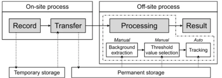
2.1.1 Conventional process flow
Figure 1 illustrates a typical process flow for droplet measurements. In brief, the process can be divided into
on-site and off-site steps. In the on-site step, the process initiates by recording droplets using a high-speed video camera which is fitted onto a microscope. The record-ing duration depends on several factors such as the speed of the droplets, droplet production frequency and num-ber of droplets to be evaluated. This in turn determines the frame rate to be used and the duration of the record-ing. In general, the frame rate has to be higher than the droplet production frequency to allow an accurate analy-sis. For instance, it takes 0.1 s to record 1000 frames at 10,000 frame per second (FPS) on 35 droplets generated at a production rate of 350 Hz. The recorded video is then transferred from the camera’s temporary storage to a per-manent storage such as computer hard drive or external memory storage. The time taken depends on the trans-fer speed and the writing speed of the video data. As an example, this process takes more than 5 s transferring 1000 frames, 520 × 64 pixels video data from a camera (Phantom Miro M310) without any video compression to a computer hard drive.
In the off-site image evaluation, the experimental videos first need to be processed before any droplet measurements can be extracted for further analysis. In this operation, it first involves extracting the background and the selection of an appropriate threshold value in order to convert the video into binary images. This step is usually done manually by inputting and selecting the appropriate parameters. The parameters are then checked by scanning through the video in the software to inspect the suitability. Next, the droplets are tracked and monitored to avoid repetition and dou-ble counting. This is done by analyzing each frame of the video. In each frame, the background is removed and the image is then converted into a binary image. The contours of the droplets are then identified from the binary image. After filtering the contours, each of them is compared and linked to one of the contours obtained from the previous frame. The time used in this process depends on the image recognition library and the efficiency of the coding. For instance, a MATLAB-based DMV video recognition soft-ware by Basu (2013) takes about 45 s (Windows 7 PC with Intel Core i7 M620 CPU) to process 945 frames of video with resolution of 520 × 64.
Temporary storage Permanent storage
Background
extraction value selectionThreshold Tracking
Transfer
Record Processing Result
On-site process
Manual Manual Auto
Off-site process
2.1.2 New process flow with ADM software
The study of the droplets characteristic in different flow fields or external conditions requires multiple experiments and repeated tests. Usually, tens or even hundreds of tests have to be performed diligently before one can understand and elucidate the unique experimental observation. When coupled with the above image processing technique, it usu-ally takes many painful months or even years before plau-sible conclusions are reached after the analysis. Recogniz-ing this, it is impractical and time-consumRecogniz-ing to perform the above process. The process is also highly inefficient as the droplet measurements can only be obtained after an off-site analysis. Therefore, rapid and automated droplet measurement software will address this inadequacy. We propose here a new process flow in Fig. 2 which allows droplet measurements to be carried out on-site and run automatically.
In order for the new process flow to be efficient and practical, we addressed three main bottlenecks that hamper the rapid measurement of droplets. We first identified and automated two main critical functions, namely the extrac-tion of background image and selecextrac-tion of threshold values. We then addressed the tracking speed of the droplets by optimizing the coding for tracking to enable a fast detec-tion and measurement system. The new process flow can be executed seamlessly and run on-site for rapid droplet measurements.
The first bottleneck to remove toward an automated and rapid measurement system is the extraction of background information. The implementation of an effective back-ground extraction operation (BEO) must (1) suit the char-acteristics of the droplet movement and (2) be universally applicable to different environments.
The automation of the binary threshold value selection (BTVS) operation suppresses the second bottleneck: by selecting its optimized value automatically from the opera-tion, the prominent contours from each video frames can be properly recognized by the software.
For most video conditions, the two operations described enable the software to track the droplets reliably.
Furthermore, an unmanned processing step drastically overcomes manual operation in terms of time and invari-ability of objective criteria for the selection of optimal parameters. Also, for most situations, finding the optimal parameters for video tracking resolve the other processing parameters such as erosion, dilation and advanced filtering measures. The two devised algorithms will be explained in detail in Sect. 2.2.
The third bottleneck entails the speed of our ADM software to run the two mentioned automated processing operations. In addition, the software must be able to track the droplet at a much higher image processing speed than the currently available software. To do so, our target is to achieve a tracking speed comparable to or higher than the transfer speed of video data. The viability of the new pro-cess flow is thus linked to that target. The improvement provided by the new process lies on the streaming of video data into a PC memory instead of transferring it to a perma-nent storage. As the I/O (input/output) speed of PC mem-ory is higher than a permanent storage, it allows simulta-neous video frame streaming from camera and access by ADM for the tracking step. For BEO and BTVS opera-tions though, the software accesses the temporary storage directly as the number of frames is small (about 100) and the frames are picked randomly.
By implementing the new process flow with the pro-posed ADM, the tracking speed is now limited by the transfer/streaming speed only, as the tracking speed is com-parable or faster than the transfer speed. This will further cut down the time spent on the whole process. Moreover, simultaneous streaming and tracking allow the software to stop the streaming after tracking sufficient number of drop-lets, which reduces the time taken even further.
2.2 Making processing step fully automated
2.2.1 Object‑based BEO
The background extraction operation (BEO) is the first basic step in the image processing for subsequent droplet measurements. Indeed, tracking the moving object (drop-let) accurately by the image processing software requires a background removal operation (BRO), which uses the extracted background by BEO (Gavrilova and Monwar 2013). By using a properly extracted background, BRO clears out permanent background features such as the chan-nel wall from every frame in the video. This eliminates the need for manual intervention to prevent those features from being tracked by the software.
Naturally, BEO can be done by simply taking the picture of the channel before the formation of droplet. However, the extracted background becomes obsolete once the image condition has been changed. For instance, a new BEO has
Streaming
Temporary storage PC memory
Background
extraction value selectionThreshold Optimizedtracking
Record Automated processing Result
Auto Auto Auto langi
s gni ma ert s pot S
Fig. 2 New droplet measurement process flow with automated
to be performed once the stage position or the lightning condition changes. New BEO is also needed; when the device has been used for an extended period of time, the channel walls may swell and deform due to the presence of organic solvents.
It is inconvenient and inefficient to stop the droplet formation process just for a new BEO whenever there is a change in the image condition. Fortunately, each of the video frames capturing the droplet generation already contains fractional information regarding the background image. Therefore, it is possible to perform BEO from a video, by combining the fractional information from a lim-ited number of video frames in order to form a complete background image.
Basu (2013) suggested a statistical survey approach on each of the pixels in the video frames in order to perform BEO from a video. By performing the survey, the statistics of the intensity value for each of the pixels across the sam-pled frames can be determined. A new image can then be formed by setting each of the pixels with the intensity value accordingly to the statistical data such as average, mode, median, minimum and maximum.
According to Basu (2013), the new image generated by setting the intensity values to their modes can represent the background correctly for most of the time. However, we find that this method is not ideal for all situations as it fails to extract a proper background for droplet generated at low flow rate ratio (dispersed phase to continuous phase). This curbs the universality of the method to perform BEO, where the study of droplet generating at low flow rate ratio is common. As this limitation can impede the automation of the processing step, we developed a new and more uni-versal object-based BEO that suits the characteristics of the droplets traveling in microchannel.
As illustrated in Fig. 3, we developed an object-based BEO that is derived from a modified statistical method. The operation starts by generating an average image (A1) using 40 randomly selected frames (F1–F40), where 40 is a number that balances BEO accuracy with operation speed and cost as described next. Then we remove the non-back-ground regions in A1 by using an operator h which extracts fragments of background regions from randomly selected frames (F41–F80). Image R1 shows the result of the first iteration of the operator h on image A1 with image F41. The area of the non-background regions in image A1 is reduced after h(A1, F41, A1) operation. The area is reduced further in the second iteration applying h(R1, F42, A1), as shown in image R2. After 40 iterations, the area of the non-background regions is reduced, as shown in image R40. Further iterations produce exponentially decaying, negligi-ble improvements in background extraction.
Operator h is crucial for the effectiveness of the pro-posed object-based BEO. The operation discriminates
between the moving objects and the background in the randomly selected video frame. This operator determines the regions to extract from the randomly selected video frame and patches them on the average image. The result of applying h on images with 256 gray intensity levels is illustrated in Fig. 4. We use the transformation of image R1 to R2 by h(R1, F42, A1) as an example to show how the operator works in detail.
The operation starts by performing a preliminary back-ground removal (PBR) procedure on image F42 using A1 as an average image. The formula used for the procedure is shown in Eq. (1), where F is the image to perform PBR while A is the average image.
(1a) D1ij=f (Fij, Aij)= 255, l2(Aij)≤ 0 or l2(Fij) > l2(Aij) 0, l2(Fij) <0 255 ×l2(Fij) l2(Aij), otherwise (1b) l2(Iij)= 245(Iij− Imin) Imax− Imin + 10 F1 F3-F40 Aver age(F1-F40) h(A1, F41,A1 ) F43-F80 h(R1, F42, A1 ) 38 iterations of h F2 R1 R2 R40 F42 F41 A1
Fig. 3 Overview of object-based background extraction operation
(BEO), where F1–F80 are randomly selected frames, A1 is the aver-age of the frames, while R1–R40 are the frames with reduced non-background areas g(D1) B1.*F4 2 R1*.B 2 c(B1) M 1+M 2 f )1 A, 24 F( D1 B1 M1 B2 M2 R2 R1 A1 F42 h(R1, F42, A1)
Fig. 4 Transformation of image R1–R2 using operator h on the
image vector {R1, F42, A1}, i.e., R2 = h(R1, F42, A1), during the execution of object-based BEO. D1 is the frame with removed back-ground, B1–B2 are the binary images, and M1–M2 are the frames overlapped with masks
Fij, Aij and Iij are the pixel intensity matrices of the
cor-responding images. The Imin and Imax used in Eq. (1b) are
the minimum and maximum pixel intensity value of image
F1–F40 found out during the generation of image A1. l2
function is used to optimize the intensity range. Note that the minimum pixel intensity value yielded is 10 in order to avoid oversensitive division operation at single digit value of intensity. As shown in Fig. 4, image D1 is the result after performing PBR on image F42. Here we use background division instead of subtraction for the background removal procedure as it is more robust to illumination changes (Izquierdo-Guerra and García-Reyes 2010) and uneven illumination. This is important to produce consistent results under a variety of situations. Background division is also effective for the procedure that uses an imperfect back-ground image like A1.
Operation is then continued by converting image D1 into a binary mask B1 (see Fig. 4). The g procedure used for the conversion marks the moving objects in image F42 as dark regions. The procedure starts by converting image D1 into a binary image with 0 (dark) or 1 (bright) in pixel inten-sity value. The bright inner areas of the binary image are then filled up to mark out the moving objects. Afterward, we expand the dark areas with a scale relative to the width of their minimum bounding rectangle. The expansion is done to cover the shallow shadows of droplets that are not bounded by the initial dark areas.
The produced binary mask B1 is then multiplied with image F42 element by element to cover the moving objects in the image, as shown in image M1. Conversely, image
B2, a complimentary binary mask of B1 is multiplied with R1 element by element to produce M2. Afterward, addition of M1 with M2 produces image R2, [the result of the operator h on the image vector {R1, F42, A1}, i.e.,
R2 = h(R1, F42, A1)] has a closer representation of the
real background compared to R1. Finally, the BEO process can be formally defined as the sum of an average operation over an image vector {F[I]}I=1,...,n, where n is a properly
selected order (here, n = 40), plus an operator H composed of n nested operators h(R[J − 1], F[J + n], A1) on the image vector {F[J + n]}J=1,...,n, starting with the average
image R0 ≡ A1.
2.2.2 Automated BTVS
An image is usually converted into a binary image for contour recognition. Before binary image conversion, we need to select a suitable binary threshold value as it affects the quality of the contour recognition. The suit-able binary threshold value is unique for each video as the channels are captured under a variety of lightning condi-tion, background and degree of transparency. This makes the video, from one to the other, to have different edge
contrast of droplet outlines. Therefore, binary threshold value selection (BTVS) is another essential operation in the processing step. The operation ensures the exact con-tours to be recognized from the converted binary image and that conforms closely to the outlines of droplets. BTVS is also vital for the reliability of droplet tracking and the accuracy of the droplet measurement. By using the optimal threshold value, we could also reduce the need to perform dilation or closing operation to join the disconnected traced droplet outlines from an improperly processed binary image.
The currently available droplet measurement software or DMV requires the user to perform BTVS manually. This is done by changing the value of binary threshold and check-ing the converted binary image. As the selection is done visually, the selected value is different not only from one user to the other but also from time to time within the same user. In order to resolve the issue, we have developed a method to perform BTVS automatically. The method ena-bles automatic selection of an optimum threshold value with high repeatability.
Our automated BTVS starts by selecting one frame from a video to produce multiple binary images converted using different threshold values. As the frame is an image with gray intensity level from 0 to 255, we convert the frame into 254 binary images using threshold values from 1 to 254 in one operation of automated BTVS. Afterward, con-tour recognition is done on each binary image, ascending from the binary image converted at the lowest threshold value (T = 1) to the highest threshold value (T = 254). The contours recognized at each threshold value are grouped together according to their centroids using a nearest neigh-bor search. By the end of the nearest neighneigh-bor search at
T = 254, each group will contain at least one or multiple contours with similar centroid, collected at subsequent threshold values.
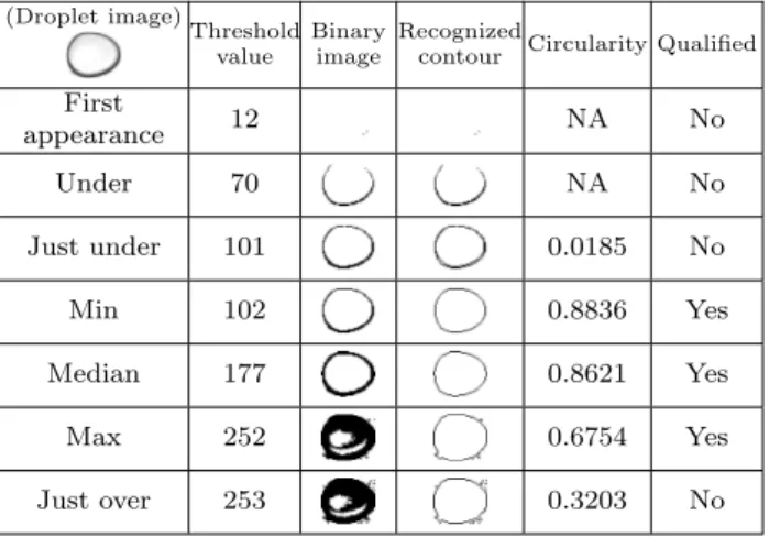
Table 1 shows an example that illustrates the process of the automated BTVS on the droplet image in the table. The outline of the droplet first appears at binary image
T = 12 as two dots. The outline becomes more prominent when the threshold value increases, as shown in the binary images in Table 1. After performing filtering of contours and nearest neighbor search, there is only one group of contours with similar centroids and recognized from binary images converted with increasing threshold value (T = 102 to T = 252). The recognized contours from binary image
T = 101 and below are unqualified either for not reach-ing the minimum area (e.g., small contours in T = 12 and
T = 70) or with circularity value (4π × Area/Perimeter2)
lesser than 0.5 (e.g., disconnected contours in T = 70 and
T = 101). The recognized contours from binary image
T = 253 and T = 254 are also unqualified as the spiky con-tours have low circularity values.
After sorting the filtered contours into groups, we know from each group the range of threshold value with features recognizable as qualified contours. In situations where there is only one group of contours, the automated BTVS will select the median of the range as the suitable threshold value. For the example in Table 1, the outline of the drop-let image is recognizable in the range from T = 102–252. Thus, the median value, 177, will be selected.
In order to increase the repeatability of the automated BTVS, we would need to sample more than a droplet image. Our policy, outlined in the following, will be sub-sequently discussed in detail in Sect. 3.2. By increasing the sample size, there will be more groups of qualified contours. Furthermore, as more frames are sampled in the automated BTVS, it is unavoidable to have groups of contours that have small range of threshold value, repre-senting the non-prominent features such as a faint back-ground object. The groups of this kind can be excluded by setting a minimum acceptable range, such as 20 set in ADM software. We can finally select a suitable threshold value from the remaining groups by analyzing the range of threshold values of each group. We select the top 50 % groups of the larger range and collect the medians of their range. The final value will be the median of the collected medians. The lower 50 % groups are excluded from the collection as they may contain groups of shorter range recognized from the droplets near the edge or the extended fingers right before separating from the dis-persed phase.
2.3 Integrated program with ADM software and camera SDK
After implementing object-based BEO and automated BTVS in ADM software, we have made the processing step fully automated, together with tracking operation. Besides, the implementation also ensures proper tracking
of the moving object by ADM software according to the characteristic of the video, under most of the situations. The whole measurement process flow can then be com-puterized by developing an integrated program. As shown in Fig. 5, the two main modules used in the program are the software development kit (SDK) provided by camera manufacturer and ADM software. The former module is used to control the high-speed camera and retrieve the data from it, while the latter is to perform the processing step automatically.
As far as we know, DMV by Basu (2013) is the only publicly available droplet tracking software, which is written in MATLAB. The software has not been opti-mized for high performance as mentioned by Basu (2013). Apart from MATLAB, OpenCV is another popu-lar image processing library. OpenCV library is written in optimized C, and its performance can be enhanced by the use of multicore processors (Nuno-Maganda et al. 2011). Due to this, OpenCV consumes lesser CPU time than MATLAB for basic image processing operations (Matuska et al. 2012). OpenCV is also widely used and adopted in many research fields as the tool for real-time computer vision that requires high processing speed (Bradski 2008). Therefore, we use the OpenCV library for our ADM software in order to achieve rapid tracking of droplet movement.
We wrote ADM software from ground up in Visual C# using OpenCV through Emgu CV, a wrapper to the OpenCV library. Visual C# is adopted for efficient Win-dows GUI development, and it will help to design instan-taneous result feedback without consuming large computer resources. We optimized the coding to match or surpass the video data transfer speed. The simplified architecture of the integrated software is illustrated in Fig. 5. Thread con-trol is required for program features such as simultaneous streaming and tracking and instantaneous visual feedback. Resource management is particularly important for inten-sive processes such as frame streaming and tracking. Some of the results are represented by graph plotting using Zed-Graph, an open-source class library and user control for drawing 2D Line, bar and pie charts.
ADM software (C#) EMGU CV (C#) OpenCV (C/C++) Image processing Presentation BEO BTVF Tracking
Result Windows GUI (C#) ZedGraph (C#) Camera SDK (C#) Camera control Frame reading Frame streaming Integrated program Thread control Resource management
Fig. 5 The simplified architecture of the program integrating camera
SDK and ADM software
Table 1 The process data of automated BTVS on a droplet image
(Droplet image)Threshold
value Binaryimage Recognizedcontour Circularity Qualified
First appearance 12 NA No Under 70 NA No Just under 101 0.0185 No Min 102 0.8836 Yes Median 177 0.8621 Yes Max 252 0.6754 Yes Just over 253 0.3203 No
3 Results and discussion 3.1 Object‑based BEO
3.1.1 Choosing a suitable method for PBR procedure
As mentioned in Sect. 2.2.1, operator h is crucial for the effectiveness of object-based BEO. The operator patches part of the non-background regions in an image with the background in a newly selected random image. This opera-tion is made possible by having an effective PBR proce-dure based on an average image, which is an imperfect background. The result of the procedure is shown in Fig. 4, where the background in image F42 is removed using image A1 to produce image D1 under the f(F42, A1) proce-dure. Other methods have also been tried for the PBR pro-cedure before adopting method f stated in Eq. (1) for the procedure. The methods are r1, r2and r3, which are shown
in Eq. (2). For the symbols used in the equations, Fij is
the image to perform PBR, Aij is the average image, l1 is a
leveling function to optimize the range of intensity value, while Imin and Imax are the minimum and maximum
inten-sity value, respectively. Imin and Imax are surveyed during
the generation of the average image.
Method r1 is a standard background subtraction. The
pixel in image r1(F, A) takes the middle value (128)
when Fij = Aij. The pixel intensity is darker (<128) when
Fij< Aij while lighter (>128) when Fij> Aij. Method r2
is an absolute background subtraction. The pixel in image
r2(F, A) is 255 when Fij= Aij. The pixel intensity becomes
darker (<255) whenever there is a difference between Fij
and Aij. Method r3 is similar to r2, but the pixel intensity
remains 255 when Fij > Aij.
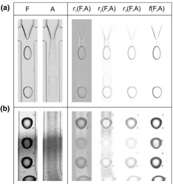
As shown in Fig. 6, all the methods are able to remove the outlines of the channel wall effectively. Interestingly, the images produced by method r3 and f do not have the
shad-owy droplet outline shown in image inherited from image A. This is because the methods do not discriminate the change for Fij > Aij. Methods r3 and f are especially suitable for
capturing droplets because the droplet outlines are darker than the background. Method f is preferred than method r3,
as the images produced using f method shows the droplet outlines more clearly and in higher contrast. Additionally, (2a) r1(Fij, Aij)=128 + 0.5l1(Fij)− 0.5l1(Aij) (2b) r2(Fij, Aij)=255 − |l1(Fij)− l1(Aij)| (2c) r3(Fij, Aij) = 255, l1(Aij)− l1(Fij) < 0 255 − (l1(Aij)− l1(Fij)), otherwise (2d) l1(Iij)= 255(Iij− Imin) Imax− Imin
method f is insensitive to the lightning distribution, as exem-plified in case (b) of Fig. 6. For this case, the outline of droplet in the darker region is much clearer from the image produced using method f than the one using method r3.
After performing the assessment on several other vid-eos using the above-stated methods, we chose method f as the PBR procedure in BEO. Method f is able to produce consistent result in a variety of lightning conditions, with high contrast images showing the droplet outlines clearly. This allows the use of a fixed threshold value, independent of the video condition, in using g procedure to produce a binary mask for operator h.
F A r1(F,A) r2(F,A) r3(F,A) f(F,A) (a)
(b)
Fig. 6 Comparison of four different methods for PBR procedure
(r1,r2,r3,f) on a video A—the experimental setup is discussed in
Sect. 3.3.1 and b video B—the experimental setup is discussed in Sect. 3.3.2 Video Object based BEO Mode BEO (a) (b) (c) (d)
Fig. 7 BEO on different types of video. a Droplet splitting, b droplet
formation, c droplets traveling under channel with variety lightning distribution and d bubble formation
3.1.2 Application of BEO on different videos
Our proposed object-based BEO has been tested on differ-ent types of video. As shown in Fig. 7, the videos include (a) droplet splitting, (b) droplet formation, (c) droplets traveling under channel with non-homogeneous lightning distribution, and (d) bubble formation.1 According to the test results, object-based BEO is able to extract the correct background for droplets captured under different situations. The test result is also compared to mode BEO (a statistical method, by setting the intensity values to their modes), which highlights benefits of object-based BEO. Mode BEO fails to generate the correct background for from video (a), (c) and (d), as some of the intensity values are from the moving objects. This generates the unwanted darker or lighter tails in the extracted backgrounds.
3.2 Automated BTVS
3.2.1 Application of automated BTVS
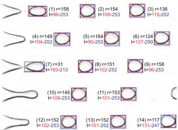
Figure 8 shows the result of our automated BTVS opera-tion applied on a video capturing the droplet formaopera-tion. The video is the same as the one used in case (b) in Fig. 7. The operation is done on an image combining five frames from the video. Each frame is selected randomly from the video and performed with background removal before the combination. Five frames are used to increase the prob-ability of capturing a droplet in the field of view while not reducing the speed of BTVS operation. There are 14 groups of qualified contours recognized from the image under the operation. Each group is labeled in the figure with a pair of rectangles in red and blue. The red rectangle is the bound-ing rectangle for the qualified contour recognized at the lowest binary threshold value from a group, while the blue one is at the highest value. For instance, object (2) is recog-nizable as a qualified contour from the image starting from threshold value of 100 until 253, with range of 154.
Table 2 lists the groups recognized from the video using our automated BTVS. As all the sizes of the range are larger than 20, none of the groups are removed from the list. Each group is then ranked according to the size of range, from biggest to the smallest. Afterward, the top 50 % groups in terms of the size of range will be included in the selection of a suitable threshold value. For this case, groups (3), (4), (6), (7), (8), (10) and (14) are excluded. Object (7) has the smallest in range as it is recognized from the extended finger right before separating from the dis-persed phase. Object (14) is the next smallest recognized from a droplet near the edge of the frame.
1 ADM can also be used to measure bubbles.
The medians of the included groups are then collected. Finally, by computing the median of the collected medians, automated BTVS selects value 176 for the threshold value. In order to evaluate the quality of the selected threshold value, we compare the object images and their converted binary image at the selected threshold value. We list the object images, binary images and recognized contours
(1) r=158 t= -96253 (2) r=154t=100-253 (3) r=138t=115-252 (4) r=149 t=104-252 (5) r=164t= -90253 t=(6) r=124127-250 (7) r=31 t=183-213 (8) r=151t=102-252 (9) r=158t= -96253 (10) r=145 t=109-253 (11) r=153t=101-253 (12) r=152 t=102-253 (13) r=152t=101-252 (14) r=117t=131-247 Fig. 8 The groups of qualified contours recognized from the image
under automated binary threshold value selection (BTVS)
Table 2 Data of the groups of recognized contours
Group Max Min Range Rank T Object
image Binary atT=176 Contour atT=176 Qualifiedcontour
(1) 96 253 158 2 174 Yes (2) 100 253 154 4 176 Yes (3) 115 252 138 11 - Yes (4) 104 252 149 9 - Yes (5) 90 253 164 1 171 Yes (6) 127 250 124 12 - Yes (7) 183 213 31 14 - No (8) 102 252 151 8 - Yes (9) 96 253 158 2 174 Yes (10) 109 253 145 10 - Yes (11) 101 253 153 5 177 Yes (12) 102 253 152 6 177 Yes (13) 101 252 152 6 176 Yes (14) 131 247 117 13 - Yes
The median is collected only from the top 50 % of the group in terms of size of range. Therefore, we find out the median only for the rank 7 or higher groups
according to their associated groups in Table 2. We find the binary images generated at the selected threshold value (176) represent the object outlines correctly. Addition-ally, the recognized contours from the binary images are able to trace the outlines of the objects closely. Among the contours generated at T = 176, contour from group (7) is unqualified automatically as it is recognized from an object with a broken outline. The contour has circularity value lower than 0.5. The exclusion of the group (7) at T = 176 is consistent to what we want as it is not yet a droplet.
3.2.2 Repeatability of automated BTVS
The automated BTVS operation is sampled from image combining five randomly selected frames from a video. The probability of capturing at least one droplet is near def-inite with five frames while not compromising the comput-ing performance. As the frames are randomly selected, the determined threshold value can fluctuate from one execu-tion of the operator to the other. Here, we study the fluctua-tion of the value and its implicafluctua-tion to the measured droplet area on the same video. Figure 9a shows the histogram of the threshold value obtained using the automated BTVS for 100 times. The threshold value fluctuates between 174 and 178. The measured droplet area changes slightly from one threshold value to the other, from 1133.3 to 1136.1 pixel2 .
For this case, the standard deviation of the measured area is 0.7427 pixel2, or with coefficient of variation (CV) of
0.0655 %. This value is small enough to ensure high repeat-ability for the measurement.
3.3 Measurement result
3.3.1 Droplet generation
Our ADM software has been used to perform droplet measurement on a typical microfluidic droplet generation process. We captured the process of droplet generation by a polydimethylsiloxane (PDMS) device with a cross junc-tion design (channel width and height of 100 and 45 µm, respectively). The device was fabricated using standard soft lithography techniques (Duffy et al. 1998). As shown in Fig. 9b, we form water droplets in oil by flowing deionized water (dispersed phase) to the central channel of the cross junction and mineral oil (continuous phase, Sigma-Aldrich M5904 with 5 % w/w surfactant; viscosity η = 30 mPa s; surface tension γ = 33 mN m−1) to the two side channels.
The volumetric flow rates are maintained using syringe pumps (neMESYS, Cetoni) at 200 µL/h for the dispersed phase while 1000 µL/h for the continuous phase. We cap-ture the droplet generation using a microscope (BX51, Olympus) fitted with a high-speed camera (Miro M310, Phantom). After maintaining the flow rates for an hour,
30 droplets are captured and measured under the new pro-cess flow with ADM software. The average area, speed and perimeter were found to be 4503.1 µm2, 100.51 mm/s and
255.7 µm, respectively. The CVs for the three values are all lesser than 0.2 %. Right after measuring directly using ADM, we also recorded a short video capturing 30 droplets for manual and DMV measurement.
We check the accuracy of our measurement by compar-ing the deduced flow rate from our measurement data to the set flow rate at the pump. The flow rate is deduced using Eq. (3), together with the estimated droplet volume equa-tion, Eq. (4), for droplet in a channel with rectangular cross section (Steijn et al. 2010).
The Q, f and V values are the deduced flow rate, drop-let generation frequency and dropdrop-let volume, respectively, while h, A and p are the height of channel, top-view area and perimeter, respectively. As the measured droplet gen-eration frequency is 353.7 Hz, the corresponding deduced flow rate is 187.3 µL/h, which do not deviate much from the set flow rate (200 µL/h) at the pump for the dispersed (3) Q = fV (4) V = hA − 2p h 2 2 1 −π 4 (a) (b)
Fig. 9 a Histogram of the obtained threshold value in 100 times
using automated BTVS algorithm. b Droplet generation device. The schematic is not drawn to scale
phase. This deviation can be attributed to the volume equa-tion used, which may need appropriate correcequa-tion factors to account for the roundness features in the direction nor-mal to the plane of view in this case. Other factors such as inaccuracy in the measurement of channel height, recogni-tion of contour and syringe pump may also contribute to the deviation. Here, the length-average error is only 2.17 % (cube root of the ratio of the deduced and the set volume flow rate), which is an acceptable value.
Figure 10 shows the screenshot of our ADM software. We are able to trace each of the recognized contours, grouped accordingly using nearest neighbor finding, after tracking of droplets. For the plotting of data, we list com-mon parameters needed in droplet measurements. For the plots, (a) is time against group ID (unique serial number to the group with recognized contours classified as from the same droplet), illustrating the time and duration of the occurrence of each droplet, (b) is y position against x posi-tion, which shows the imperfectness of the stage align-ment and also highlights the deviation of droplet movealign-ment from the centerline due to some defects in the channel, (c) is contour perimeter against time, showing the trend of the dimension across the time, and (d) is a histogram showing the distribution of top-view droplet areas.
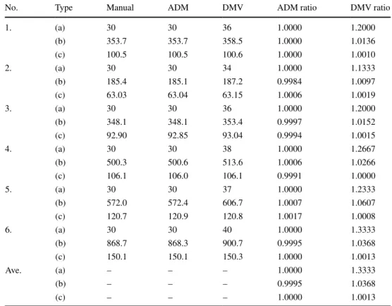
The recorded video of the droplet generation is measured manually and validated using both DMV and ADM. Man-ual measurements were taken by inspecting each individMan-ual frames of the recorded video. The comparison between each measurement is shown in Table 3, row no. 1. First, the number of droplet detected by DMV is higher than both the manual analysis and ADM. Here, ADM is more accu-rate than DMV due to the enforcement of a tighter drop-let discrimination rule. A dropdrop-let is counted only when it is traced from its separation from the liquid finger to the disappearance from the defined region of interest. This rule
is implemented to prevent double counting of droplets and also to ensure a more accurate measurement when comput-ing the average. As a result, the first three droplets and the last three droplets counted by DMV are disqualified when counted by ADM. The droplet generation frequency and the droplet speed calculated by DMV is higher due to the inclusion of the unqualified droplets. In the same table, row no. 2–6 shows the measurement of droplet generation using the same setup with different flow conditions. Again, the measurement performance is consistent with row no. 1.
3.3.2 Droplet splitting
ADM software has also been used to perform measure-ments on droplet splitting. The device used in this video is a PMMA device fabricated by injection molding (Yu et al. 2014). The channel width and height are both 200 µm. The dispersed phase is deionized water, while the continuous phase is light mineral oil (330779, Sigma-Aldrich) with 2 % w/w surfactant (Span 80, Sigma-Aldrich). The volu-metric flow rates are maintained using syringe pumps at 35 µL/min for the dispersed phase while 100 µL/min for the continuous phase. The frames of the video are shown in image F41 and F42 of Fig. 3.
ADM software has a special image box for visual feed-back in order to monitor the tracking effectively. This fea-ture is also suitable for the splitting case. The software updates the special image box with a representative con-tour from its concon-tours group once the group exits from the visible region. The representative contour is the contour at the half of the group’s visible period. For example, contour at frame 20 is chosen from a group appearing from frame 11–29. The contour is then filled with the color according to the group number and drawn on top of the image box, as shown in Fig. 11a. As the image box is not cleared for each draw, we still can see some remnant contours around the three filled contours. This feature helps us to have a snapshot of the history of tracking. Erroneous tracking due to the factors such as selection of wrong binary threshold value can be easily spotted as the filled contours are scat-tered around the channel, as shown in Fig. 11b.
Figure 11 also includes some useful plot generated instantaneously from ADM software. Plot (c) tracks the centroids of all contours with their according to their group color. This is to show the contours are traced and grouped properly during the tracking process. Plot (d) shows the entation of droplet movement against x position. The ori-entation of two newly split droplets differ the most. They return to near 0◦ gradually as they move along the x
direc-tion. Plot (e) shows the changing of the top-view area of droplets. The area increases before the splitting and drop significantly after the splitting. Plot (f) shows the histogram of the top-view droplet areas. The count for the smaller Fig. 10 Screenshot of our ADM software with data plots: a time
against group ID, b y position against x position, c contour perimeter against time and d histogram of droplet areas
area is 108, while the bigger area is 55. By counting the last two split droplets excluded from the data as they are still in the viewing region, the count for the smaller area is 110, which makes it exactly twice the count of the bigger area.
The recorded video of the droplet splitting has also been measured manually for validation. The split droplets are measured according to the locations of the split chan-nel (upper and lower). The comparison is shown in Table 4. For the comparison, we deduce the dispersed flow rate by using Eq. (3). As the split droplets are unconfined under the channel (diameters smaller than the width and height of
the channel), the droplets are assumed to be perfect spheres with volume of V = (4/3)πr3. The r of the equation is
deduced from the average area (A) using r =√A/π.
The deduced dispersed flow rate (Qd) is found by adding
the deduced half Qd from the upper and lower channel. Both
the deduced Qd by ADM and DMV are close to the imposed
dispersed flow rate (35 µL/min) by the setup. The meas-urements for ADM are found to be within a ratio (0.9634– 1.0038). The measurements for DMV are found to be within a ratio (0.9833–1.0427). Here, it is reasonable to conclude that both software are fairly accurate in the above measurements. 3.4 Features of ADM
3.4.1 Speed
The integrated program is run on a PC with Intel Core i7 CPU (M620) on Windows 7. The time taken for the pro-gram to execute the object-based BEO on droplet genera-tion video (520 × 64 pixels, Lagarith lossless video codec) is about 0.5 s, while the automated BTVS takes about 1.1 s. For the tracking step, the program takes about 2.9 s to process 945 frames of the video, with visual feedback showing the tracking process and instant data plotting. On the other hand, DMV takes about 45 s to process the same video without visual feedback. When the visual feedback is enabled, the time taken increases to about 380 s. Therefore, our ADM software is able to process the video more than Table 3 ADM measurement
result compared to DMV (droplet generation) with different measurement types— (a) number of droplet, (b) frequency (Hz) and (c) speed (mm s−1)
No. Type Manual ADM DMV ADM ratio DMV ratio
1. (a) 30 30 36 1.0000 1.2000 (b) 353.7 353.7 358.5 1.0000 1.0136 (c) 100.5 100.5 100.6 1.0000 1.0010 2. (a) 30 30 34 1.0000 1.1333 (b) 185.4 185.1 187.2 0.9984 1.0097 (c) 63.03 63.04 63.15 1.0006 1.0019 3. (a) 30 30 36 1.0000 1.2000 (b) 348.1 348.1 353.4 0.9997 1.0152 (c) 92.90 92.85 93.04 0.9994 1.0015 4. (a) 30 30 38 1.0000 1.2667 (b) 500.3 500.6 513.6 1.0006 1.0266 (c) 106.1 106.0 106.1 0.9991 1.0000 5. (a) 30 30 37 1.0000 1.2333 (b) 572.0 572.4 606.7 1.0007 1.0607 (c) 120.7 120.9 120.8 1.0017 1.0008 6. (a) 30 30 40 1.0000 1.3333 (b) 868.7 868.3 900.7 0.9995 1.0368 (c) 150.1 150.1 150.3 1.0000 1.0013 Ave. (a) – – – 1.0000 1.3333 (b) – – – 0.9995 1.0368 (c) – – – 1.0000 1.0013
Fig. 11 The result of droplet splitting measurement taken from
screenshot of the ADM software a visual feedback for correct track-ing, b visual feedback for erroneous tracking at low binary threshold value, c y position against x position of centroids, d droplet move-ment orientation against x position, e changing of droplet area against x position and f histogram of droplet area
15 times faster than the MATLAB-based DMV program, even when the ADM is enabled with the visual feedback and data plotting for the tracking of the droplets.
As the tracking speed (∼326 FPS) is much faster than the streaming speed from camera (Phantom Miro M310) (∼150 FPS) at the given resolution, the ADM software has been combined with the SDK of the camera to perform tracking operation while streaming from the camera. This enables rapid tracking of droplet using the new process flow proposed in Fig. 2. However, the software is still able to operate separately without the SDK using the conven-tional process flow by loading avi format video files.
Table 5 shows the time taken to perform different sets of tasks for droplet measurement. Each of the two videos is given three different sets of tasks that emulate the pos-sible strategies to be adopted for measurement of droplets. The first two sets perform only the record and transfer steps on-site. Processing step (BEO, BTVS and tracking) is done off-site after transferring the videos, as stated in the con-ventional process flow. The former uses DMV software to do processing step, while the later uses our ADM software. Set 3 uses the new process flow to perform all the steps of droplet measurement on-site, by making streaming and tracking working in simultaneously.
It is obvious from the result that set 1 requires the long-est time to finish both videos. The tracking step consumes the most time. For set 1, the time taken for the BEO and BTVS is only estimated as they are done manually and depends on the experience of the operator. We assume more time will be taken in the BEO for the second video as the operator needs more time to choose the other suitable background extraction scheme, after failing to extract the background using the default mode scheme.
The second set saves a lot of time for both videos com-pared to set 1. This is because the BEO and BTVS can be done automatically and the tracking operation is much faster. Set 3 consumes the least time. However, as the BEO and BTVS are taking the video frames directly from the camera, the times are extended for those operations com-pared to set 2. Furthermore, the tracking time is limited by the streaming speed from the camera. The streaming speed is slightly slower than the transfer speed in first two sets, as it takes some time to initiate the buffer for the streaming. Overall, the time taken in set 3 is still quicker than set 2, and comparable to the transfer speed.
3.4.2 Additional features
Apart from speed improvement, ADM also comes with a batch processing feature. This feature is especially helpful for automated mass measurements of droplets. The batch processing function processes each of the video files in a list automatically. ADM also measures more droplets param-eters than DMV. Besides the droplet paramparam-eters in DMV, ADM measures an additional three important parameters. The additional parameters are advancing/receding angle and droplet deformation which are critical for understand-ing the physical characteristic of droplets. These parameters are also useful to characterize and understand the droplet behavior in different conditions. Furthermore, ADM has an advanced option which allow users to modify the process-ing parameters to tailor to one needs. The contour history review for spotting unusual tracking phenomena is also included to allow users to check for abnormalities.
The important features of ADM are as follows: (a) more than 15 times faster than the MATLAB-based DMV Table 4 ADM measurement result compared to DMV (droplet splitting)
The split droplets are measured according to the locations of the split channel (upper and lower) a Not including unqualified droplets
b Average value from upper and lower measurement
c Estimated from dispersed flow rate using Eq. (3), by assuming V = (4/3)πr3, A = πr2
d Equivalent diameter, found from area using D = 2√A/π
Measurement Manual ADM DMV ADM ratio DMV ratio
Upper Lower Upper Lower
Number of droplet 54 54 54 54a 54a 1.0000 1.0000 Frequency (Hz) 165.34 165.34 165.34 165.48a 165.36a 1.0000 1.0001–1.0008 Speed (mm s−1) 40.532b 40.474 40.685 40.800 40.877 0.9986–1.0038 1.0066–1.0085 Area (μm2) 17,651c 17,218 17,356 18,063 18,149 0.9755–0.9877 0.9833–0.9916 Diameterd (μm2) 149.91c 148.06 148.65 151.65 152.01 0.9877–0.9916 1.0116–1.0140 Deduced volume (pL) 1.7640 1.6995 1.7200 1.8261 1.8392 0.9634–0.9751 1.0352–1.0426 Deduced half dispersed flow rate (μL/min) 17.500 16.860 17.064 18.131 18.248 0.9634–0.9751 1.0361–1.0427
program. ∼3000 frames in 10 seconds (520 × 64 pixels, Lagarith lossless video codec), (b) automated batch pro-cessing from a list of video files, (c) a total of 24 param-eters including three new features—advancing/receding angle and droplet deformation, (d) user-defined image pro-cessing parameters and (e) contour history viewer to review tracked objects and spotting abnormalities.
Different from DMV, which is only available to selected requests, our ADM is available freely from the ADM web-site (ADM 2015). A tutorial and guide are also available to provide a clear and concise usage on the software. The software can also be used as a standalone without the inte-gration with the camera SDK.
3.4.3 Limitations
Currently, the ADM software still inherits certain limita-tion inherent in the image processing technology. As dis-cussed by Basu (2013), the video resolution determines the accuracy and speed of image processing. Therefore, we still need to choose a suitable resolution that addresses the trade-offs in ADM. The current ADM software still has dif-ficulty in processing droplets that are touching each other. Although it is still possible to tune the threshold value and change the contour recognition algorithm to accommodate this situation, we do not include this feature as the accuracy of measurement will be severely compromised.
In order to allow the ADM system to perform properly, users are advised to adjust the frame rate of the camera so that it captures the movement of droplets with distance lesser than ten pixels between two frames. Users are also advised to optimize the microscope focus and lighting conditions to capture a clear contour of the droplets. This measure will provide a sharp contrast between the droplets and the background.
4 Conclusions
The main bottlenecks hampering the currently available software to perform in situ vital, rapid and automatic measurement on droplet-based microfluidics have been identified and successfully addressed. First, the processing step has been automated, and second, the droplet meas-urement software has been redesigned to generate auto-matic, real-time output at a speed overcoming that of video transfer.
Automated processing step has been achieved using a newly developed object-based background extraction oper-ation (BEO) and automated binary threshold value selec-tion (BTVS) operaselec-tion. The new object-based BEO was found to be more effective, adaptive and general than the current BEO in extracting the correct background from traveling droplet videos. Automated BTVS, on the other hand, was able to adaptively select a near optimum thresh-old value that allows close tracking of droplet outlines.
Automated droplet measurement (ADM) software has been developed based on OpenCV image processing library that has much higher throughput than currently available software. The process speed (∼300 FPS) was found to be higher than the transfer speed (~110–150 FPS) even when the visual feedback is enabled. ADM is also validated by comparing with both manual analysis and DMV.
Subsequently, to shorten the total time taken on droplet measurement even further, we integrated the newly devel-oped ADM software and camera SDK together in a new process flow. This was done by performing video transfer/ streaming simultaneously with video processing.
The total time for the droplet measurement using the integrated software was found significantly shorter than using the old process flow with DMV software (9.2 vs ∼61.1 s, 16.7 vs ∼100.1 s). Our process flow timing is Table 5 Time spent for different sets of tasks emulating the possible strategies to be adopted for measurement of droplets
The total times with bold are done with DMV, while the italic times are done with ADM
Video Droplet generation Droplet splitting
Set 1 2 3 1 2 3
On-site measurement No No Yes No No Yes
Process Flow Old Old New Old Old New
Software DMV ADM ADM DMV ADM ADM
Duration (s)
Record 0.1 0.1 0.1 0.4 0.4 0.4
Transfer 6.3 6.3 0.0 13.1 13.1 0.0
BEO ~2.0 0.5 1.1 ~7.0 0.6 1.4
BTVS ~8.0 1.1 1.2 ~8.0 1.1 1.1
Tracking (& streaming) 44.7 2.9 6.8 71.6 3.6 13.8
even comparable to the ones without droplet measurement (6.4 s, 13.5 s). Our ADM software will be publicly released for free. The software can be used on an avi video file, without the need to integrate the camera SDK.
5 ADM website
ADM software is available at http://a-d-m.weebly.com. Acknowledgments The authors gratefully acknowledge the
research support from the Singapore-MIT Alliance (SMA) program in Manufacturing Systems and Technology (MST) and the Singapore Ministry of Education (MOE) Tier 2 Grant (No. 2011-T2-1-0-36). Z.Z. Chong would also want to thank the support of Nanyang Techno-logical University Research Scholarship.
References
ADM (2015) Adm website. http://a-d-m.weebly.com/. Accessed 01 July 2015
Basu AS (2013) Droplet morphometry and velocimetry (DMV): a video processing software for time-resolved, label-free tracking of droplet parameters. Lab Chip 13(10):1892
Bradski G (2008) Learning OpenCV: computer vision with the OpenCV library. O’Reilly, Sebastopol
Brouzesa E, Medkova M, Savenelli N, Marran D, Twardowski M, Hutchison JB, Rothberg JM, Link DR, Perrimon N, Samu-els ML (2009) Droplet microfluidic technology for single-cell high-throughput screening. Proc Natl Acad Sci USA 106(34):14,195–14,200
Castro-Hernández E, García-Sánchez P, Tan SH, Gañán-Calvo AM, Baret JC, Ramos A (2015) Breakup length of AC electrified jets in a microfluidic flow-focusing junction. Microfluid Nanofluid 19(4):787–794
Chen CH, Shah RK, Abate AR, Weitz DA (2009) Janus particles tem-plated from double emulsion droplets generated using microflu-idics. Langmuir 25(8):4320–4323
Chong ZZ, Tor SB, Loh NH, Wong TN, Gañán-Calvo AM, Tan SH, Nguyen NT (2015) Acoustofluidic control of bubble size in microfluidic flow-focusing configuration. Lab Chip 15(4):996–999
Chong ZZ, Tan SH, Gañán-Calvo AM, Tor SB, Loh NH, Nguyen NT (2016) Active droplet generation in microfluidics. Lab Chip 16(1):35–58. doi:10.1039/c5lc01012h
Dubinsky S, Zhang H, Nie Z, Gourevich I, Voicu D, Deetz M, Kumacheva E (2008) Microfluidic synthesis of macroporous copolymer particles. Macromolecules 41(10):3555–3561 Duffy DC, McDonald JC, Schueller OJ, Whitesides GM (1998) Rapid
prototyping of microfluidic systems in poly(dimethylsiloxane). Anal Chem 70(23):4974–4984. doi:10.1021/ac980656z
Gavrilova ML, Monwar M (2013) Multimodal biometrics and intelli-gent image processing for security systems. IGI Global, Hershey Gunther A, Jensen KF (2006) Multiphase microfluidics: from flow
characteristics to chemical and materials synthesis. Lab Chip 6(12):1487
Hong Y, Wang F (2006) Flow rate effect on droplet control in a co-flowing microfluidic device. Microfluid Nanofluid 3(3):341–346
Izquierdo-Guerra W, García-Reyes E (2010) Background division, a suitable technique for moving object detection. In: Progress in pattern recognition, image analysis, computer vision, and appli-cations. Springer Science Media, pp 121–127
Kintses B, van Vliet LD, Devenish SR, Hollfelder F (2010) Micro-fluidic droplets: new integrated workflows for biological experi-ments. Curr Opin Chem Biol 14(5):548–555
Konry T, Golberg A, Yarmush M (2013) Live single cell func-tional phenotyping in droplet nano-liter reactors. Sci Rep 3. doi:10.1038/srep03179
Li L, Braiteh FS, Kurzrock R (2005) Liposome-encapsulated cur-cumin. Cancer 104(6):1322–1331
Matuska S, Hudec R, Benco M (2012) The comparison of CPU time consumption for image processing algorithm in Matlab and OpenCV. In: 2012 ELEKTRO, Institute of Electrical and Elec-tronics Engineers (IEEE)
Najah M, Calbrix R, Mahendra-Wijaya P, Beneyton T, Griffiths AD, Drevelle A (2014) Droplet-based microfluidics platform for ultra-high-throughput bioprospecting of cellulolytic microorgan-isms. Chem Biol 21:1722–1732
Nie Z, Li W, Seo M, Xu S, Kumacheva E (2006) Janus and ternary particles generated by microfluidic synthesis: design, synthesis, and self-assembly. J Am Chem Soc 128(29):9408–9412
Nuno-Maganda MA, Morales-Sandoval M, Torres-Huitzil C (2011) A hardware coprocessor integrated with OpenCV for edge detec-tion using cellular neural networks. In: 2011 sixth internadetec-tional conference on image and graphics. Institute of Electrical and Electronics Engineers (IEEE)
Schmid L, Franke T (2013) SAW-controlled drop size for flow focus-ing. Lab Chip 13(9):1691
Song H, Chen DL, Ismagilov RF (2006) Reactions in droplets in microfluidic channels. Angew Chem Int Ed 45(44):7336–7356 Tan SH, Nguyen NT (2011) Generation and manipulation of
mono-dispersed ferrofluid emulsions: the effect of a uniform magnetic field in flow-focusing and t-junction configurations. Phys RevE 84(3):p 036317. doi:10.1103/PhysRevE.84.036317
Tan SH, Murshed SMS, Nguyen NT, Wong TN, Yobas L (2008) Ther-mally controlled droplet formation in flow focusing geometry: formation regimes and effect of nanoparticle suspension. J Phys D Appl Phys 41(16):165,501
Tan SH, Nguyen NT, Yobas L, Kang TG (2010) Formation and manipulation of ferrofluid droplets at a microfluidic t-junction. J Micromech Microeng 20(4):045,004
Tan SH, Maes F, Semin B, Vrignon J, Baret JC (2014a) The microflu-idic jukebox. Sci Rep 4. doi:10.1038/srep04787
Tan SH, Semin B, Baret JC (2014b) Microfluidic flow-focusing in ac electric fields. Lab Chip 14(6):1099
van Steijn V, Kleijn CR, Kreutzer MT (2010) Predictive model for the size of bubbles and droplets created in microfluidic t-junctions. Lab Chip 10(19):2513
Wan J (2012) Microfluidic-based synthesis of hydrogel particles for cell microencapsulation and cell-based drug delivery. Polymers 4(4):1084–1108
Yap YF, Tan SH, Nguyen NT, Murshed SMS, Wong TN, Yobas L (2009) Thermally mediated control of liquid microdroplets at a bifurcation. J Phys D Appl Phys 42(6):065,503
Yu H, Chong ZZ, Tor SB, Liu E, Loh NH (2014) Low temperature and deformation-free bonding of PMMA microfluidic devices with stable hydrophilicity via oxygen plasma treatment and PVA coating. RSC Adv 5(11):8377–8388