Publisher’s version / Version de l'éditeur:
Vous avez des questions? Nous pouvons vous aider. Pour communiquer directement avec un auteur, consultez la
première page de la revue dans laquelle son article a été publié afin de trouver ses coordonnées. Si vous n’arrivez pas à les repérer, communiquez avec nous à [email protected].
Questions? Contact the NRC Publications Archive team at
[email protected]. If you wish to email the authors directly, please see the first page of the publication for their contact information.
https://publications-cnrc.canada.ca/fra/droits
L’accès à ce site Web et l’utilisation de son contenu sont assujettis aux conditions présentées dans le site
LISEZ CES CONDITIONS ATTENTIVEMENT AVANT D’UTILISER CE SITE WEB. Student Report; no. SR-2009-06, 2009-01-01
READ THESE TERMS AND CONDITIONS CAREFULLY BEFORE USING THIS WEBSITE. https://nrc-publications.canada.ca/eng/copyright
NRC Publications Archive Record / Notice des Archives des publications du CNRC :
https://nrc-publications.canada.ca/eng/view/object/?id=03617783-0012-45e5-8851-7771534960b5 https://publications-cnrc.canada.ca/fra/voir/objet/?id=03617783-0012-45e5-8851-7771534960b5
Archives des publications du CNRC
For the publisher’s version, please access the DOI link below./ Pour consulter la version de l’éditeur, utilisez le lien DOI ci-dessous.
https://doi.org/10.4224/18227307
Access and use of this website and the material on it are subject to the Terms and Conditions set forth at Modified Lifeboat Pendulum Tests at MUN
Ocean Technology technologies oc ´eaniques
SR-2009-06
Student Report
Modified Lifeboat Pendulum Tests at MUN.
Oxford, L.
Oxford, L., 2009. Modified Lifeboat Pendulum Tests at MUN. St. John's, NL : NRC Institute for Ocean Technology. Student Report, SR-2009-06
This report describes an experiment conducted by the National Research Council Institute for Ocean Technology (NRC-IOT) at the Structures Laboratory located in the S.J. Carew Building on the Memorial University campus.
The experiment was conducted in order to evaluate the performance of two acrylic panels, and the instrumentation therein, that were added to the hull of a Totally Enclosed Motor Propelled Survival Craft (TEMPSC Lifeboat). Also included in the objectives of this experiment is the calculation of variables placed in a mathematical model of the ice and hull interaction. Master’s degree student Allison Kennedy is currently preparing this model.
The acrylic panels were added to the lifeboat in order to measure the forces experienced by the hull of the lifeboat while passing through ice-covered waters. As such, the panels were tested using ice with an apparatus that was constructed to suspend a pendulum comprised of a rope and a specimen (sphere) of ice. The pendulum was then raised to a predetermined angle and allowed to swing in its natural arc, impacting the panel. This test was repeated for 33 separate impacts, using 9 specimens of various specified diameters.
As a result of this experiment, the panels were established as being stable and the enclosed instruments were verified as accurate in their readings. The results also leave ample room for the calculation of yet unknown variables
located in the mathematical model. The data to calculate these variables has not yet been analyzed, and they are therefore not yet available.
1.0 Introduction... 1
2.0 Experimental Apparatus ... 2
2.1 Facilities ... 2
2.2 Layout and Equipment ... 3
2.2.1 Instrumentation ... 5 3.0 Methodology ... 8 3.1 Calibrations ... 8 3.2 Procedure... 10 4.0 Results... 13 5.0 Conclusions ... 18 6.0 Recommendations ... 19 7.0 Works Cited... 20 Appendix A: General Layout
Appendix B: Load Cell Specifications
Appendix C: MotionPakTM Specifications
Appendix D: Accelerometer Specifications Appendix E: LVDT Specifications
Appendix F: Procedure Checklist Appendix G: Test Matrix
Table 1: Calibration Table………..……….….1
Table 2: Sample Calculation………..………17
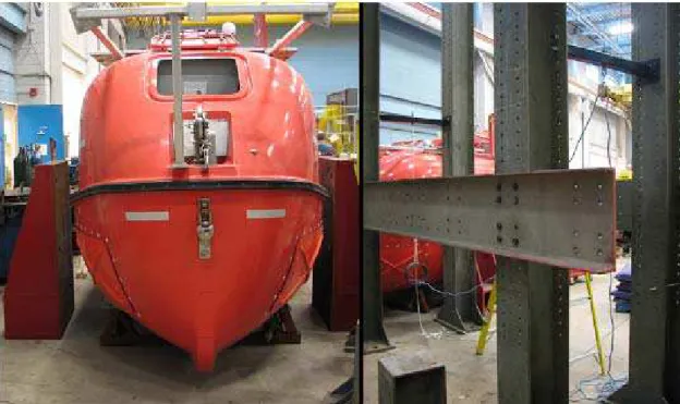
List of Figures Figure 1: Supports and Frame……….………2
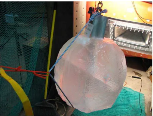
Figure 2: Specimen Harness………....4
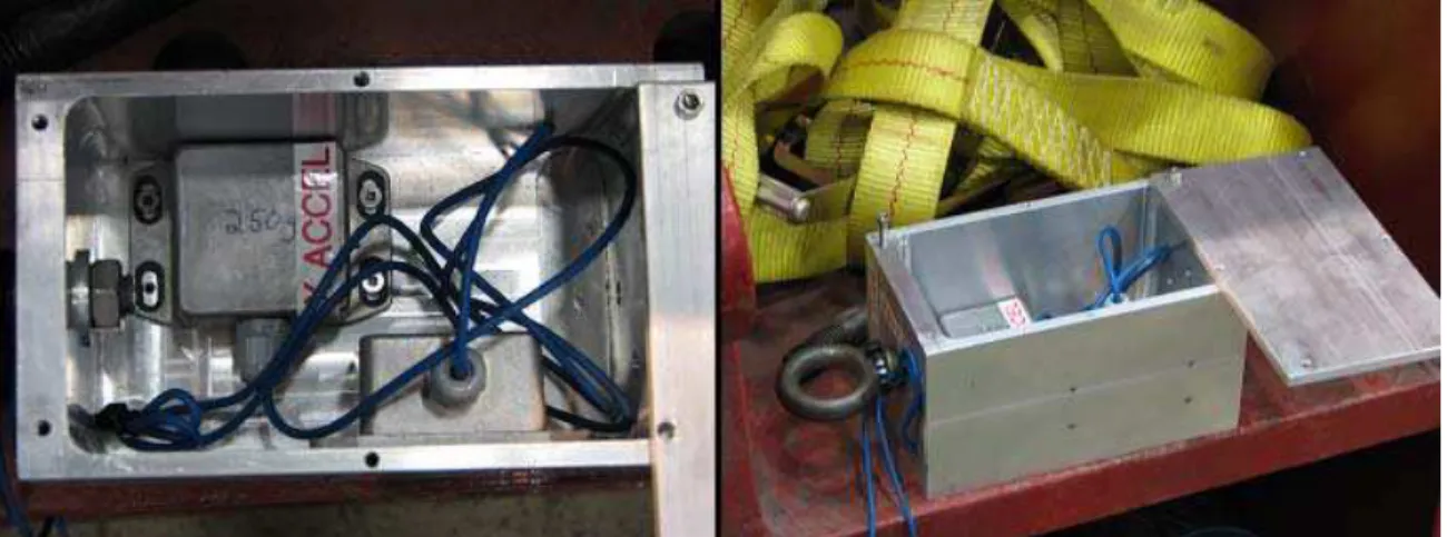
Figure 3: Accelerometers………...……….5
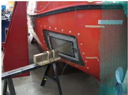
Figure 4: 0.5-inch LVDT……….6
Figure 5: High-Speed Camera Calibrations……….8
Figure 6: Specimen Before and After Impact………...9
Figure 7: Mounting the Accelerometers……….….10
Figure 8: Measuring the Angle……….11
Figure 9: Acceleration vs. Time……….……….15
Figure 10: Force vs. Time (1 tonne)……….………....15
1.0 Introduction
From March 17th to March 23rd 2009 the Institute for Ocean Technology (IOT) conducted a series of experiments on a modified 20-person Totally Enclosed Motor Propelled Survival Craft (TEMPSC) lifeboat in the MUN Structures Lab. Its modifications included the addition of port and starboard acrylic impact panels to the hull, mounted on force dynamometers. To accommodate the panels and force dynamometers, two sea chests were manufactures and incorporated in to the hull structure.
The experiments involved suspending an ice sphere from a rope as a pendulum. The sphere was then set at a specified angle, and allowed to freefall in the pendulum’s natural arc, impacting the panel. This process was repeated at various angles and in various impact areas on the panel in order to collect a variety of data from instrumentation such as accelerometers, LVDT’s, load cells, and cameras.
The tests were carried out for various objectives to be utilized by IOT researchers and by Master's degree student Allison Kennedy. The project team at IOT was interested in:
1. Verifying the accuracy of the dynamometer (dyno).
2. Finding the optimal dyno filter setting for upcoming sea trials..
3. Ensuring that the modified hull structure was stable due to the addition of the acrylic panels
For Allison Kennedy, the objective was to:
4. Determine the coefficient of restitution of the ice and hull interaction 5. Estimate the ice crushing energy vs. the impact energy.
These final two objectives are to be used in a mathematical model that is being prepared to simulate the effects of impacts on the lifeboat with ice, as they interact in the field.
2.0 Experimental Apparatus 2.1 Facilities
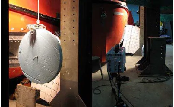
All of the testing was carried out in the MUN Structures Lab. The Lifeboat was braced with a strap over the bow and secured to wedge-shaped supports on both sides, and shown on the left in Figure 1 and at point 1 in Appendix A. The frame for suspending the pendulum was constructed using four 5.0 m x 0.30 m I-beams, and braced with rails that spanned the distance between sets of two beams. This frame is shown on the right in Figure 1, and at point 2 in Appendix A.
2.2 Layout and Equipment
The frame was placed perpendicular to the panel being tested to ensure that the ice specimen would impact directly without sliding or scraping along the panel. The majority of the tests were conducted on the port side of the boat, deemed the “working” side with the starboard panel as the “non-working” side. This is a reference to the equipment inside the panel as the force dynamometer (dyno) on the starboard side was not in operation during the tests.
The bracing over the bow as well as twelve sand bags weighing 50 lbs. each helped to prevent the boat from moving on impact. For convenience, the lifeboat was placed in a cradle rather than remaining in its trailer, also contributing to its grounding. In using the cradle however, the lifeboat was lowered requiring an alteration in the original measurements for the cross bar that suspended the pendulum. Two of these cross bars were used at approximately the same height between the sets of two I-beams. These bars were designed in AutoCAD and were fabricated at IOT for this experiment. They are seen at point 3 in Appendix A, suspending the ice specimen and supporting the winch that is used to hoist the specimen to the desired release angles.
During the planning stage of the experiment, a pulley system was included to hoist the specimen as well as a quick release. After the first day of testing however, it was decided that the pulley system was too physically strenuous in that a person was to hoist a 200 lb. specimen up to the desired release angle using only a rope and pulley. There were also concerns that the quick release system would require a significant force to release which could potentially skew the path of the pendulum, resulting in an off target impact. As a result of these concerns, a motorized winch was used to raise the pendulum, and a line was cut as the release. The line can be seen in orange in Figure 2, which includes the harness that was used to hold the specimen. Since various angles were used to impact, it would have been difficult to pull the specimen from the same point while also allowing the pendulum to swing in its natural arc. The harness used allowed the specimen to be pulled from various points depending on the angle
required, while allowing the pendulum rope to remain taut, swinging naturally when released.
2.2.1 Instrumentation
The dynamometer (dyno) inside each panel is made up of 6 U2B Force Transducers (load cells). These load cells are connected with flex links, allowing the movement that is needed for the dyno to work properly. There are three load cells with a 1 tonne capacity, and three with a 5 tonne capacity. The
specifications including images and dimensions for these load cells can be found in Appendix B. During the experiment, only one panel was working, therefore all the force data was collected from the port panel.
Inside the lifeboat there is a MotionPakTM, which is an inertial sensing system that measures the accelerations in the x, y and z direction of the lifeboat as it was impacted. It is located at point 4 in Appendix A, and further descriptions can be found in Appendix C.
Mounted to each ice specimen during impact were two Surface Mount Micromachined Accelerometers that are shown in Figure 3 and have data sheets presented in Appendix D. These accelerometers measured the acceleration of the pendulum in the x and y directions from release to impact.
Figure 3: Accelerometers
There were two GCD-SE Series Precision Gage Heads (LVDT’s) used during testing to measure the movement of the boat during an impact. The specifications for these LVDT’s are located in Appendix E. The 0.25-inch LVDT was placed inside the lifeboat against the sea chest holding the panel that was
being tested in order to record how much the panel moved during impact. The 0.5-inch LVDT was placed outside the lifeboat against the opposite panel, to record the movement of the panel that was not being impacted. The 0.25 and 0.5 inch LVDT’s are located at points 5 and 6 respectively in Appendix A, and the 0.5-inch LVDT can be seen outside the lifeboat in Figure 4 below.
Figure 4: 0.5-inch LVDT
A high-speed camera was used to record every impact in order to find the impact speed from the video. Its position can be seen at point 7 in Appendix A. The camera used was a Photron Ultima APX-RS and in conjunction with the camera, an automatic trigger function was used for the first half of the testing. Due to lighting and lack of contrast, the automatic trigger began to trigger late in the swing of the pendulum, causing the camera to begin recording just as the specimen impacted, or in some cases miss the impact entirely. A manual trigger was then used to capture the impact for approximately half of the testing. A Canon hand-held PowerShot S2 IS was used during the experiment to document all aspects of the procedure. The Canon was used to take pictures of the set up and decommission, as well as specific parts of the impacts. As well, it was used to record videos of every impact. There was also a Defender Security camera placed on one of the beams (positioned at point 8 in Appendix A) to record each
impact, as well as a Defender Security black & white, weatherproof bullet type camera placed inside both panels, looking out of the lifeboat.
A scale was made available to weigh each ice specimen before any impact had occurred. Each specimen was weighed in pounds before the impacts began and again when it was either deemed too damaged to be used further, or when the specimen itself shattered. It can be seen at point 9 in Appendix A.
Every instrument with the exception of the high-speed camera, Canon hand-held camera, and the scale were wired together, resulting in 16 data
logging channels. These channels were operated using a remote unit, which was designed and built at IOT along with its corresponding software. The software used to log the data from the load cells and accelerometers, iLogger, was also developed at IOT. This software was used in conjunction with an IOtech
DaqBoard 3000, an analog to digital unit that converts the analog voltage reading given by the instruments into a digital numerical reading. The data was recorded onto a laptop inside the lifeboat, which was connected via a network cable to a laptop outside the boat for operators located at point 10 in Appendix A. The video from the cameras inside the panels along with the security camera outside the lifeboat was stored on Secure Digital (SD) cards. These cards varied from class 2 to class 6 specifications, meaning that the rate of transfer of the videos was slow in the class 2 while the class 6 was a higher speed. This meant that it took substantial time to transfer the videos, temporarily halting the experiment
3.0 Methodology 3.1 Calibrations
Before the high-speed camera could be used, it needed to be calibrated to suit our purposes. The foam cylinder seen in Figure 5 was used to aid in
adjusting the camera settings.
Figure 5: High-Speed Camera Calibrations
The calibrations performed included adjusting the frame rate (fps) and the resolution (pixels) in the camera settings. Since the automatic trigger was initiall used to record the videos, MiDAS Player was used with the camera. However, when the manual trig
y
ger was introduced, the program was switched to Photron ASTC
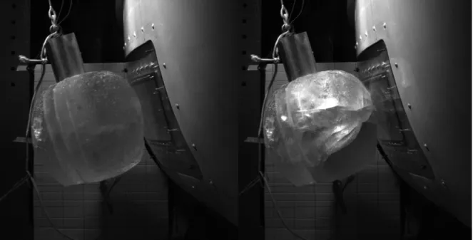
ample of the quality of video recorded is seen in Figure 6 which clearly shows a
F AM viewer.
It was decided that a frame rate of 3,000 frames per second (fps) was unnecessary for the purposes of these trials; therefore a rate of 1,000 fps was used. During test set 4, which will be elaborated upon in the next section, it was decided that a lower frame rate of 500 fps was more appropriate. The resolution of the recording was 1024 x 1024-pixels throughout the experiment. An ex
specimen just before and just after an impact. The videos were saved as a series of .jpeg images due to the size that the files would be in any other form.
3.2 Procedure
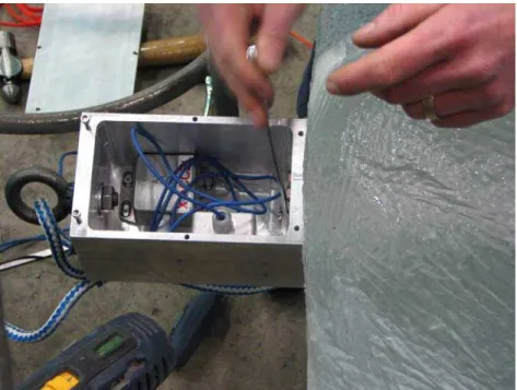
A total of 33 tests were performed with 9 ice specimens. Specimens were brought to the Lab as needed, in order to maintain a similar temperature between specimens. A hole was then drilled into the specimen, and a probe was inserted in order to measure the temperature approximately 3 inches below the surface of the ice. It was then weighed (in pounds) and brought to the center of the frame to attach the accelerometer box.
Figure 7: Mounting the Accelerometers
After the accelerometers were attached (Figure 7), the specimen was raised and attached to a rope, with the length of the pendulum 2.0 m from the center of the specimen to the bottom of the eye hook attached to the cross bar. The specimen was then raised to the desired angle, as specified by the test set. There were a total of four test sets that were completed during this experiment: Test set one- impacts in the center of the working side, repeated at 20°. This test was performed while adjusting the filter, to find the optimal setting. It was found to be 8,000 Hz for the load cells and 800 Hz for the other instruments. The sampling rate for the data was 50,000 Hz. These rates remained constant throughout the experiment.
Test set two- impacts in the centre of the working side at various release angles. This was done to create an impact force vs. dyno reading curve in order to verify the dyno.
Test set three- impacts at critical points forward and aft of centre on the panel. These impacts were directly on the load cells, hence why these points are the critical points on the panel. This set was completed to verify an impact force vs. dyno reading curve at these points.
Test set four- impacts in the centre of the non-working (dummy) side. This was performed in order to see the reading of an impact on the opposite side, that is, the effect of an impact on the starboard side was recorded on the port side.
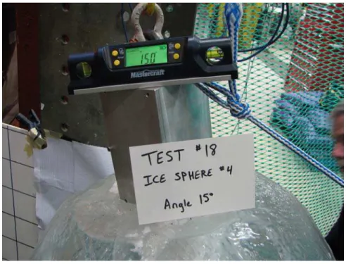
After the specimen was raised to the specified angle, a picture was taken to record that the angle was correct as shown in Figure 8. The temperature of the specimen was taken again just prior to release.
Figure 8: Measuring the Angle
Ensuring that all instruments were logging and that the team was ready to begin, a countdown was started and the specimen was released. It was allowed to swing in the pendulum’s natural arc into the panel then restrained after impact
to avoid the specimen hitting the panel a second or third time. Multiple impacts would disrupt the data, resulting in an uncertainty in the analysis.
The panel was then inspected visually, and the team verified whether or not the impact had been recorded by checking their data logs/recordings. If the specimen shattered, the largest pieces were weighed to compare with the initial weight. Differences were accounted for with the melting of the ice and the crushed ice that was produced on impact. If the specimen was intact, it was rotated to a surface free of previous impacts. Any debris on the test site was cleaned up, and the specimen was set up to impact again. This procedure can be seen in checklist form in Appendix F. An overview of the test matrix listing the tests, test set, specimen used, impact area and angle is located in Appendix G. It can be seen in this test matrix that test set two was completed twice. This was due to the MotionPakTM recording accelerations that exceeded its limits. This may have been due to the rigidity of the surface beneath the MotionPakTM, therefore foam was added to the surface and the tests were completed again in order to validate the first set of readings. The full test log is located in Appendix H, which lists all recorded values, setbacks and general observations for all impacts performed.
4.0 Results
With a total of 33 tests and 9 specimens, there was over 36 GB of information collected including raw data, videos and pictures. Due to this large amount of data and the time constraints on the work term, only one test will be analyzed as a representation of the results.
The test that has been chosen is Test 19, Specimen 4. Its initial weight was 208 lbs, and it was released aft of center at 20° as part of Test Set 3. More information about this test can be found in Appendix H.
As previously stated, the dyno measures the force of impact, and the accelerometers measure the acceleration of the specimen. This information therefore, can be used as a simple verification of the dyno if Newton’s second law is applied to the data. The law states: “The acceleration of an object is directly proportional to the net force acting on it and inversely proportional to its mass.” (Serway & Jewitt, 2006). This law is written as:
(Equation 1)
However, it is most commonly seen in its mathematical form,
(Equation 2)
This makes the relationship equality rather than proportionality, which is a valid alteration only if the speed of the given specimen is recognized as much less than the speed of light (Serway & Jewitt, 2006). For the purposes of this example, Equation 2 will be rearranged to suit our data. That is, given that the weight of each specimen was recorded before any impacts had taken place, the weight can be calculated using the data collected from the dynos and
accelerometers.
The data files logged from the load cells were saved as Microsoft Excel Comma Separated Values File (.csv files). These files were far too large to be loaded and analyzed in Microsoft Excel; therefore Igor Pro 6.0 was used for the
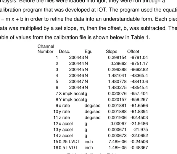
analysis. Before the files were loaded into Igor, they were run through a
calibration program that was developed at IOT. The program used the equation y = m x + b in order to refine the data into an understandable form. Each piece of data was multiplied by a set slope, m, then the offset, b, was subtracted. The table of values from the calibration file is shown below in Table 1.
Channel
Number Desc. Egu Slope Offset 1 200443 N 0.298154 -9791.04 2 200444 N 0.29662 -9751.17 3 200445 N 0.296388 -9692.82 4 200446 N 1.481041 -48365.4 5 200447 N 1.480778 -48413.6 6 200449 N 1.483275 -48545.4 7 X impk accel g 0.020076 -657.404 8 Y impk accel g 0.020157 -659.267 9 x rate deg/sec 0.001881 -61.6566 10 y rate deg/sec 0.001888 -61.8394 11 z rate deg/sec 0.001906 -62.4503 12 x accel g 0.00067 -21.9486 13 y accel g 0.000671 -21.975 14 z accel g 0.000673 -22.0652 15 0.25 LVDT inch 7.48E-06 -0.24506 16 0.5 LVDT inch 1.48E-05 -0.48367
Table 1: Calibration Table
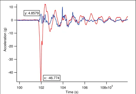
The following graphs are plots from Igor to illustrate the data. Figure 9 shows the x and y accelerations that were recorded in the accelerometers mounted on the specimen. The accelerations are recorded in g’s, and therefore needed to be converted into a more standardized unit (m/s2).
-40 -30 -20 -10 0 10 A ccel e ra ti o n (g ) 108x103 106 104 102 100 Time (s) x: -46.774 y: 4.8579
Figure 9: Acceleration vs. Time
Shown in Figures 10 and 11 are the forces recorded in Newtons by the three 1 tonne load cells, and the three 5 tonne load cells, respectively.
8000 6000 4000 2000 0 -2000 -4000 -6000 Force ( N ) 115x103 110 105 100 Time (s) 443: 7390.8 444: -7163.2 445: -5543.8
20x103 15 10 5 0 -5 -10 Fo rce (N) 108x103 106 104 102 100 Time (s) 446: 11696 447: -12763 449: 21354 `
Figure 11: Force vs. Time (5 tonne)
In the 3 previous figures, the maximum or minimum value is noted which indicates the moment of impact. These peaks were inserted into an Excel spreadsheet along with the offset from zero that is also found in each graph. These offsets were subtracted from the peaks, yielding the absolute value. The vector sum was then taken of the forces and accelerations; the peaks were squared, the 1 tonne loads, 5 tonne loads and x and y accelerations were summed then the square root was taken. The forces from the 1 tonne and 5 tonne loads were summed to create total force. The total acceleration was multiplied by 9.80665 to convert the units from g’s to m/s2. This process can be followed in Table 2, an excerpt from the spreadsheet.
Load (N) peak offset subtract square sum
square
root Total Force 1t 443 7390.8 589.574 6801.226 46256675.1 131456556 11465.451 39493.4603 N 444 -7163.2 85.5157 -7248.7157 52543879.3 445 -5543.8 170.743 -5714.543 32656001.7 5t 446 11696 -600.129 12296.129 151194788.4 785569329 28028.01 447 -12763 304.794 -13067.794 170767240 449 21354 -177.542 21531.542 463607300.9 Accel. (g) Acceleration x -46.774 0.143676 -46.917676 2201.268321 2226.5084 47.185892 462.735527 m/s2 y 4.8579 -0.16605 5.02395 25.2400736 m = 85.347802 kg Actual Weight = 208 lbs = 188.1597 lbs Percent error = 9.54% Table 2: Sample Calculation
With the acceleration in m/s2, equation 2 could now be utilized, but rearranged into Equation 3 below:
(Equation 3)
This yielded a mass of 85.3748 in kilograms since a Newton is defined as 1 kg m/ s2, and therefore dividing it by m/s2 leaves only kg. This unit is not
comparable to the measured weight of the specimen, and was therefore
multiplied by a factor of 2.20462262 to convert kg to lbs. This conversion showed a weight of 188.1597, which is approximately 20 pounds lower than the
measured weight of the specimen. Then, the percent error was calculated using the formula 1-(calculated/actual), giving an error of 9.54%.
This calculation can be used as a verification of the readings from the dyno in the panel, since the calculated value was of an acceptable percent error from the measured value. Causes for the error could stem from noise in the dyno, environmental conditions, or inaccuracy either in the scale used to weigh the specimen initially or in the accelerometers.
5.0 Conclusions
In reflecting on the initial objectives of the experiment, the following conclusions can be drawn.
1. It can be said that the dyno registers accurate readings with the results of the calculations seen in Section 4.0. The value calculated was within an acceptable tolerance of error.
2. The optimal filter settings were found to be 8,000 Hz for the load cells located in the dyno, and 800 Hz for all other instruments. This was used in conjunction with an acceptable sampling rate found at 50,000 Hz.
3. The hull structure appears to be stable, as no visible damage was done to the lifeboat. Further examination will be done on the panels however, to search for cracks, scratches or other structural deficiencies that would not be visible by the naked eye.
4. & 5. The experiment was successful in that there was enough data collected to facilitate the calculation of the coefficient of restitution of the ice and hull interaction and to find an estimate for the ice crushing energy vs. the impact energy. However, the majority of this data has not yet been analyzed and therefore the value of these quantities cannot be
6.0 Recommendations
The following recommendations are made in order to improve the
performance and progress of experimental analysis. It is suggested that these recommendations are followed if this experiment is to be repeated in the future.
1. While an automatic trigger function for the high-speed camera is very convenient, it was found to be unreliable. There were numerous occasions when the camera did not trigger, causing the video to miss the impact. A manual trigger was then used which considerably improved the content of the video. The trigger should be used for the entirety of the experiment to avoid missing significant video.
2. SD cards were used to store video from the cameras as mentioned earlier in the report. These cards were slow in transferring the data, especially as they filled. Class 6 cards should be used for all data storage as they are faster, meaning less time spent waiting for files to transfer.
3. The boat was initially scheduled to move to the MUN Lab on Monday, March 9th, but was delayed a week. When the panels were placed into the boat that morning, it was discovered that one did not fit into its place in the hull. This caused a weeks delay since the panel had to be altered to fit, and the boat was moved to the lab later that week testing began the following week. With time restraints on the test period, all parties involved should be certain that the equipment is ready to go for the specified date.
7.0 Works Cited
Raymond A. Serway & John W. Jewett (2006) Principles of Physics. Canada: Brooks/Cole – Thomson Learning