TROPOSPHERE DURING THE 20TH CENTURY
S. BR ¨ONNIMANN1,∗, T. EWEN1, T. GRIESSER1and R. JENNE2 1Institute for Atmospheric and Climate Science, ETH Z¨urich, Universit¨atstrasse 16, CH-8092
Z¨urich, Switzerland
2National Center for Atmospheric Research (NCAR), Boulder, CO, USA (∗Author for Correspondence, E-mail: stefan.broennimann@env.ethz.ch)
(Received 31 August 2005; Accepted in final form 21 December 2005)
Abstract. Studies based on data from the past 25–45 years show that irradiance changes related to the 11-yr solar cycle affect the circulation of the upper troposphere in the subtropics and midlatitudes. The signal has been interpreted as a northward displacement of the subtropical jet and the Ferrel cell with increasing solar irradiance. In model studies on the 11-yr solar signal this could be related to a weakening and at the same time broadening of the Hadley circulation initiated by stratospheric ozone anomalies. Other studies, focusing on the direct thermal effect at the Earth’s surface on multidecadal scales, suggest a strengthening of the Hadley circulation induced by an increased equator-to-pole temperature gradient. In this paper we analyse the solar signal in the upper troposphere since 1922, using statistical reconstructions based on historical upper-air data. This allows us to address the multidecadal variability of solar irradiance, which was supposedly large in the first part of the 20th century. Using a simple regression model we find a consistent signal on the 11-yr time scale which fits well with studies based on later data. We also find a significant multidecadal signal that is similar to the 11-yr signal, but somewhat stronger. We interpret this signal as a poleward shift of the subtropical jet and the Ferrel cell. Comparing the magnitude of the two signals could provide important information on the feedback mechanisms involved in the solar climate relationship with respect to the Hadley and Ferrel circulations. However, in view of the uncertainty in the solar irradiance reconstructions, such interpretations are not currently possible.
Keywords: solar variability, Hadley cell, Ferrel cell, multidecadal variability
1. Introduction
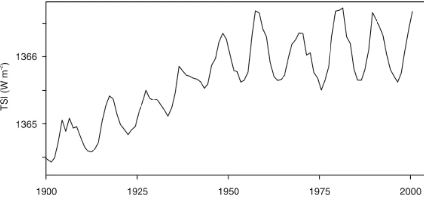
Solar irradiance changes have been found to influence global surface climate on various time scales (e.g., Bond et al., 2001; Haigh, 2003; Lohmann et al., 2004; see also Rind, 2002), including multidecadal variability. One of the key periods in this respect is the first half of the 20th century. According to reconstructions, total solar irradiance (TSI) increased by around 0.8 to 1.5 W/m2 during this
pe-riod (see Figure 1) and global surface air temperatures increased by about 0.5◦C, which is comparable in magnitude to the warming since the 1970s (Jones et al., 1999). To what extent the warming was caused by solar variability is debated. Model simulations suggest that both anthropogenic and natural influences con-tributed (Schlesinger and Andronova, 2004; Stott et al., 2001; Ingram, 2006), but Space Science Reviews (2006) 125: 305–317
Figure 1. Reconstruction of solar radiation by Lean (2004).
the warming is still underestimated by many simulations and the question is not yet solved (e.g., Meehl et al., 2003).
While the solar impact on climate is increasingly well accepted in the scientific community, the mechanisms that produce it are not. Some of the detected influences energetically do not match well with the supposed forcing, feedbacks have to be involved, and the dynamics of the whole ocean-atmosphere system needs to be considered (see Rind, 2002; Haigh, 2003). Stratospheric ozone seems to play an important role for the stratospheric signal, which then can be communicated to the troposphere, but the details of this mechanism are not clear (e.g., Balachandran et al., 1999; Shindell et al., 1999; see also contributions by Gray et al., and Haigh and Blackburn in this issue). Solar variability has also been suggested to influence climate via a cloud feedback (Svensmark and Friis-Christensen, 1997; Tinsley and Yu, 2004), but again the mechanisms are debated.
One of the key questions relates to the response of the Hadley and Ferrel circula-tions. An 11-yr solar signal has been found in zonal mean geopotential height (GPH) and temperature at midlatitudes in the free troposphere at around 30◦–60◦N (e.g., Labitzke and van Loon, 1997; van Loon and Shea, 1999; Labitzke, 2003; Haigh, 2003; Gleisner and Thejll, 2003; Crooks and Gray, 2005), with higher tempera-tures and GPH accompanying higher irradiance. The signal has been interpreted as a northward displacement of the subtropical jet and the Ferrel cell. In a series of model studies on the 11-yr solar signal considering both irradiance changes and ozone changes (Haigh, 1999; Larkin et al., 2000), this signal could be related to a weakening and at the same time broadening of the Hadley circulation initiated by stratospheric ozone anomalies. Other studies focusing on the direct thermal effect at the Earth’s surface on multidecadal scales (using long integrations with models that do not include ozone changes), suggest a strengthening of the Hadley circulation due to a solar-induced change in tropical temperature gradients (Meehl et al., 2003, 2004; van Loon et al., 2004). According to this mechanism, the thermal solar signal is strongest in subtropical cloud free areas and affects the Hadley cell via moisture
transport, precipitation, and latent heat release (and a feedback on subtropical cloud cover). This is consistent with observations that point to an increase in strength of the Hadley circulation during the past century, but the uncertainty in the data is very large (Evans and Kaplan, 2004).
It would be desirable to find a framework that allows for an overarching dis-cussion of solar-climate effects on the Hadley and Ferrel circulations in the 20th century. However, many problems remain to be solved. This concerns not only the poorly known feedbacks of the climate system, but also the actual forcing mecha-nisms, which might be different at the two time scales (e.g., due to different spectral characteristics of the irradiance change).
One important gap is that the studies on the solar signal in the upper troposphere are based on the last two to four solar cycles only, which were characterised by a large amplitude of the 11-yr cycle, but no or little low-frequency variability (Figure 1). It would thus be very interesting to repeat the studies for the first part of the 20th century, when TSI (according to Lean, 2004) increased substantially. Up to now, data from the upper troposphere that would be needed for such a study have not yet been available. During the past few years we have compiled, digitised, and re-evaluated a large amount of global upper-air data reaching back to around 1920. The data originate from radiosonde, pilot balloon, aircraft, and kite ascents performed in many parts of the world. These data are used in a statistical reconstruction approach to derive zonal mean GPH and temperature up to the 200 hPa level. We focus on the latitude band 30◦–60◦N, where we expect the signal to be strongest. Then we extract the solar signal from the zonal mean series using a simple regression approach and try to answer the following question: Is there a multidecadal signal in the upper troposphere during the 20th century, and if so, how does it compare with the 11-yr signal?
2. Data and Methods
We used monthly historical upper-level data that have been re-evaluated in recent years (Br¨onnimann et al., 2005b). These data sets include the UA39 44 upper-air data for the extratropical northern hemisphere, 1939–1944 (Br¨onnimann, 2003), with recent updates (Version 1.1, S DCRM), consisting of radiosonde and aircraft observations of temperature and GPH on pressure levels. In addition, earlier U.S. data from kites and aircraft were taken from the Monthly Weather Review, 1922– 1938, consisting mainly of temperature on geometric altitude levels up to 5 km from kites and aircraft. Radiosonde data on pressure levels from the IGRA data set (1945–1947, Durre et al., 2005) and from the Finnish station Ilmala, 1942–1947, were also used (Br¨onnimann et al., 2005a) as well as upper level wind (on geometric altitude levels) from selected stations, 1922–1947 (NCAR, TD52 an TD53 data sets, see http://dss.ucar.edu/docs/papers-scanned/papers.html, documents RJ0167, RJ0168).
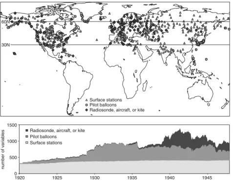
In total, 253 upper-air stations were used (Figure 2). Note, however, that at each station the record covers only part of the period. The bottom part of Figure 2 shows the number of available predictor values per month during the historical period (1922–1947). The data availability is best for the War time, but some upper-air data are available back to 1922. The data clearly do not suffice to directly calculate reliable zonal averages for different levels, which is also made impossible by the different vertical coordinates (pressure, altitude). Hence, we used a statistical reconstruction approach to obtain the zonal means.
The upper-level data were supplemented with data from the Earth’s surface, which also contribute information to the statistical reconstruction approach. For this purpose we used a set of 387 surface air temperature records from the NASA-GISS database (Hansen et al., 1999). The stations are chosen to cover the northern extratropics. If possible, mountain sites were chosen (see Figure 2, top). In addition, we used gridded sea-level pressure (SLP) (HadSLP2, Allan and Ansell, 2005) and sea-surface tempertaure (SST) (ERSST V2, Smith and Reynolds, 2004) data. These data were included in the form of latitude-weighted principal component (PC) time series of the monthly anomaly fields north of 20◦N (calculated for 1900– 2003.) For SLP and SST, we retained 20 and 32 PCs, respectively, corresponding to approximately 95 and 90% of the total variance.
Figure 2. Top: Map of upper-air and surface stations used for the reconstruction. Bottom: Number
In order to reconstruct zonal mean temperature and geopotential height from the historical upper-level station data, statistical models need to be calibrated in a period for which both the station data and the zonal means are available and have no or only few gaps. We used the 1948–2003 period, where the zonal means can be calculated from NCEP/NCAR reanalysis data (Kistler et al., 2001). In many cases, upper-level station data are not available for the same locations, or they have long gaps. Therefore, we decided to use NCEP/NCAR reanalysis data, interpolated to the station location and levels, to supplement the historical upper-level data in all cases. However, reanalysis data are a model product which is somewhat different from observations. Additional errors arise from the fact that historical data have a lower quality than more recent observations and from the interpolation procedure. To account for these errors, we randomly perturbed the supplemented predictors by a normally distributed noise. The error (standard deviation of the noise) was estimated based on our quality assessment (see references above), which itself was based on NCEP/NCAR reanalysis as a reference.
Gaps in the surface station data are short. They were filled with corresponding NCEP/NCAR reanalysis data at 925 hPa after the standardising procedure (see below). The PC time series for the SLP and SST fields have no gaps. In this way, a calibration data set can be constructed that has no missing values in the 1948– 2003 period. All predictor data series were then expressed as anomalies from the 1961–1990 mean annual cycle and were standardised.
The statistical model used is a simple principal component regression. Due to missing values prior to 1948, each month in the historical period has a different combination of available variables and therefore reconstructions were performed independently for each month from 1922 to 1947. A three-calendar-months moving window was used for calibration, e.g., to form a reconstruction model for January 1922 we used all Decembers, Januaries, and Februaries in the calibration period. First, for each time step the available variables were weighted as follows. We attributed 25% of the weight to the surface and the rest to the upper-level data. Within the surface data, half of the weight was attributed to the SLP PCs and one fourth to station temperature and one fourth to the SST PCs. Within the SLP PCs and SST PCs, the weight was split according to their correlation with SLP or surface (land and marine) air temperature averaged from 30◦–60◦N, respectively. Within the upper-level data, half of the weight was attributed to the pilot balloon data, half of the weight to the upper-level temperature or geopotential height data. This weighting scheme gave much better results than using no weighting at all.
After the weighting, a principal component analysis was performed on all avail-able predictor variavail-ables in the calibration period in order to reduce the number of variables. Thereby the amount of variance retained was varied between 70 and 98% and the optimum fraction (according to the validation experiments, see below) was chosen for each month.
The reconstructions were validated using two split-sample validation experi-ments, i.e., the calibration period was split and one part was used for calibrating the
model, the other for validating the model. In the first experiment we used 1948–1966 for validation, in the second 1985–2003. Out of the many different reconstruction models (varying amount of retained variance), we chose for each time step (one month) the one that had the highest reduction of error (RE, see Cook et al., 1994), averaged from both validation experiments. Values of RE can be between −∞ and 1 (perfect reconstructions). RE> 0 determined in an independent period is normally considered an indication that the model has predictive skill.
3. Results 3.1. RECONSTRUCTIONS
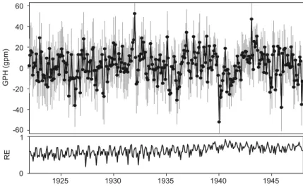
Figure 3 shows the reconstructed 300 hPa GPH anomalies as an example. The recon-structions capture variability from the month-to-month to the interannual scale. The anomalously high value in January 1932 is robust with respect to the amount of vari-ance retained and the weighting used. The strongly negative values in 1940–1941 coincide with a global climate anomaly related to an El Ni˜no event (Br¨onnimann et al., 2004). There is a slight positive bias of 3.8 gpm which, however, does not vary much with the amount of retained variance and only slightly with season. The RE statistics (lower panel) shows a clear annual cycle. Reconstructions are good in late winter, whereas they are less reliable in May. Also, the RE changes with time due to the change in the predictor variables. During the War, a large amount of upper-air data is available and the reconstructions are much better. Over all, the reconstructions can be considered as relatively good, with RE values mostly in the
Figure 3. Top: Reconstructed monthly 300 hPa GPH from 1922 to 1947 with 95% confidence intervals
calculated from the two split-sample validation experiments. Bottom: RE from the two split-sample validation experiments.
range of 0.6 to 0.8 (higher than 0.5 in 83% of the cases). This is sufficient for the following analyses. To account for the possible bias, the regression analyses presented in the next section includes a step function in 1948.
3.2. REGRESSION MODEL
The reconstructed zonal means were merged with NCEP/NCAR data after 1948, yielding 82-year long time series. All analyses were performed for both tempera-ture and GPH, for summer (Jun− Aug) means and for the annual means. In the following we focus on annual mean values of GPH for which we expect a more robust signal and better reconstruction quality (results were similar for the other analyses). The time series were related to solar variability in a regression approach, similar as in Haigh (2003), Crooks and Gray (2005), and other studies. As a mea-sure for solar variability we used the TSI reconstructions by Lean (2004), shown in Figure 1, which we updated to 2003 with satellite data from PMOD/WRC (Davos, Switzerland). In addition, we accounted for stratospheric aerosols in the Northern Hemisphere (Sato et al., 1993) as well as the El Ni˜no index NINO3.4 (assuming that El Ni˜no/Southern Oscillation is independent from the solar signal). Both variables were used with a 6 month lead time, which is considered a typical response time of extratropical circulation to these forcings (results are not sensitive to the choice of the lead). Other studies (e.g., Crooks and Gray, 2005) also include the North Atlantic Oscillation (NAO) or other circulation variability modes as explanatory variables. However, several authors (e.g., Shindell et al., 2001) suggest that the mechanism linking solar variability to tropospheric circulation might include the NAO or Northern Annular Mode. Therefore, we repeated all analyses with and without using the NAO (SLP difference between 37.73◦N, 23.7◦W and 64.13◦N, 21.9◦W from HadSLP2 data) and PNA (reconstructed exactly as described above using a subset of the data, manuscript in preparation) as explanatory variables in our analysis.
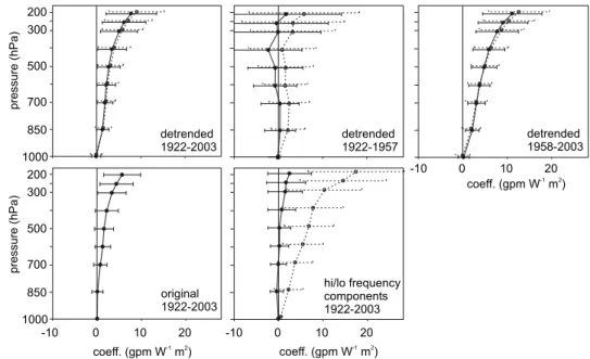
In a first step we focused on the 11-yr time scale and subtracted from each variable the low frequency variability in the form of a 4th order polynomial func-tion in time. We then performed a multi-linear regression in three time periods: 1922–1957, 1958–2003, and 1922–2003. The coefficients are shown in Figure 4 (top, note that for display purposes, 90% confidence intervals are used). The coeffi-cients for the 1958–2003 agree well with previous studies. No signal at all is found at the surface. With increasing altitude, the signal becomes strongly positive and highly significant. In the 1922–1957 period, confidence intervals are much larger, especially in the upper troposphere. This is expected to some extent. The signal (amplitude of the 11-yr cycle) is only about half as strong in the earlier period. At the same time the uncertainty of the reconstructions, especially at higher levels, also contributes. When analysing the whole period (1922–2003, Figure 4 top left), we find again significantly positive coefficients. The coefficients do not change much
Figure 4. Top: Coefficient (90% confidence intervals) for TSI from multiple regression models of the
annual mean GPH (30◦–60◦N average) using detrended data for 1922–2003 (left), 1922–1957 (middle) and 1958–2003 (right) with only TSI, NINO3.4 and volcanic aerosols as explanatory variables (dashed lines), or TSI, NINO3.4, volcanic aerosols, NAO, and PNA (solid lines). Bottom: Same for models which are based on the non-detrended data (1922–2003), but which include further explanatory variables in addition to TSI, NINO3.4, volcanic aerosols, NAO and PNA (left). In the middle figure TSI is split into an 11-yr (solid) and a background component (dashed).
when including NAO and PNA as explanatory variables. The confidence intervals decrease slightly. However, the overall model statistics (not shown) improve sub-stantially. In all, we have no statistical evidence to assume that the relation between solar variability on the 11-yr scale and atmospheric circulation is non-stationary, but the signal is clearly less obvious in the earlier period.
The first part of the record is mainly interesting with respect to multidecadal variability. Therefore, in a second analysis we used the whole period but did not detrend the data. Instead, we included a number of other terms in the regression model that could possibly explain low-frequency variability in our target variables. In addition to the volcanic forcing and El Ni˜no used above, we included greenhouse gas and tropospheric aerosol forcing from Crowley (2000). The two series were updated to 2003 using a linear relation to observed annual mean CO2concentrations
(provided by CDIAC via their website http://cdiac.esd.ornl.gov/) or a second order polynomial in time, respectively, calibrated in the 1959–1998 period. In addition, we introduced two step functions to account for possible inhomogeneities in the data: in 1948 (merging of reconstructions with NCEP/NCAR reanalysis) and in 1979 (main start of satellite data used in NCEP/NCAR). Again, including NAO and PNA has
a relatively small effect on the results, but general model statistics improve greatly, with explained variances between 54 and 68% (this is surprisingly high given the fact that a large part of the record is reconstructed). Figure 4 (bottom left) shows the coefficients found for TSI in a model that includes NAO/PNA. They are similar, though somewhat weaker, to those found on the 11-yr time scale in the top left panel. To further analyse the effect of the time scale, we used the same regression model, but additively split TSI into an 11-year and a low-frequency component (as given in Lean, 2004). Coefficients for the two components are given in Figure 4 (bottom right). For the 11-yr component we expect similar coefficients as in the other analyses, but find smaller, insignificant coefficients. On the other hand, the coefficients for the multidecadal scale are larger, and they are significantly different from zero at higher levels.
The different sets of coefficients are just within each others 90% confidence intervals. This means that from our analysis we have some weak indications, but no firm evidence to assume that the solar signal in the upper troposheric circulation is different in strength on the 11-yr scale than on the multidecadal scale.
4. Discussion
Up to now the effect of solar variability on upper tropospheric GPH was only studied effectively for the 11-yr cycle. Our analysis reveals a significant solar signal also on the multidecadal scale which is similar, though somewhat stronger, than the signal found at the 11-yr scale. Based on the similarity of the vertical profile of the response (considering both temperature and GPH in the summer and the annual analyses) with the results from model studies such as Haigh (1999, 2003) and Larkin et al. (2000), we interpret this signal as a northward displacement of the subtropical jet and the Ferrel cell. The relation to the strength of the Hadley cell remains open. (Note, however, that when using zonal means the distinction between the polar extreme of the Hadley cell and the equatorial extreme of the Ferrell cell is necessarily unsharp.)
Different mechanisms of how solar variability affects the Hadley and Ferrel cells have been suggested. In a simplifying manner we can refer to the Haigh (1999) and Meehl et al. (2004) mechanisms as an influence on the Hadley circulation “from above” or “from below”, respectively. Changes in the Hadley circulation have also been studied by other authors. Rind and Perlwitz (2004), using a set of model simulations for very different conditions, show that the strength of the Hadley circulation is strongly related to the equator-to-pole gradient in sea surface temperature. An increase in strength with increasing TSI is consistent with the observed thermal effect at the Earth’s surface on the 11-yr scale, although this effect is relatively weak (White et al., 1998; North et al., 2004). However, Rind and Perlwitz (2004) also find that the extent of the Hadley circulation is not related to this gradient. The two interpretations therefore do not contradict each other as much
as might seem at first sight. For instance, Gleisner and Thejll (2003) find no change in strength of the Hadley circulation with solar variability (but a longitudinally heterogeneous pattern) in their analysis of NCEP/NCAR reanalysis data since 1958. They do find, however, indications for a broadening of the Hadley cell when centred around the ITCZ. It is this broadening to which our upper-tropospheric signal might be related, and not necessarily the strength of the Hadley circulation. To resolve this issue, it would be desirable for further studies to address also the longitudinal and seasonal variations in upper-tropospheric GPH as well as more specific variables such as vertical velocity, upper-level divergence, latent heat flux, and eddy heat and momentum fluxes. Gridded 3-dimensional data to perform such analyses for the entire 20th century will hopefully be available in the future (Br¨onnimann et al., 2005b). Also, the relation with the Quasi-Biennial Oscillation should be addressed (Balachandran et al., 1999; Labitzke, 2003).
Apart from the finding that there exists a multidecadal solar signal in the upper troposphere, the question remains to be discussed whether it is larger than for the 11-yr cycle and, consequently, whether there are feedback or damping mechanisms. The influence “from above” is supposed to be primarily a direct effect, initiated by stratospheric ozone anomalies. The response time is assumed to be much shorter than the averaging interval of 1 year (in our analysis we find smaller coefficients for lags of one or two years; not shown) and so we expect, to a first approximation, similar coefficients at different time scales. On the other hand, the thermal signal at the Earth’s surface is damped by the global oceans (with lag times of 0–2 years, see White et al., 1998; North et al., 2004). Therefore, one would expect for the influence “from below” a slight damping at the 11-yr scale and a relatively stronger signal at multidecadal scales, which might be additionally amplified by interaction with the effect of increasing greenhouse gases (Meehl et al., 2003, 2004). This leads to a strengthening, but not necessarily to a broadening of the Hadley circulation. Hence, another feedback mechanism must be found for the strengthening of the solar signal in the upper-troposphere (if real) at low frequencies. Note, however, that the coefficients for the background signal are very sensitive to the TSI reconstructions, which are uncertain. If the Lean (2004) reconstructions are underestimating the low-frequency variability, the coefficients for the background signal are overestimated by the same factor and no feedback is required. If Lean (2004) overestimates the low-frequency variability, as is suggested, e.g., by Wang et al. (2005), the coefficients for the background might easily become significantly larger than on the 11-yr scale and a feedback mechanism must be involved. Without better TSI reconstructions, no firm conclusion can be made.
5. Conclusions
Our analysis of the relation between solar irradiance variability and zonal mean GPH at midlatitudes during the past 82 years reveals an 11-yr signal (increasing GPH with
increasing solar variability) that is consistent with previous studies based on much shorter periods. We find a quantitatively similar (statistically significant) signal also for the multidecadal variations, which we interpret as a poleward displacement of the subtropical jet and the Ferrel cell. The relation to the Hadley circulation remains unclear. Resolving this problem would be an important step towards understanding the mechanisms of solar-climate links. However, at the current time interpretations are limited by the availability and quality of reconstructed upper-level circulation and, perhaps more importantly, the large uncertainty in TSI reconstructions.
Acknowledgements
Funding by the Swiss National Science Foundation is gratefully acknowledged. We would like to thank the Climatic Research Unit (Norwich, UK), the Hadley Centre of the Met Office (Exeter, UK), NOAA-CIRES/CDC (Boulder, USA), and NASA/GISS (New York, USA) for providing data for this study.
References
Allan, R. J. and Ansell, T. J.: 2006, ‘A new globally complete monthly historical gridded mean sea level pressure data set (HadSLP2): 1850–2004’, J. Climate, in press.
Balachandran, N. K., Rind, D., Lonergan, P., and Shindell, D. T.: 1999, ‘Effects of solar cycle variability on the lower stratosphere and the troposphere’, J. Geophys. Res. 104, 27,321–27,339.
Bond, G., Kromer, B., Beer, J., Muscheler, R., Evans, M. N., Showers, W., Hoffmann S., Lotti-Bond R., Hajdas, I., and Bonani, G.: 2001, ‘Persistent solar influence on north Atlantic climate during the Holocene’, Science 294, 2130–2136.
Br¨onnimann, S.: 2003, ‘A historical upper-air data set for the 1939–1944 period’, Int. J. Climatol. 23, 769–791.
Br¨onnimann, S., Luterbacher, J., Staehelin, J., Svendby, T. M., Svenoe, T., and Hansen, G.: 2004, ‘Extreme climate of the global troposphere and stratosphere in 1940–42 related to El Ni˜no’,
Nature 431, 971–974.
Br¨onimann, S., Mohr, C., Ewen, T., and Grant, A.: 2005a, ‘The Finnish radiosonde records from Ilmala, Rovaniemi, and ¨A¨anislinna, 1942–1947’, Technical Report, ETH Z¨urich, 13 pp. Br¨onimann, S., Compo, G. P., Sardeshmukh, P. D., Jenne, R., and Sterin, A.: 2005b, ‘New approaches
for extending the 20th century climate record’, Eos 86, 2–7.
Cook, E. R., Briffa, K. R., and Jones, P. D.: 1994, ‘Spatial regression methods in dendroclimatology – a review and comparison of two techniques’, Int. J. Climatol. 14, 379–402.
Crooks, S. A. and Gray, L. J.: 2005, ‘Characterization of the 11-year solar signal using a multiple regression analysis of the ERA-40 dataset’. J. Clim. 18, 996–1015.
Crowley, T. J.: 2000, ‘Causes of climate change over the past 1000 years’, IGBP PAGES/World Data
Center for Paleoclimatology Data Contribution Series, 2000–045, NOAA/NGDC
Paleoclimatol-ogy Program, Boulder CO, USA.
Durre, I., Vose, R. S., and Wurtz, D. B.: 2005, ‘Overview of the Integrated Global Radiosonde Archive’,
J. Clim. 10, 53–68.
Evans, M. N. and Kaplan, A.: 2004, ‘The Pacific sector Hadley and Walker Circulations in historical marine wind analyses’, in: H. Diaz and R. Bradley (eds.) The Hadley Circulation: Past, Present,
Gleisner, H. and Thejll, P.: 2003, ‘Patterns of tropospheric response to solar variabiity’, Geophys. Res.
Lett. 30, 1711, doi:10-1029/2003GL017129.
Gray, L. J., Crooks, S. A., Palmer, M. A., Pascoe, C. L., and Sparrow, S.: 2006, ‘A possible transfer mechanism for the 11-year solar cycle to the lower stratosphere’, Space Sci. Rev., this volume, doi:10.1007/s11214-006-9069-y.
Haigh, J. D.: 1999, ‘A GCM study of climate change in response to the 11-year solar cycle’, Q. J. Roy.
Meteorol. Soc. 125, 871–892.
Haigh, J. D.: 2003, ‘The effects of solar variability on climate’, Phil. Trans. R. Soc. Lond. A, 361, 95–111.
Haigh, J. D. and Blackburn, M.: 2006, ‘Solar influences on dynamical coupling between the strato-sphere and tropostrato-sphere’, Space Sci. Rev., this volume, doi:10.1007/s11214-006-9067-0. Hansen, J., Ruedy, R., Glascoe, J., and Sato, M.: 1999, ‘GISS analysis of surface temperature change’,
J. Geophys. Res. 104, 30,997–31,022.
Ingram, W. J.: 2006, ‘Detection and attribution of climate change, and understanding solar influence on climate’, Space Sci. Rev., this volume, doi:10.1007/s11214-006-9057-2.
Jones, P. D., New, M., Parker D. E., Martin, S., and Rigor, I. G.: 1999, ‘Surface air temperature and its changes over the past 150 years’, Rev. Geophys. 37, 173–199.
Kistler, R., et al.: 2001, ‘The NCEP-NCAR 50-year reanalysis: Monthly means CD-ROM and docu-mentation’, B. Am. Meteorol. Soc. 82, 247–267.
Labitzke, K.: 2003, ‘The global signal of the 11-year sunspot cycle in the atmosphere: When do we need the QBO?’, Met. Z. 12, 209–216.
Labitzke, K. and van Loon, H.: 1997, ‘The signal of the 11-year sunspot cycle in the upper troposphere-lower stratosphere’, Space Sc. Rev. 80, 393–410.
Larkin, A., Haigh, J. D., and Djavidnia, S.: 2000, ‘The effect of solar UV irradiance variations on the Earth’s atmosphere’, Space Sci. Rev. 94, 199–214.
Lean, J.: 2004, ‘Solar Irradiance Reconstruction’, IGBP PAGES/World Data Center for
Paleoclima-tology Data Contribution Series, 2004–035, NOAA/NGDC PaleoclimaPaleoclima-tology Program, Boulder
CO, USA.
Lohmann, G., Rimbu, N., and Dima, M.: 2004, ‘Climate signature of solar irradiance variations: Analysis of long-term instrumental, historical, and proxy data’, Int. J. Clim. 24, 1045–1056. Meehl, G. A., Washington, W. M., Wigley, T. M. L., Arblaster, J. M., and Dai, A.: 2003, ‘Solar and
greenhouse gas forcing and climate response in the twentieth century’, J. Clim. 16, 426–444. Meehl, G. A., Washington, W. M., Wigley, T. M. L., Arblaster, J. M., and Dai, A.: 2004, ‘Mechanisms
of an intensified Hadley circulation in response to solar forcing in the 20th century’, in: H. Diaz and R. Bradley (eds.), The Hadley Circulation: Past, Present, and Future, Advances in Global Change Research 21, Kluwer Academic Publishers.
North, G. R., Wu, Q., and Stevens, J.: 2004, ‘Detecting the 11-year solar cycle in the surface tempera-ture field’, in: J. M. Pap and P. Fox (eds.), Solar Variability and its Effects on Climate, Geophysical Monograph 141, American Geophysical Union, pp. 251–260.
Rind, D.: 2002, ‘Climatology –The sun’s role in climate variations’, Science 296, 673–677. Rind, D., and Perlwitz, J.: 2004, ‘The response of the Hadley circulation to climate changes, past and
future’, In: H. Diaz and R. Bradley (eds.), The Hadley Circulation: Past, Present, and Future, Advances in Global Change Research 21, Kluwer Academic Publishers, pp. 399–435.
Sato, M., Hansen, J., McCormick, M. P., and Pollack, J. B.: 1993, ‘Stratospheric aerosol optical depths, 1850–1990’, J. Geophys. Res. 98, 22,987–22,994.
Schlesinger, M. A. and Andronova, N. G.: 2004, ‘Has the sun changed climate? Modelling the effect of solar variability on climate’, In: J. M. Pap and P. Fox (eds.), Solar Variability and its Effects on
Climate, Geophysical Monograph 141, American Geophysical Union, pp. 262–282.
Shindell, D. T., Rind, D., Balachandran, N., Lean, J., and Lonergan, P.: 1999, ‘Solar cycle variability, ozone and climate’,Science 284, 305–308.
Shindell, D. T., Schmidt, G. A., Mann, M. E., Rind, D., and Waple, A.: 2001, ‘Solar forcing of regional climate change during the Maunder Minimum’, Science 294, 2149–2152.
Smith, T. M. and Reynolds, R. W.: 2004, ‘Improved extended reconstruction of SST (1854–1997)’,
J. Clim. 17, 2466–2477.
Stott, P. A., Tett, S. F. B., Jones, G. S., Allen, M. R., Ingram, W. J., and Mitchell, J. F. B.: 2001, ‘Attri-bution of twentieth century temperature change to natural and anthropogenic causes’, Clim. Dyn. 17, 1–22.
Svensmark, H. and Friis-Christensen, E.: 1997, ‘Variation of cosmic ray flux and global cloud coverage – a missing link in solar-climate relationships’, J. Atmos. Sol.-Terr. Phys. 59, 1225–1232. Tinsley, B. A. and Yu, F.: 2004, ‘Atmospheric ionization and clouds as links between solar activity and
climate’, in: J. M. Pap and P. Fox (eds.), Solar Variability and its Effects on Climate, Geophysical Monograph 141, American Geophysical Union, pp. 321–339.
van Loon, H., and Shea, D. J.: 1999, ‘A probable signal of the 11-yr solar cycle in the troposphere of the northern hemisphere’, Geophys. Res. Lett. 16, 2893–2896.
van Loon, H., Meehl, G. A., and Arblaster, J. M.: 2004, ‘A decadal solar effect in the tropics in July–August’, J. Atmos. Sol.-Terr. Phys. 66, 1767–1778.
Wang, Y. M., Lean, J. L., and Sheeley, N. R.: 2005, ‘Modeling the sun’s magnetic field and irradiance since 1713’, Astrophys. J. 625, 522–538.
White, W. B., Cayan, D. R., and Lean, J.: 1998, ‘Global upper ocean heat storage response to radiative forcing from changing solar irradiance and increasing greenhouse gas/aerosol concentrations’,