Abstract. In nuclear medicine, clinical assessment and diagnosis are generally based on qualitative assessment of the distribution pattern of radiotracers used. In addi-tion, emission tomography (SPECT and PET) imaging methods offer the possibility of quantitative assessment of tracer concentration in vivo to quantify relevant parameters in clinical and research settings, provided accurate correction for the physical degrading factors (e.g. attenuation, scatter, partial volume effects) ham-pering their quantitative accuracy are applied. This review addresses the problem of Compton scattering as the dominant photon interaction phenomenon in emission tomography and discusses its impact on both the quality of reconstructed clinical images and the accuracy of quantitative analysis. After a general intro-duction, there is a section in which scatter modelling in uniform and non-uniform media is described in detail. This is followed by an overview of scatter compensation techniques and evaluation strategies used for the assess-ment of these correction methods. In the process, em-phasis is placed on the clinical impact of image degra-dation due to Compton scattering. This, in turn, stresses the need for implementation of more accurate algo-rithms in software supplied by scanner manufacturers, although the choice of a general-purpose algorithm or algorithms may be difficult.
Keywords: Emission tomography – Scatter modelling – Scatter correction – Reconstruction – Quantification Eur J Nucl Med Mol Imaging (2004) 31:761–782 DOI 10.1007/s00259-004-1495-z
Introduction
In order to discuss photon scattering, one must first de-fine it. At this point, it is important to distinguish be-tween coherent (Rayleigh) and incoherent (Compton) scattering. Coherent scattering of a photon involves an interaction with an atom so there is virtually no loss of energy. In addition, it usually involves only a small change in direction for the incoming photon. For these reasons, coherently scattered photons can be included with the primaries—that is, there is usually no reason to eliminate them or to correct for their existence. More-over, their occurrence is much less likely than the occur-rence of Compton-scattered photons for the radionu-clides frequently used in nuclear medicine. Therefore, we will say nothing further about coherently scattered photons, and the term “scattering” from here on will mean Compton scattering. Before briefly discussing the characteristics of Compton scattering, it is also useful to say that for the purposes of this review, a Compton scatter event’s location will usually either be in the pa-tient or in the collimator septa of the imaging detection system. In stipulating this requirement, we are neglecting the possibility of scatter in the gantry or table that sup-ports the patient. In practice, such scattering exists, but it is probably of small magnitude. The problem is that in physical measurements it is usually present, although often not mentioned, whereas in simulations it is often not included. One could therefore say that we are de-scribing the typical simulation study.
In single-photon emission tomography (SPECT), for radionuclides which have a photon emission above the photopeak window of interest, backscatter of a high-energy photon from behind the crystal back into it can lead to extra scatter counts. However, in the case of a
111In point source in air, for example, 247-keV photons
that backscatter, are detected and yield a signal which falls within the photopeak window of the 172-keV emis-sion contribute “at most a few percent of the total counts” within that window [1]. Therefore, even here it appears they can be neglected. In cases where scattering from such locations is more important or has been in-cluded, we will explicitly point out the fact. We also as-Habib Zaidi (
✉
)Division of Nuclear Medicine, Geneva University Hospital, 1211 Geneva, Switzerland
e-mail: [email protected]
Tel.: +41-22-3727258, Fax: +41-22-3727169
Review article
Scatter modelling and compensation in emission tomography
Habib Zaidi1, Kenneth F. Koral2
1 Division of Nuclear Medicine, Geneva University Hospital, Geneva, Switzerland
2 Department of Radiology, University of Michigan Medical Center, Ann Arbor, Michigan, USA
Published online: 31 March 2004 © Springer-Verlag 2004
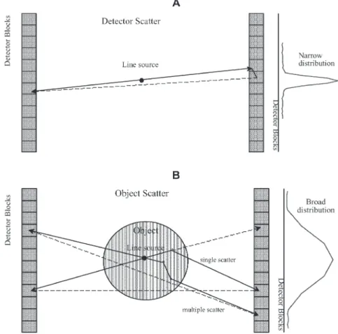
sume that detection can be correctly characterised, and we will not discuss steps in that process. That is, we are declining to distinguish between detection by photoelec-tric absorption and that based upon at least one Compton scatter. Some authors have gone into that process while covering scatter and its correction [2, 3, 4, 5], but we take the point of view that discussing it here would only confuse matters. We feel this point of view is supported by the fact that scatter correction usually does not involve correcting for scatter in the detector crystal. Figure 1 illustrates the difference in terms of origin and shape between object and detector scatter components.
In Compton scattering, the scattered photon emerges from the interaction point with less energy than it had originally, and with a change of direction. The usual physics textbook algebraic equation for the final energy as a function of the initial energy and of the angular change of direction assumes that the interaction was with a free electron at rest [6]. There are corrections to that equation which take into account the fact that the electron actually is moving and is bound to an atom. The result is that the photons that have scattered through a given angle actually have a distribution of energies sharply peaked about the value calculated by the simple formula [7]. Although this effect, which is called Doppler broadening, has some importance for Compton scatter cameras [8], we will not need to discuss it further here
because the energy distribution is so sharply peaked. There are two things about Compton scattering that are important to note for our purposes. One is that the loss of energy can lead to the elimination of a Compton-scat-tered photon by the lower energy window looking at the detected signal. When this happens, the event is no lon-ger of importance for scatter correction. The other is that the change of direction is the basic cause of the problem that calls for correction. Because of the direction change, the detected scattered photon is tracked back incorrectly during reconstruction, if it is assumed to be from an emission site. There will be more discussion of these matters further into this review.
The formula which gives the probability of a Compton scatter from a free electron through a given angle is the Klein-Nishina formula. This formula can also be found in physics textbooks, in an upcoming book that gives a comprehensive view of quantitative nuclear imaging [9] and in many other places.
We have two final introductory points:
1. A Compton-scattered photon can have Compton scat-tered multiple times in either the patient or the colli-mator of the detection system, or a certain number of times (one or more) in the patient, and then a certain number of times (one or more) in the collimator of the detection system.
Fig. 1. A Schematic diagram of the origin and shape of detector scatter component for a cylindrical multi-ring PET scanner geometry estimated from a measurement in air us-ing a line source. B Schematic diagram of the origin and shape of object scatter component estimated from measurements in a cylindrical phantom using a centred line source. Both single and multiple scatter are illustrated
2. The emission site of the original photon may be out-side of the field of view of the scanner.
Sometimes, both of these possibilities are neglected in formulating the correction. In those cases, they can be investigated as additional effects which led to bias in the corrected estimate. Here bias is a statistical term that is defined as a displacement, either up or down, in the strength of a voxel in the resulting image compared with the true (or ideal) value.
Magnitude of scatter
A general idea of the magnitude of collimator scatter and penetration for the range of radionuclides employed in SPECT is given in Table 1. Patient scatter is not involved for 99mTc [10], 67Ga [11] or 131I [12], because
the source was simulated in air. The values for 111In [13]
are appropriate for inclusion in the table, because in that case the definition of a scatter count excluded object scatter (de Vries, personal communication). It can be seen that collimator scatter increases as the energy of the photopeak of interest increases from a low of 1.9% for
99mTc (141 keV) to a high of 29.4% for 131I (364 keV)
with the usual high-energy collimator. The penetration percentage also increases with energy. These same ten-dencies were previously observed in a single study using four different energy emissions from 67Ga [11].
There-fore, correction for photons that penetrate through, or scatter in, collimator septa is hardly important at all for
99mTc, but is potentially important for radionuclides with
higher-energy emissions. Note that an ultra-high-energy collimator with twice the septal thickness can decrease both the collimator scatter and the penetration, as shown by the values for 131I in Table 1. Unfortunately, a similar
table is available neither for a point source in a scattering medium nor for an object containing a distribution of activity. It is, therefore, possible that the dependence on energy could be different in these cases.
A general idea of the magnitude of scatter in myocar-dial imaging is an estimate that the ratio of scattered to unscattered (primary) counts, SP, is approximately 0.34 for 99mTc and 0.95 for 201Tl [14]. The magnitude of
dif-ferent types of events for a 131I source surrounded by a
scattering medium is given in Table 2 (Dewaraja, per-sonal communication). With the standard high-energy collimator, 43% of all detected counts are scattered in either the object or the collimator or both. Also, 27% of all detected counts solely penetrate one or more collima-tor septa. It has been shown for the region of interest and phantom of Table 2 that the spectrum from such pene-trating 364-keV photons is the same as that from the photons that pass along a collimator channel [12] and so one cannot discriminate between the two. One can con-jecture that multi-window scatter correction methods cannot distinguish between the two in general. There-fore, scatter correction for 131I generally does not include
correction for penetration of 364-keV gammas. For the case above, then, 57% of counts (30% passing along a collimator channel plus 27% penetrating one or more septa) are considered “good” counts. That still leaves a Table 1. Magnitude of collimator scatter and penetration for the range of radionuclides employed in SPETa
Source geometry Radionuclide Collimator type Photon’s method of reaching detector (window)
Passed along Penetrated Scattered at collimator one or more least once in channel collimator collimator
septa septa
Small source in air 67Gab(93-keV peak) ME 91.1% 3.4% 2.6%
Point source in air 99mTcc(141 keV) LE 94.5% 3.6% 1.9%
Point source in cold cylinder 111Ind(172-keV peak) Optimal (lead content =14 g/cm2) 89.3% 7.3% 3.4%
111Ind(247-keV peak) 49.9% 34.6% 15.5%
Small source in air 67Ga (300-keV peak) ME 45.6% 32.3% 22.1%
Point source in air 131I (360 keV peak) HE 27.3% 43.3% 29.4%
UHE 72.3% 17.3% 10.3%
LE, Low energy; ME, medium energy; HE, high energy; UHE, ul-tra high energy
aFor all detected photons with an energy signal within the
photo-peak window indicated, the percentage associated with a given path from source to detector is indicated. Counts over the entire projection image were included
bValues do not add up to 100% because for this window there was
a 2.9% contribution to all counts specifically from Pb X-rays pro-duced in the collimator
cThe window was actually set for the 159-keV emission of 123I [10].
Thus it is offset high for the only emission from 99mTc (141 keV) dIn this case, by definition scatter events only included scatter in
the collimator, which could be Rayleigh or Compton scattering (the value is thus lower than it otherwise would be). Therefore, also, the column for “Passed along collimator channel” includes both the counts implied by the label and the counts from photons that scattered in the cylinder (the value is thus higher than it other-wise would be) [13] (de Vries, personal communication)
sizeable 43% needing correction. Note, however, that with the ultra-high-energy collimator, the problem is re-duced: 74% are “good” counts and 26% need correction.
In positron emission tomography (PET), the magni-tude of the included scatter depends heavily on the ac-quisition mode, the body section being imaged (e.g. brain versus thorax versus abdomen or pelvis), and the placement and width of the energy signal acceptance window. The mode depends on whether the field of view for a given detector is restricted in the axial direction (along the z-axis) by the placement of lead or tungsten septa (2D mode), or left considerably more open (3D mode). For standard acceptance windows, in 2D mode the scatter is “10–20% of the total counts acquired” and in 3D mode “approaches half of all recorded events” [15, 16].
It has been shown [17] that in 3D acquisition mode, the variation of the scatter fraction as a function of the phantom size is not linear, reaching a maximum of 66% for a point source located in the centre of a cylindrical phantom (diameter 50 cm, height 20 cm). It is worth em-phasising that the scatter fraction for the same point source in air is higher in 2D (6%) than in 3D mode (2%) owing to the contribution of scatter in the septa in the former case. Another concern in 3D PET in contrast to 2D PET is the scatter contribution from activity outside the field of view and multiple scatter.
Importance of scatter
In the earliest literature on scatter correction, the main import of scatter was considered to be a loss of contrast in the image. In the simplest of descriptions, this means that a true zero in a reconstructed image occurs as a posi-tive value. This effect was demonstrated by imaging non-radioactive spheres in a radioactivity surround [18]. The corruption was frequently described as a pedestal upon which the true image sat. It was soon realised that for quantitative imaging, Compton scatter causes a more
complicated distortion in at least parts of the image. In cardiology with 99mTc, King et al., using Monte Carlo
simulation of a uniformly perfused left ventricle and em-ploying a bull’s eye polar map of counts, pointed out that after attenuation correction using true linear attenuation coefficients the total change in counts due to scatter was 31.3% and that the shape of the distortion was such that there was a slight increase in apparent activity as one moved from the apex of the heart towards the base [14]. So, to the extent that clinicians want an accurate quanti-tative image, including the best contrast possible, scatter is always a problem. The extent to which it can be shown to have a disabling effect upon the goal for which the image is to be employed is a much more difficult matter to discuss and to document. We will try to point out spe-cific instances in this review.
Relationship of scatter to attenuation
In all nuclear medicine imaging (single-photon planar, SPECT and PET), patient scatter is the companion of pa-tient attenuation. That is, a large fraction of the photons that are attenuated instantly fall into the category of a potential scatter-corrupting photon. A photoelectric ab-sorption contributes only to attenuation, but a Compton scatter interaction increases attenuation and also sets up a potential scatter corruption. For the potentiality to be-come a reality, the scattered photon must be detected and also must fall within the energy-signal acceptance win-dow. The sole purpose of that window is to work against the acceptance of scattered photons. An important differ-ence between Compton scatter in SPECT and PET is that in the former, scatter events carry information that can be useful for determination of the body outline or of the non-uniform attenuation map. For example, Pan et al. estimated the regions of the lungs and non-pulmonary tissues of the chest by segmenting the photopeak and Compton scatter window images to estimate patient-spe-cific attenuation maps [19]. Such an approach is ob-Table 2. Magnitude of different types of events for a 131I source surrounded by a scattering mediuma
Collimator type Photon’s method of reaching detector
Passed along collimator Penetrated one or more Scattered at least once in object
channel collimator septa or in collimator septa
HE 30% 27% 43%
UHE 61% 13% 26%
HE, High energy; UHE, ultra high energy
aFor all detected photons with an energy signal within the 20%
photopeak window of the main 364-keV emission of 131I, the
per-centage of the total associated with a given path from source to detector is indicated. The source was a 7.4-cm diameter hot sphere centrally located in a warm cylinder with a diameter of 22 cm and a height of 21 cm. Only counts detected in a circle in the
projec-tion image that corresponded to the sphere were included. N.B. Photons which scattered at least once in the object and also pene-trated collimator septa were included in the scattered percentage. Also, photons which had an emission energy higher than 364 keV and backscattered from material behind the scintillation crystal were included in the scattered percentage, but their numbers were small
viously not possible for PET, where scattered lines of response are sometimes formed outside the body and/or outside the imaging field of view.
For activity quantification, attenuation and scatter have inverse effects on the activity estimate. That is, un-corrected attenuation will allow too few photons to be detected and, therefore, the activity estimate will be too low. Uncorrected scatter corruption will allow too many photons to be detected and, therefore, the activity esti-mate will be too high. The tendency in nuclear medicine has been to separately compensate (or correct) for atten-uation and for scatter. This tendency can be considered a desirable separation of the compensation problem into two simpler parts. It is analogous to plane-by-plane re-construction versus 3D rere-construction. However, with the ability to handle bigger computational loads, it has arguably become advantageous to undertake 3D recon-struction in both SPECT and PET. In SPECT, an exam-ple is the use of 3D collimator-detector response infor-mation during reconstruction. In PET, the advantage of the 3D over the 2D acquisition mode is an increase in the coincidence efficiency by about a factor of 5 even if this is generally accomplished at the expense of increasing the system sensitivity to random and scattered coinci-dences and the complexity and computational burden of the 3D reconstruction algorithm. So, it can arguably be said that the newer methods of handling scatter and attenuation at the same time have potential advantages over the older separate corrections. The most ambitious of these combined corrections, originally called inverse Monte Carlo [20], attempts to reconstruct scattered pho-tons into their voxel of origin. It will be discussed in slightly more detail below. The approach is considered still to be too ambitious to be practical [21]. More practi-cal approaches simply take into account scatter, as well as attenuation, when the forward projection step of an iterative reconstruction iteration is carried out, but “put back” only unscattered photons.
Modelling the scatter component in uniform and non-uniform media
We will define modelling the scatter response as creat-ing a representation of the scatter counts in a projection or sinogram that corresponds to a particular activity dis-tribution in the object as well as to a particular distribu-tion of the linear attenuadistribu-tion coefficients or mass densi-ty in the object. The current practice of developing theo-retical scatter models involves four different stages: characterisation, development, validation and evaluation [22].
1. Characterisation. The scatter response function (srf) is defined as the result of modelling the scatter com-ponent for a simple source distribution, such as a point or line. The srf is studied using a variety
of phantom geometries, source locations, scattering medium shapes, sizes and compositions, as well as imaging system-related parameters (an example of the last-mentioned is the detector energy resolution [23]). The goal is to fully understand and characterise the parameters influencing its behaviour.
2. Development. From knowledge and insight gained during the characterisation step, an appropriate scatter model can be developed, often by using the same tools. This model can be a simple one limited to homogeneous attenuating media, or an elaborate one taking into account more complex inhomogeneous media.
3. Validation. The validation step is the crucial part and involves comparisons between either experimental measurements or Monte Carlo simulation studies and predictions of the theoretical model that has been de-veloped. Monte Carlo simulation is generally prefer-able for practical reasons such as the ease of mod-elling and because it can separate scattered counts from unscattered counts. Again, this validation can be performed using simple phantom geometries (point and line sources in a uniform elliptical cylinder) or more complicated anthropomorphic phantoms that mimic clinical situations.
4. Evaluation. Obviously, evaluation of the theoretical scatter model with respect to its intended use, i.e. scatter correction, constitutes the last step of the whole process. Assessment of the intrinsic perfor-mance of the scatter compensation algorithm that is based on the developed model, as well as its effec-tiveness in comparison to existing methods, is recom-mended.
Accurate simulation of scatter in SPECT/PET projection data is computationally extremely demanding for activity distributions in non-uniform dense media. Such simula-tion requires informasimula-tion about the attenuasimula-tion map of the patient. A complicating factor is that the scatter re-sponse is different for every point in the object to be imaged. Many investigators have used Monte Carlo techniques to study the scatter component or srf [17, 24, 25, 26, 27, 28]. However, even with the use of variance reduction techniques, these simulations require large amounts of computer time. Moreover, the simulation of the srf for each patient is impractical.
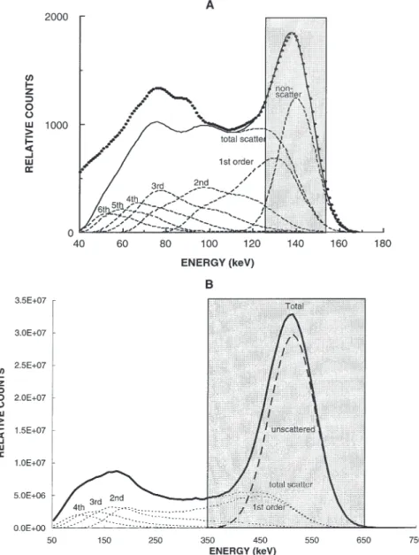
Figure 2 shows the energy pulse-height distribution obtained by simulation of a gamma-emitting 99mTc line
source in the centre of a water-filled cylindrical phan-tom and a uniform positron-emitting 18F cylindrical
source. The scattered events in the energy pulse-height distribution have been separated according to the order of scattering. It is clear from viewing Fig. 2 that events from some scattered photons will not be rejected by the usual [126–154 keV] and [350–650 keV] energy discrimination, in SPECT and PET, respectively, due to the limited energy resolution. Scattered photons which
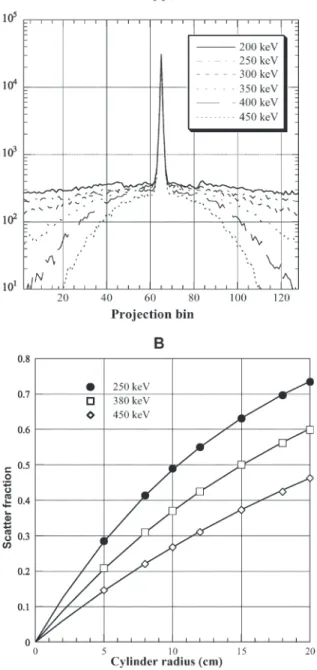
fall within the photopeak window consist mainly of photons which have only scattered once (first order). The lower level threshold (LLT) can be easily changed and its effect on the scatter component studied in an effective way. Figure 3 shows transaxial profiles in the projection space for PET simulations of a line source in a 20-cm-diameter water-filled cylinder as a function of the LLT. In each case, the centre of the cylinder is located at the origin of the graph. It is clear that the boundary (at −10 cm, +10 cm) of the object has no in-fluence on the profile. However, the value chosen for the LLT greatly influences the amount of scatter in the projection data.
Scatter is often measured by imaging a line source placed at the centre of a water-filled cylinder. Line spread srfs (LSFs) are generated and the scatter fraction (SF) determined by fitting the scatter tails of the LSFs to a mono-exponential function. The scatter fraction is de-fined as scatter divided by total counts recorded, where
total and scatter are calculated as the integral of the LSF and the fit to the tails, respectively. The variation of the scatter fraction was investigated for a line source located at the centre of a uniform cylindrical phantom as a func-tion of its size and for three lower energy thresholds (250, 380 and 450 keV). The second part of Fig. 3 shows the scatter fraction estimated directly from the results of the Monte Carlo simulation [29] where the simulated PET scanner operating in 3D mode has an axial field of view of 16.2 cm and an energy resolution of 23% for 511-keV photons.
Adam et al. used Monte Carlo simulations to study scatter contribution from outside the field of view and the spatial characteristics of scatter for various phantoms [17]. It was concluded that the spatial distribution of multiple scatter is quite different from the simple scatter component and that this fact precludes the rescaling of the latter to take into account the effect of the former for scatter correction purposes.
Fig. 2. A An energy spectrum for a gamma-emitting 99mTc
line source on the axis of a water-filled cylinder simulated using the Monte Carlo method. The spectrum due to primary and scattered photons (solid line) is separated into different contributions (total scattering or different orders of photon scattering). The distributions of the various orders of scattered and unscattered photons are shown by broken lines. The experimentally measured spec-trum is also shown (dots). B Illustration of the energy distribution due to unscattered and scattered photons resulting from the simulation of a 20-cm-diameter cylinder filled with a uniform positron-emit-ting 18F source separated into
different contributions (total scattering or different orders of photon scattering). Typical energy acquisition windows for both cases are also shown. (Adapted from [23] and [72])
Analytical scatter models, based on integration of the Klein-Nishina (K-N) equation [30, 31, 32], have practi-cal disadvantages, which are similar to those of Monte Carlo-based methods [33, 34, 35].
One class of methods, which estimates anatomy-de-pendent scatter, first calculates and stores in tables the
scatter responses of point sources behind slabs for a range of thicknesses, and then tunes these responses to various object shapes with uniform density [36]. This method is referred to as slab-derived scatter estimation (SDSE). A table occupying only a few Mbytes of memory is sufficient to represent this scatter model for fully 3D SPECT reconstruction [37]. A fully 3D reconstruction of a 99mTc cardiac study based on SDSE can be performed
in only a few minutes on a state-of-the-art single-proces-sor workstation. A disadvantage of SDSE compared with matrices generated by Monte Carlo simulation or Klein-Nishina integration is that it cannot accurately include the effects of the non-uniform attenuation map of the emitting object density.
A few rough adaptations have been proposed to im-prove the accuracy and computational speed of this method [38, 39, 40] or other similar approaches [41] in non-uniform objects. SDSE has also been modified to be applicable to 201Tl and to non-uniform attenuators such
as found in the chest by its authors. The new approach [42] is called effective source scatter estimation (ESSE). It can perhaps be best described briefly by quoting from the authors’ abstract: “The method requires 3 image space convolutions and an attenuated projection for each viewing angle. Implementation in a projector–backpro-jector pair for use with an iterative reconstruction algo-rithm would require 2 image space Fourier transforms and 6 image space inverse Fourier transforms per itera-tion.”
For implementation, after the effective source of the method’s name is generated: “An attenuated projector that models the distance-dependent collimator-detector response blurring was then applied to this effective source to give the scatter estimate.” The authors further say: “We observed good agreement between scatter re-sponse functions and projection data estimated using this new model compared to those obtained using Monte Carlo simulations.”
Beekman et al. [43] reported an accurate method for transforming the response of a distribution in a uniform object into the response of the same distribution in a non-uniform object. However, the time needed to calcu-late correction maps for transforming a response from uniform to non-uniform objects may be too long for rou-tine clinical implementation in iterative reconstruction-based scatter correction, especially when the correction maps are calculated for all projection angles and each iteration anew. The use of only one order of scatter was sufficient for an accurate calculation of the correction factors needed to transform the scatter response. Since the computation time typically increases linearly with the number of scatter orders, this transformation method yields much shorter computation times than those with straightforward Monte Carlo simulation. The method was also extended to simulate downscatter through non-uniform media in dual-isotope 201Tl/99mTc SPECT
imag-ing [44]. Fig. 3. A Sum of one-dimensional transaxial projections resulting
from the simulation of a line source placed in a 20-cm-diameter cylinder filled with water as a function of the lower energy dis-crimination threshold. This illustrates the compromise that should be attained between increasing the lower level threshold to reduce scattered events and the variance in the reconstructed images re-sulting from limited statistics. B Monte Carlo calculations of the variation of the scatter fraction as a function of the radius R of the cylindrical phantom for a central line source using three different LLT settings. The fitted curves are also shown
Scatter correction techniques in SPECT
The older SPECT scatter correction techniques have been reviewed frequently [3, 45, 46] and many of the newer ones have been included in the newer reviews [9, 47]. Therefore, rather than giving each correction method the same amount of space, we are going to neglect some older methods covered in the reviews cited and will present long descriptions only for the newer methods and/or for those not extensively covered in the reviews cited. In addition to describing correction methods, we will discuss comparisons of one method to another, and review studies that present evidence of the clinical impact of scatter correction.
Implicit methods
Scattered photons degrade the point-spread function (PSF) of the SPECT camera; the long tails of the PSF are mainly due to scatter. Thus, deconvolution methods, which correct the images for the PSF, will also implicitly correct for scatter. In general, the PSF will act as a low-pass filter. Deconvolution will restore the high-frequency contents. However, not only the high frequencies in the signal are restored, but also the high-frequency noise is amplified, which in turn can degrade the image. There-fore, the restoration filter is often combined with a low-pass filter that balances that image improvement by de-convolution and its degradation due to amplification of noise. Well-known examples of these filters are the Wiener and Metz filters. Several investigators have anal-ysed these filters in nuclear imaging and compared their performance relative to each other and relative to other filters and scatter correction approaches [48, 49].
Methods requiring a transmission measurement
The transmission-dependent convolution subtraction (TDCS) method was introduced in 1994 [50]. It was de-veloped for 99mTc [51] and 201Tl [52]. As described in an
earlier review [9], “It draws upon earlier approaches, and is basically an iterative procedure although sometimes only one iteration is used. It also takes the geometric mean of conjugate views, relies on a convolution, uses a ratio of scattered events divided by total events, SF(x,y), and employs a depth-dependent build-up factor, B(d). The SF(x,y) and the B(d) are both variable across the two-dimensional projection image”. The basic equation is:
(1) Here, is the scatter corrected emission projection data after the nthiteration, is the observed
photo-peak projection data without scatter correction,
is the scatter corrected projection data after the (n–1)th
iteration and x is a transverse coordinate while y is an axial one. The two-dimensional convolution operation is performed in projection space after taking the geometric mean and the srf(x,y) is radially symmetrical and was originally assumed to be an exponential [50]. The SF(x,y) is defined in terms of B(d), which is itself ex-pressed in terms of measured parameters, A, α and β, and the narrow-beam transmission function,T(x,y):
(2) Narita et al. used ten iterations whereas only one was originally employed [51]. They also made several small changes by using a scatter function that was the sum of an exponential plus a Gaussian, and by averaging the dependence of SF on the transmission factor from two empirical cases. Kim et al. also modified the original method when they wanted to use it for 123I brain imaging
[53]. In their study, the original equation for SF as a function of transmission was modified to include a con-stant additive term. This term was needed to account for septal penetration of a small percentage of photons from
123I that have energies greater than 500 keV [53]. They
carried out studies of a phantom and of six patients. The need for more than one iteration in the TDCS method comes about because originally an image recon-structed from the observed projections is used to gener-ate the scatter correction image whereas the true scatter-free image theoretically would give the correct answer [9]. Moreover, in a recent note it has been argued that in addition to using multiple iterations, a matrix of SP val-ues should replace the matrix of SF valval-ues as the image approaches the scatter-free image [54]. The authors of the note carried out a test of their suggestion by simulat-ing a 99mTc point source centrally positioned in a
rectan-gular water phantom of dimensions 20×20×20 cm3. They
used an exponential shape for the scatter kernel. They found a better result by using the SF value only for the first iteration and then the SP value for the succeeding nine iterations, compared with using the SF value for either only one iteration or for all ten iterations.
Multiple-energy window (spectral-analytic) approaches The multi-energy window approaches include the dual-energy window (DEW) method, the split-photopeak win-dow method, the triple-energy winwin-dow (TEW) approach, the spectral fitting method, a multi-window method with weights optimised for a specific task and the neural-network methods. The first involves a window usually of equal width to the photopeak window, placed at a lower energy immediately abutting the photopeak [18]. The second involves splitting the photopeak into two equal halves and using information from the relative number of counts in each half [55]. The TEW method [56] uses the photopeak window and two narrower windows, one
higher and one lower in energy. The spectral fitting method [57] involves establishing the shape of the energy spectrum for unscattered counts (the scatter-free spectrum). The full energy spectrum, which must be measured over some energy range for each pixel (or “superpixel”), usually by list-mode acquisition, is then assumed to be a value times that scatter-free spectrum plus a spectrum for the scattered photons. For each pixel, the multiplicative value and the spectrum for the scat-tered photons are obtained by finding the least squares fit between the measured composite spectrum and the as-sumed components. Variations on the basic approach exist [58].
In the task-specific multiple-window method, weights for each energy window are determined using an optimi-sation procedure [1, 59]. In the case of brain imaging with 99mTc, the chosen task was both accurate lesion and
non-lesion activity concentration. The resultant weights had both positive and negative values. In operation, they are combined with the measured spectrum to produce the estimate of total primary counts [1].
A multi-window approach that employs training is scatter estimation using artificial neural networks. These were introduced for scatter correction in 1993 [60]. The reader is referred to that study, to newer studies [61, 62] and to a review [9] for details because the approach can-not be described in a few words.
Approaches requiring iterative reconstruction
In emission tomography, the scatter estimate can be either precomputed and simply used during iterative reconstruction or generated as well as used during itera-tive reconstruction [63]. By the former we refer to not explicitly subtracting the scatter estimate from the ob-served projection data, but simply including it in the sta-tistical model [64]. That is, the goal of a given iteration becomes finding the object that, when it is forward pro-jected and the scatter estimate is added, best fits the mea-sured projection data, with “fit” quantified by the log-likelihood of the Poisson statistical model. In that model, the variance equals the mean, and the mean includes both the unscattered and the scattered contributions.
One class of correction methods uses Monte Carlo simulations [20, 21] to compute the complete transition matrix (aij), including scatter events. This matrix repre-sents the mapping from the activity distribution onto the projections. Since the first guess of the activity distribu-tion is unlikely to be right, no matter how it is derived, the approach is iterative. Monte Carlo simulation can readily handle complex activity distributions and non-uniform media. Unfortunately, a large amount of memo-ry is required to store the complete non-sparse transition matrix when the fully 3D Monte Carlo matrix approach is used, and without approximations it can take several weeks to generate the full matrix on a state-of-the-art
workstation. In addition, the procedure has to be repeat-ed for each patient.
Another class of methods improves the efficiency by utilising a dual matrix approach in which scatter is incor-porated in the forward projection step only of an iterative reconstruction algorithm such as the maximum-likeli-hood expectation-maximisation (ML-EM) or its acceler-ated version, the ordered-subsets expectation-maximisa-tion (OS-EM) [65].
One of the requirements of this method is the compu-tation of the srf at each point in the attenuator for all pro-jection views and for each iteration. To avoid slow com-putation, the correction factors could be calculated only once or alternatively a few times only, given that the cal-culated scatter component does not change much after the first few iterations of accelerated OS-EM statistical reconstruction have been carried out [43]. Thus, the scat-ter estimate can be kept as a constant scat-term in either all or only later iterations instead of modifying the scatter esti-mate in each iteration [40, 64]. In this way, a constant pre-calculated scatter component (using one of the meth-ods described above) can be introduced in the denomina-tor, i.e. the forward projection step of the ML-EM equa-tion:
(3) where piand fjare the discrete set of projection pixel val-ues and counts originating from the object voxel activity concentration, respectively, and is the scatter estimat-ed on all projections.
Interest in this type of approach has been revived with the development of a computationally efficient approach to preserve the main advantages of iterative reconstruc-tion while achieving a high accuracy through modelling the scatter component in the projector using Monte Carlo-based calculation of low-noise scatter projections of ex-tended distributions, thus completely avoiding the need for massive transition matrix storage [35].
Impact of scatter correction on clinical SPECT imaging
At the time of the review by Buvat et al. in 1994, their opinion was that the most clinically used scatter correc-tion method in SPECT was employment of a decreased attenuation coefficient; that is, to not increase recon-structed strength sufficiently during attenuation correc-tion, so as to compensate for not carrying out a reduction in strength to compensate for inclusion of scattered counts. One of the reasons they gave for use of this infe-rior approach was as follows: “Although most methods have been assessed using simulated and physical data, none has yet faced an extensive procedure of clinical as-sessment” [3]. However, from the studies cited below in
this section, it arguably appears that at least a start on the extensive procedure of clinical assessment has recently been made.
Since the comment by Buvat et al. in 1994, other methods, but still straightforward ones, particularly the DEW method and the TEW method, have become the ones most used in SPECT imaging of patients. For ex-ample, Narayanan et al. [66] say the TEW method is their “current clinical standard,” and Koral et al. use TEW correction in their clinical SPECT assessment of tumour activity [67]. However, the DEW method is known to be wrong when it uses a spatially invariant value for the ratio of the corrupting scatter counts in the photopeak window to the total counts in the lower-ener-gy monitor window, the k factor [47]. In addition, the narrow monitoring windows in the TEW approach are suspected of generating noisy estimates of the scatter correction image. So, the question is: Can any method prove itself so much better as to displace these, older, simpler methods, or will they continue to be used despite their known or possible shortcomings? Probably the answer will lie in how much effort is devoted to estab-lishing a newer and/or more complicated method in the future.
To date, the TDCS method has been tested for brain and heart imaging [51, 52]. In 123I brain imaging, Kim et
al. [53] found that their version of the TDCS provided “an acceptable accuracy” in the estimation of the activity of the striatum and of the occipital lobe background. Moreover, parameter values averaged over six collima-tors from three different SPECT cameras yielded “mini-mal differences” among the collimators, so new users might not have to calibrate their collimator–camera system.
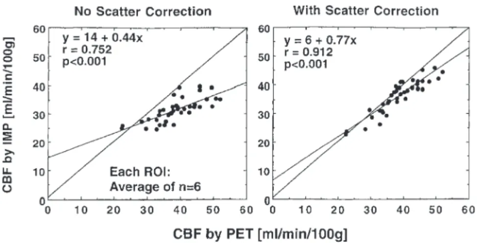
In a study by Iida et al., it was conclusively found that the regional cerebral blood flow (rCBF) from 123
I-iodoamphetamine (IMP) SPECT imaging correlated bet-ter with the values from 15O-water PET imaging when
TDCS scatter correction was employed than when no scatter correction was performed [68]. This fact is shown in Fig. 4 reproduced from the study. The correlation
co-efficient is 0.912 with correction but only 0.752 without. Also, the slope of the best-fit line is 0.77 with correction but only 0.44 without.
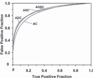
In SPECT cardiology, Narayanan et al. carried out a human observer study using clinical data from 100 pa-tients undergoing 99mTc-sestamibi perfusion studies
[66]. Three cardiology fellows were trained and provid-ed the raw data for the receiver-operating-characteristics (ROC) study. Two methods of scatter correction were separately tested in combination with attenuation cor-rection and detector–collimator response compensation. They were compared with filtered backprojection. Five iterations of OS-EM using 15 subsets were employed for reconstructions with scatter correction, and the scatter estimate was used during the reconstruction rather than subtracted from the projection data (see the section on “Approaches requiring iterative reconstruc-tion” for further explanation of this type of procedure). There are more comments on the two methods in the section on comparison of corrections below. Both meth-ods provided statistically significant improvement for the overall detection of coronary artery disease com-pared with filtered backprojection. Both also provided larger areas under the ROC curve for localisation of a perfusion defect to the left anterior descending (LAD) territory, to the left circumflex territory (LCx) and to the right coronary artery (RCA) territory. The improvement was statistically significant for the LAD and LCx terri-tories. Significance was computed using the “two-way ANOVA test for statistical significance, followed by Scheffe’s multiple comparisons test” using the usual limit of 5%. This study is impressive to the authors of this review. The only qualification that perhaps needs to be made is that only 55 of the 100 patients had cardiac catheterisation. The remaining 45 subjects were deemed to have a ≤5% likelihood for CAD. Not being experts in the cardiac area, we do not know how reasonable this 5% likelihood is. Also, we did not see a justification for it in the article, although it probably rests on the clinical assessment that resulted in the patients not being sent for cardiac catheterisation.
Fig. 4. Plot of rCBF assessed by 123I-IMP SPECT versus that
measured by the gold-standard,
15O-water PET imaging. On the
left, the SPECT values are without scatter correction. On the right, the SPECT values are with TDCS scatter correction. Each value corresponds to the average over six patients for a particular region of interest in the brain. (Reprinted with permission from [68])
Scatter correction techniques in PET
Unlike the scatter correction strategies employed in SPECT, those used in PET have been discussed only briefly [15, 69, 70] with the exception of the extensive reviews provided in book chapters [9, 71, 72]. Over the past two decades, many methods have been developed for the purpose of reducing the degradation of image contrast and loss of quantitative accuracy in PET due to scattered events. The main difference among the correc-tion methods is the way in which the scatter component in the selected energy window is estimated. The most re-liable method to determine the actual amount of scatter in the image is accurate modelling of the scatter process to resolve the observed energy spectrum into its unscat-tered and scatunscat-tered components. By observing how accu-rately a scatter correction algorithm estimates the amount and distribution of scatter under conditions where it can be accurately measured or otherwise inde-pendently determined, it is possible to optimise scatter correction techniques. A number of scatter correction al-gorithms for PET have been proposed in the literature. They fall into four broad categories [15, 71]:
– Multiple-energy window (spectral-analytic) approaches – Convolution/deconvolution-based approaches
– Approaches based on direct estimation of scatter dis-tribution
– Statistical reconstruction-based scatter compensation approaches
Different versions of the above methods have been suc-cessfully implemented for 3D PET and are briefly dis-cussed below.
Multiple-energy window (spectral-analytic) approaches The development of 3D acquisition mode and improve-ments in the detector energy resolution in PET have al-lowed the implementation of scatter correction based on the analysis of energy spectra. Several groups investigat-ed the potential of acquiring data in two [73, 74], three [75] and multiple [4] energy windows to develop correc-tions for scattering in 3D PET. Two variants of the SPECT DEW technique have been proposed for PET: methods estimating the scatter component in the photo-peak window from the events recorded in a lower energy window placed just below the photopeak (true DEW) and methods estimating the unscattered component in the photopeak window from the unscattered counts recorded in a high-energy window in the upper portion of the photopeak. The DEW technique of Grootoonk et al. [73] belongs to the former while the estimation of trues method (ETM) [74] belongs to the latter.
The DEW method implemented on the ECAT 953B scanner (CTI/Siemens) assigns detected coincidence
events to the upper energy window when both photons deposit energy between 380 keV and 850 keV, or to the lower energy window when one or both photons deposit energy between 200 keV and 380 keV [73]. Both energy windows are assumed to contain object scattered and un-scattered events. Based on data collected in the two ener-gy windows and scaling parameters derived from mea-surements of the ratios of counts from line sources due to unscattered (measurements in air) and scattered events (measurements in a head-sized phantom), two equations containing four unknown parameters are solved to esti-mate the unscattered component in the acquisition energy window.
The ETM method [74] consists in acquiring data si-multaneously in two energy windows: a high window with a lower energy threshold higher than 511 keV and a regular acquisition window including the higher window. Therefore, both windows have the same upper level threshold (ULT) value. In the window choice, the method is like the SPECT dual-photopeak window method. The hypothesis of the ETM method is that the number of un-scattered coincidences recorded in a given energy range depends on the energy settings of the window and the angle of incidence of the annihilation photons on the de-tector face. Hence, the unscattered component in the high-energy window can be related to the unscattered co-incidences in the standard wider window through a func-tion of the energy settings, the radial posifunc-tion in the sino-gram for a given line of response and the axial opening for a given radial position. This calibrating function is assumed to be independent of the source distribution. The unscattered component in the wide energy window can thus be calculated and subsequently subtracted from the data recorded in the regular window to produce a scattered sinogram. The unscattered component in the regular window is then obtained by smoothing that sino-gram and subtracting it from the data recorded in the standard window.
The TEW method [75] was suggested as an extension of the DEW technique. Coincidence events are recorded in three windows: two overlapping windows having the same ULT settings (450 keV) and located below the pho-topeak window and a regular window centred on the photopeak and adjacent to the low windows. A calibrat-ing function that accounts for the distribution of scat-tered coincidences at low energies is obtained by calcu-lating the ratio of the coincidence events recorded in both low-energy windows for the scanned object and for a homogeneous uniform cylinder. The scatter component in the standard acquisition window is then estimated from the calibrating function and the narrower low-energy window.
The multispectral method is based on the acquisition of data in a very large number (typically 256) of win-dows of the same energy width (16×16 energy values for the two coincident photons). The spatial distribution of scattered and unscattered components in each window
can be well fit using simple mono-exponential functions [4]. It has been shown that “while subtraction of object scatter is necessary for contrast enhancement and quanti-tation accuracy, restoration of detector scatter preserves sensitivity and improves quantitation accuracy by reduc-ing spillover effects in high-resolution PET” [76]. The statistical noise in each window is a potential problem. The hardware and software for multiple-window acquisi-tion remain the major obstacles to implementaacquisi-tion of the method on commercial PET scanners.
Convolution–deconvolution based approaches
Techniques based on convolution or deconvolution esti-mate the distribution of scatter from the standard photo-peak data. The SF, which gives an indication of the ex-pected amount of scatter, and the srf, which defines the spatial distribution of scatter, are usually the two param-eters that need to be determined a priori. A pure additive model of the imaging system in which the recorded data (po) are composed of an unscattered (pu) and a scattered (ps) component plus a noise term due to statistical fluctu-ations is generally assumed. The problem to be ad-dressed consists in estimating pufrom pothat is contami-nated by scatter, or alternatively estimating ps and then calculating pu. The proposed methods differ in the way the srf is defined.
The convolution-subtraction (CVS) technique devel-oped for 3D PET [77] operates directly on projection data (pre-reconstruction correction). The method is generally based on convolving the source distribution with the srf to obtain an estimate of the scatter component. One makes one of two assumptions: the stationary or the non-stationary assumption. With the non-stationary assumption, the srf is assumed to be analytically defined and not de-pendent on the object, activity distribution, etc. Because this assumption is only approximately correct, an iterative procedure is generally used. The rationale is that with each iteration, the input to the scatter estimation step more closely approximates pu. Using a damping factor to prevent oscillations in the result has also been suggested [77]. With the non-stationary assumption, one improves on the previous approximation by taking into considera-tion the dependence of the srf upon source locaconsidera-tions, ob-ject size, detector angle, etc. There is a continuing interest in developing the non-stationary CVS scatter correction techniques. Different methods have been proposed in the literature for SPECT [25] and 2D PET imaging [5]; the extension of such models for 3D PET should in principle be straightforward. The CVS approach can also be ap-plied to the reconstructed images (post-reconstruction correction). In this case, the scatter estimates are recon-structed and then subtracted from the non-corrected re-constructed images of the acquired data [78].
The curve-fitting approach is based on the hypothesis that detected events assigned to lines of response outside
of the source object must have scattered and that the scatter distribution corresponds to a low-frequency com-ponent that is relatively insensitive to the source distri-bution. Estimation of the unscattered component can thus be performed in three successive steps: (a) fitting the activity outside the source object with an analytical function (e.g. Gaussian), (b) interpolating the fit inside the object and (c) subtracting the scatter component from the observed data [79]. The accuracy of this class of scatter correction methods depends on how accurately the scatter component can be estimated. The appropriate choice of a set of fitting parameters, which should be op-timised for each PET scanner and for different distribu-tions of radioactivity and attenuation coefficients, is the dominant factor.
Links et al. [80] studied the use of two-dimensional Fourier filtering to simultaneously increase quantitative recovery and reduce noise. The filter is based on the in-version of the scanner’s measured transfer function, cou-pled with high-frequency roll-off. In phantom studies, they found improvements in both “hot” and “cold” sphere quantification. Fourier-based image restoration filtering is thus capable of improving both accuracy and precision in PET.
Approaches based on direct calculation of scatter distribution
This class of methods assumes that the distribution of scattered events can be estimated accurately from either the information contained in the emission data or that in both the emission data and the transmission data. For the majority of detected scattered events, only one of the two annihilation photons undergoes a single Compton interaction. The rationale for most methods in this class is that the overall scatter distribution can be computed from the single-scatter distribution (~75% of detected scattered events) and that this latter can be scaled to model the distribution of multiple-scattered events [81]. The multiple-scatter distribution is generally modelled as an integral transformation of the single-scatter distribu-tion. Monte Carlo simulation studies of various phantom geometries demonstrated the potential and limitations of this method for fully 3D PET imaging by direct compari-son of analytical calculations with Monte Carlo esti-mates [17, 26].
The model-based scatter correction method developed by Ollinger [81] uses a transmission scan, an emission scan, the physics of Compton scatter and a mathematical model of the scanner for use in a forward calculation of the number of single-scatter events. Parameterisation of a fast implementation of this algorithm has recently been reported [82]. The main algorithm difference from that implemented by Ollinger [81] is that “the scatter correc-tion does not explicitly compute scatter for azimuthal an-gles; rather, it determines 2-D scatter estimates for data
within 2-D ‘super-slices’ using as input data from the 3-D direct-plane (non-oblique) slices”. A single-scatter simulation (SSS) technique for scatter correction where the mean scatter contribution to the net true coincidence data is estimated by simulating radiation transport through the object was also suggested and validated using human and chest phantom studies [32]. The same author reported on a new numerical implementation of this algorithm, which is faster than the previous imple-mentation, currently requiring less than 30 s execution time per bed position for an adult thorax [83]. The nor-malisation problem was solved and multiple scatter par-tially taken into account. However, the above methods do not correct for scatter from outside the field of view.
Contribution of scatter from outside the FOV remains a challenging issue that needs to be addressed carefully in whole-body imaging, especially with large axial FOV 3D PET scanners. Scatter from outside the field of view can be directly taken into account by acquiring short, auxiliary scans adjacent to the axial volume being inves-tigated. This technique implicitly assumes that the distri-bution of scatter from outside the FOV has the same shape as that of scatter from inside the FOV. These extra data are naturally available in whole-body imaging. However, this method is impractical for isotopes with a short half-life or rapid uptake relative to the scanning in-terval. It has also been shown that the attenuation map to be used as input for estimation of the scatter distributions can be derived from magnetic resonance images in brain PET scanning [84]. The contribution of scatter from outside the FOV might be handled effectively using a hybrid approach which combines two scatter correction methods in a complementary way such that one method removes a proportion of scattered events which are not modelled in the second one and vice versa. For example, Ferreira et al. [85] have combined the energy-based ETM algorithm (to remove scatter from outside the FOV) and either CVS or SSS (to remove small-angle scatter) to improve the contrast.
The experimental measurement of the true scatter component is impossible, but it can be accurately esti-mated using rigorous Monte Carlo simulations. Given a known radioactive source distribution and the density of the object, Monte Carlo techniques allow detected events to be classified into unscattered and scattered events and thus the scatter component to be determined. However, the source and scattering geometry is generally not known in clinical studies. In their Monte Carlo-based scatter correction (MCBSC) method, Levin et al. used filtered backprojection reconstructions to estimate the true source distribution [33]. This input image is then treated as a 3D source intensity distribution for a photon-tracking simulation. The number of counts in each pixel of the image is assumed to represent the isotope concen-tration at that location. The image volume planes are then stacked and placed at the desired position in the simulated scanner geometry, assuming a common axis.
The program then follows the history of each photon and its interactions in the scattering medium and traces es-caping photons in the block detectors in a simulated 3D PET acquisition. The distributions of scattered and total events are calculated and sorted into their respective sinograms. The unscattered component is equal to the difference between measured data and the scaled and smoothed scattered component. To reduce the calcula-tion time, coarser sampling of the image volume was adopted, assuming that the Compton scatter distribution varies slowly over the object. For obvious reasons, the implemented method does not correct for scatter from outside the field of view and further refinements of the technique were required to take this effect into account. A modified version of this approach was therefore suggested [86]. The data sets were pre-corrected for scatter and the reconstructed images were then used as input to the Monte Carlo simulator [29]. This approach seems reasonable for a more accurate estimation of the true source distribution. Faster implementations of similar approaches have also been described elsewhere [34].
Iterative reconstruction-based scatter correction approaches
Development of scatter models that can be incorporated into statistical reconstruction such as OS-EM for PET continues to be appealing; however, implementation must be efficient to be clinically applicable. It is worth-while to point out that, with few exceptions [28, 87, 88], most of the research performed in this field is related to SPECT imaging as reported previously. In the study by Werling et al. [88], the preliminary results obtained using a fast implementation of the SSS algorithm [83] were not satisfactory, and thus spurred further research to incorpo-rate a more accuincorpo-rate model that took into account multi-ple scatters. Further development and validation of this class of algorithms in whole-body 3D PET are still needed.
Another technique for scatter correction in 3D PET, called statistical reconstruction-based scatter correction, was also recently proposed [28]. The method is based on two hypotheses: (a) the scatter distribution consists mainly of a low-frequency component in the image, (b) the low-frequency components will converge faster than the high-frequency ones in successive iterations of statistical reconstruction methods. This non-uniform convergence property is further emphasised and demon-strated by Fourier analysis of the ML-EM algorithm [89] and successive iterations of inverse Monte Carlo-based reconstructions [20]. The low-frequency image is esti-mated using one iteration of the OS-EM algorithm. A single iteration of this algorithm resulted in similar or better performance than four iterations of the CVS method [86].
Impact of scatter correction on clinical PET imaging
There is little in the literature reporting systematic stud-ies on the clinical impact of different scatter correction techniques versus no correction in 3D PET. It is well known that subtraction-based scatter correction increases statistical noise. However, in general scatter correction improves the contrast compared with the case where no correction is applied. In particular, the low-count regions and structures are better recovered after scatter
compen-sation. Figure 5 illustrates typical clinical 18F-FDG brain
and thoracic PET scans reconstructed without and with scatter correction, respectively. The data were acquired on the continuously rotating partial-ring ECAT ART to-mograph (CTI/Siemens) and corrected for attenuation using collimated 137Cs point source-based transmission
scanning. Scatter correction improves the contrast be-tween the different brain tissues and removes back-ground counts in the abdomen and lungs. The myocardi-um is also better delineated after scatter compensation. Thus, there is consensus within the nuclear medicine Fig. 5. Examples of clinical
PET images reconstructed without (left) and with (right) scatter correction for typical
18F-FDG brain (A) and
whole-body (transaxial and coronal slices) (B) scanning. Note that scatter correction improves the contrast between the grey matter, the white matter and the ventricles in brain imaging and removes background counts in the abdomen and lungs in myocardial imaging. The myocardium is also better delineated after scatter correc-tion. The brain images were corrected for attenuation and reconstructed using an analyti-cal 3DRP algorithm while the whole-body images were re-constructed using normalised attenuation weighted, OS-EM iterative reconstruction (two iterations, eight subsets) followed by post-processing Gaussian filter
community with respect to the potential usefulness and necessity of scatter correction for either qualitative inter-pretation of patient images or extraction of clinically useful quantitative parameters. The main application which is still the subject of debate is 15O[H
2O] brain
ac-tivation studies characterised by low-count imaging pro-tocols, where scatter subtraction might jeopardise the power of statistical analysis significance. In these cases, PET studies focus on identification of functional differ-ences between subjects scanned under different condi-tions. Whether the scatter component can be considered as constant between the two conditions for inter-subject comparisons still needs to be demonstrated. This con-stancy is required to confirm the hypothesis that the out-come of statistical analysis (reflecting subtle changes in distribution of radiotracer) does not change greatly with and without scatter compensation.
In radiotracer modelling studies, differences of 10–30% in the kinetic parameters derived from patient studies are often found to be significant [79]. The magni-tude of the scatter correction may cause some parameter values to increase several-fold, with an associated in-crease in noise. Application of such a correction, if the increase in noise cannot be prevented, would jeopardise the ability to detect subtle biological effects.
Evaluation of scatter correction approaches Comparison of methods
In either SPECT or PET, it has been difficult to establish the superiority of one method over another. The main difference between the correction methods is the way in which the scatter component in the selected energy win-dow is estimated. A limited number of studies reported the comparative evaluation of different scatter correction methods in both SPECT [37, 90, 91, 92] and PET [86, 93, 94] imaging. There is no single figure of merit that summarises algorithm performance, since performance ultimately depends on the diagnostic task being per-formed. Well-established figures of merit known to have a large influence on many types of task performance are generally used to assess image quality [95]. Many papers dealing with the evaluation of scatter correction tech-niques compare relative concentrations within different compartments of a given phantom with the background compartment serving as a reference. This approach pos-sibly obscures what is actually going on, does not neces-sarily reflect the accuracy of the correction procedure and might bias the evaluation procedure [71]. Therefore attempts should be made to evaluate results in absolute terms.
Ljungberg et al. looked at four methods for scatter cor-rection with 99mTc [90]. They were the DEW method, the
split-photopeak method, a version of the TEW method where only two windows are actually employed and a
method based on scatter line-spread functions. The test-ing involved a brain phantom and employed Monte Carlo simulation. The results indicated “...that the differences in performance between different types of scatter correction technique are minimal for Tc-99m brain perfusion imag-ing.” Thus, in 1994 using filtered backprojection recon-struction with a pre- and post-filter, comparing four par-ticular methods, the conclusion was that there was no dif-ference.
Buvat et al. examined nine spectral or multi-energy window methods, again for 99mTc. They simulated a
single, complex phantom [91]. The authors made a con-siderable number of detailed observations in comparing the nine different scatter compensation methods, some of which were closely related. They also made the impor-tant distinction of judging the methods based on relative quantification and on absolute quantification. Based on relative quantification, the TEW approach, simplified for
99mTc, and two factor analysis methods yielded the best
results. However, the same methods were not the best based on absolute quantification. That is, in a plot where each value pair represented the estimated and true num-ber of scattered counts in a pixel, the DEW correction method yielded the result which most closely followed the line of identity. Buvat et al. commented on other con-siderations, such as a greater need for energy linearity in physical cameras for certain methods. They also came to additional conclusions, not all of which are as transpar-ently justified to the authors of this review as those pre-sented above.
Three studies referred to earlier compared new SPECT scatter correction method with the TEW method. Narita et al. compared results from their version of TDCS with the results from TEW scatter correction and concluded that their method produced a much smoother scatter estimate, and that the resulting signal to noise ratio was better than with TEW correction [51, 52].
Iida et al. [68], in the study referred to earlier, com-pared the TDCS method with the TEW method in the same patients (in both cases, the attenuation correction approach was based on a transmission scan of the pa-tient). The result for rCBF for one particular patient is shown in Fig. 6, reproduced from their study. The authors state: “The increased image noise in the TEW corrected images is clearly apparent.” We basically agree with the authors but would qualify the statement by pointing out that what is most striking to us in the com-parison is how closely the results are the same. Also, in one part of the authors’ work they carried out a detailed comparison between TDCS and TEW while holding the method of attenuation correction constant. Table 2 of the publication presents the rCBF in ml/min/100 g from the IMP SPECT as a function of the method for 39 regions of interest distributed throughout the brain. The mean of the rCBF and the standard deviation about that mean are given for the six patients evaluated. When one examines these data and computes the relative standard deviation,