Concurrent filtering and smoothing
The MIT Faculty has made this article openly available.
Please share
how this access benefits you. Your story matters.
Citation
Kaess, Michael, Stephen Williams, Vadim Indelman, Richard
Roberts, John J. Leonard, and Frank Dellaert. "Concurrent
Filtering and Smoothing." In 2012 15th International Conference
on Information Fusion (FUSION), 9-12 July 2012, Singapore.
p.1300-1307
As Published
http://ieeexplore.ieee.org/stamp/stamp.jsp?
tp=&arnumber=6289957
Publisher
Institute of Electrical and Electronics Engineers
Version
Author's final manuscript
Citable link
http://hdl.handle.net/1721.1/79077
Terms of Use
Creative Commons Attribution-Noncommercial-Share Alike 3.0
Concurrent Filtering and Smoothing
Michael Kaess
∗, Stephen Williams
†, Vadim Indelman
†, Richard Roberts
†, John J. Leonard
∗, and Frank Dellaert
†∗Computer Science and Artificial Intelligence Laboratory, MIT, Cambridge, MA 02139, USA †College of Computing, Georgia Institute of Technology, Atlanta, GA 30332, USA
Abstract—This paper presents a novel algorithm for integrat-ing real-time filterintegrat-ing of navigation data with full map/trajectory smoothing. Unlike conventional mapping strategies, the result of loop closures within the smoother serve to correct the real-time navigation solution in addition to the map. This solution views filtering and smoothing as different operations applied within a single graphical model known as a Bayes tree. By maintaining all information within a single graph, the optimal linear estimate is guaranteed, while still allowing the filter and smoother to operate asynchronously. This approach has been applied to simulated aerial vehicle sensors consisting of a high-speed IMU and stereo camera. Loop closures are extracted from the vision system in an external process and incorporated into the smoother when discovered. The performance of the proposed method is shown to approach that of full batch optimization while maintaining real-time operation.
Index Terms—Navigation, smoothing, filtering, loop closing, Bayes tree, factor graph
I. INTRODUCTION
High frequency navigation solutions are essential for a wide variety of applications ranging from autonomous robot control systems to augmented reality. Historically, navigation capabilities have played an important role from ship travel to plane and space flight. With inertial sensors now being integrated onto silicon chips, they are becoming smaller and cheaper and the first inertial solutions have become available in everyday products such as smart phones. For autonomous robots, and even more so for virtual and augmented reality applications, a high frequency solution is important to allow smooth operation.
High-frequency navigation estimates are based on inertial sensor information, typically aided by additional lower fre-quency sensors to limit long-term drift. In standard inertial strapdown systems, IMU signals are integrated to estimate the current state. However, this integrated navigation solution drifts over time, often quickly depending on the IMU quality, due to unknown biases and noise in the sensor measurements. To counter this estimation drift, additional sensors are incor-porated into the estimation, a process known as aiding. These aiding sensors typically operate at a much lower frequency than the IMU and preferably measure some global quantity. Such sensors as GPS and magnetometers are common aiding sources, though recent work has investigated the use of vision. The aided system yields a navigation solution with the high update frequency needed for real-time control that also bounds the drift to the interval between aiding updates.
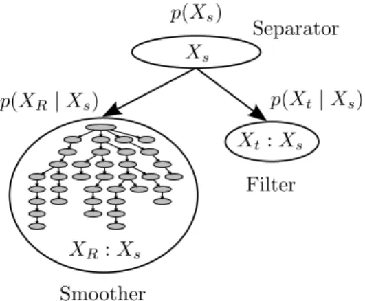
Figure 1. Smoother and filter combined in a single optimization problem and represented as a Bayes tree. A separator is selected so as to enable parallel computations.
Simultaneous localization and mapping (SLAM) algorithms in robotics perform a similar state estimation task, but addi-tionally can include loop closure constraints at higher latency. The goal of SLAM is to find the optimal position and attitude estimate at each time interval given all of the available measurements. This requires solving a large, nonlinear least-squares problem, with solutions ranging from off-line batch approaches to recent innovations in incremental smoothing. In addition to improved estimates from nonlinear optimization, SLAM systems also take advantage of identified loops in the robot’s trajectory. These loop closures serve to both correct drift accumulated over the loop and bound the estimation uncertainty. While SLAM systems make use of vehicle nav-igation data within the optimization, the improved results of the SLAM solution are rarely fed back to the navigation filter as an aiding source.
In this paper we propose concurrent filtering and smoothing by viewing the speed navigation filter and the high-latency localization smoother as operations performed within a single graphical model known as a Bayes tree. With this representation it becomes clear that the filtering and smoothing operations may be performed independently while still achiev-ing an optimal state estimate at any time. This approach has been tested on simulated aerial vehicle data with navigation estimates being performed at 100Hz. In all cases the filter operated in real time with the final trajectory approaching the optimal trajectory estimate obtained from a full nonlinear batch optimization.
In what follows, Section II reviews related work that solves the tracking and mapping problem through the use of parallel processes. In Section III we review filtering and smoothing and present the key insight to our approach. Section IV describes the graphical model known as a Bayes tree used to represent the full smoothing problem. The specifics of the proposed concurrent filtering and mapping algorithm are given in Section V. Experimental results evaluating our algorithm on synthetic data are presented in Section VI. Finally conclusions and future work are discussed in Section VII.
II. RELATEDWORK
Many filtering-based solutions to the navigation problem exist that are capable of integrating multiple sensors [2]. Examples include GPS-aided [6] and vision-aided [20, 33, 8] inertial navigation. A recent overview of filtering and related methods to multi-sensor fusion can be found in [27]. In addition to the extended Kalman filter (EKF) and variants such as the unscented Kalman filter, solutions also include fixed-lag smoothing [19]. While delayed and/or out-of-sequence data can also be handled by filters [1, 26, 32], fixed-lag smoothing additionally allows re-linearization [25, 17]. However, filter-ing and fixed-lag smoothfilter-ing based navigation solutions are not able to probabilistically include loop closure constraints derived from camera, laser or sonar data; the most useful loop closures reach far back in time to states that are no longer represented by such methods.
Integration of loop closures requires keeping past states in the estimation and can be solved efficiently by smoothing. Originally in the context of the simultaneous localization and mapping (SLAM) problem, a set of landmarks has been estimated using the EKF [28, 29, 22]. However, the EKF solution quickly becomes expensive because the covariance matrix is dense, and the number of entries grows quadratically in the size of the state. It has been recognized that the dense correlations are caused by elimination of the trajectory [5, 3]. The problem can be overcome by keeping past robot poses in the estimation instead of just the most recent one, which is typically referred to as full SLAM or view-based SLAM. Such a solution was first proposed by Lu and Milios [16] and further developed by many researchers including [30, 5, 3, 18, 13]. Even though the state space becomes larger by including the trajectory, the problem structure remains sparse and can be solved very efficiently by smoothing [3]. Here we use an incremental solution to smoothing by Kaess et al. [10].
View-based SLAM solutions typically only retain a sparse set of previous states and summarize the remaining informa-tion. For high rate inertial data, summarization is typically done by a separate filter, often performed on an inertial measurement unit (IMU). Marginalization is used to remove unneeded poses and landmarks, good examples are given in [7, 12]. And finally, the so-called pose graph formulation omits explicit estimation of landmark locations, and instead integrates relative constraints between pairs of poses. Despite all the reductions in complexity, smoothing solutions are not
constant time when closing large loops and are therefore not directly suitable for navigation purposes.
Similar to our work, filtering and smoothing has been combined in a single optimization by Eustice et al. [5]. Their exactly sparse delayed state filter retains select states as part of the state estimate, allowing loop closures to be incorporated. The most recent state is updated in filter form, allowing integration of sensor data at 10Hz. Their key realization was the sparsity of the information form, and an approximate solution was used to provide real-time updates. Our solution instead provides an exact smoothing solution incorporating large numbers of states, while being able to process high rate sensor data on the filtering side with minimum delay.
A navigation solution requires constant processing time, while loop closures require at least linear time in the size of the loop; hence parallelization is needed. Klein and Murray [11] proposed parallel tracking and mapping (PTAM) of a single camera, where localization and map updates are performed in parallel. This differs from the navigation problem because filtering is replaced by repeated re-localization of the camera with respect to the current map. Still, the key idea of per-forming slower map updates in parallel is directly applicable to navigation. In addition, the bundle adjustment (BA) [31] used to optimize the map is mathematically equivalent to the smoothing solution deployed in our work: the only difference is the specific structure of the problem, which is more sparse in our navigation case. The same parallelization is also used in more recent dense solutions such as dense tracking and mapping by Newcombe et al. [24] and KinectFusion by Newcombe et al. [23]. However, while this separation into relocalization and mapping works well for tracking a camera, it does not allow probabilistic integration of inertial sensor data as achieved by our work.
Probably the closest work in navigation is the dual-layer estimator by Mourikis and Roumeliotis [21] for combined camera and inertial estimation that uses an EKF for fast processing and BA for limiting linearization errors. However, they do not sufficiently explain how the BA result is fed back into the filter, in particular how consistent feedback is performed without rolling back the filter. Rolling back measurements is made unnecessary in our formulation, which casts the concurrent filtering and smoothing processes as a single, parallelized optimization problem.
Our novel solution combines filtering and smoothing within a single estimation framework, while formulating it in such a way that both are performed concurrently. Hence the filter operates at constant time when integrating new sensor data, while updates from the slower smoother are integrated on the fly once they become available.
III. FILTERING ANDSMOOTHING
Existing navigation systems typically integrate the sensor data using a filtering approach [6]. Most common are EKF based solutions, in particular the error state EKF. Such filtering methods provide a constant time solution for estimating the most recent state xt, and can therefore process high frame
rate sensor data, in particular from inertial sensors, with minimal delay. The best estimate ˆXtis given by the maximum
likelihood solution ˆ
Xt= arg max Xt
p (Xt| Z) . (1)
In addition to the current state estimate xt, the set Xt may
include landmarks or select previous states that are required to provide a better estimate of xt. New states Xt0are constantly
being added, while the previous states are integrated out p (Xt0 | Z) =
ˆ
Xt
p (Xt, Xt0| Z) . (2)
Better estimates of the current state can be obtained by integrating loop closure constraints that provide relative mea-surements to earlier states. Such loop closure constraints can be generated, for example, by appearance-based methods operating on key image frames, or from laser scan matching and 3D model alignment approaches.
However, loop closure constraints cannot simply be added into the filtering formulation, which only estimates the most recent pose. Instead, the earlier state referred to by the loop closure must be part of the estimation problem. Instead of integrating out all variables, as in filtering solutions, a typical solution is to retain select variables. Variables to retain can be selected by regular sub-sampling of the states, or by selecting states that correspond to key frames of visual odometry systems. The resulting estimation problem grows over time and cannot be solved efficiently in a filtering framework. Instead, efficient smoothing solutions have been presented that exploit the sparsity of the underlying problem structure. The optimal smoothing solution ˆX over all states is given by the maximum likelihood
ˆ
X = arg max
X
p (X | Z) . (3)
Unfortunately, a straightforward smoothing solution is not suitable to high speed navigation. New states Xt0are constantly
being added, yielding a growing number of states that need to be estimated
p (X0| Z) = p (X, Xt0 | Z) . (4)
In contrast to filtering over a single state, even incremen-tal smoothing [10] over a growing number of states with occasional inclusion of loop closure constraints generally is not a constant time operation. The navigation system needs to provide the best estimate at any time, incorporating new measurements at sensor frame rate.
Key Insight
The key insight underlying our work is that a smoothing solution can be parallelized, allowing the problem to be split into a high speed navigation component and a higher latency loop closure component. The key idea is to select a suitable separator to allow running of the smoother and filter in parallel. Over the last years, progress has been made in parallelizing estimation algorithms by partitioning the state space in an
(a) Factor graph
(b) Chordal Bayes net
(c) Bayes tree
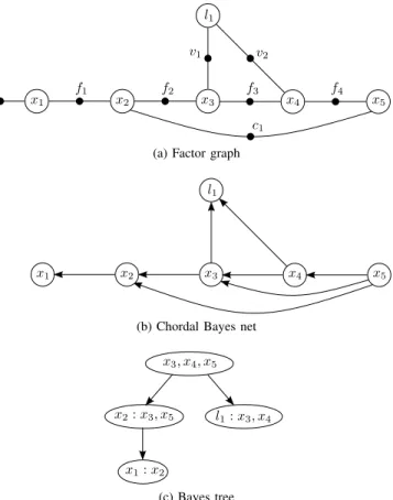
Figure 2. (a) An example factor graph is shown with five state variables xiconnected by inertial factors fi. The factor c1 represents a loop closure.
A landmark l1 with two visual measurements vk is also shown. (b) The
equivalent chordal Bayes net for the variable ordering: l1, x1, x2, x3, x4,
x5. (c) The equivalent Bayes tree constructed by identifying cliques.
appropriate manner, e.g. Dellaert et al. [4]. Partitioning al-gorithms such as nested dissection [15] are well known. The goal of such methods is to find separators that split the problem into multiple parts that can be solved in parallel.
Here we introduce a single separator near the most recent state to separate the low latency filter component from the loop closure calculations in the smoother. We denote the separator by Xs, and the sparse set of older states by XR. In the
smoothing formulation of (3), the posterior factors into three components
p (X | Z) = q (X) = q (XR| Xs) q (Xs) q (Xt| Xs) . (5)
For brevity we omitted the measurement Z from the notation by defining q (·) := p (· | Z). The factors from left to right represent the smoother, the separator and the filter. Both, the smoother and the filter, can be solved in parallel (because they are independent given the separator), and can then be joined at the separator.
In the next section we discuss how we address the naviga-tion problem using this formulanaviga-tion as a single optimizanaviga-tion problem, initially ignoring real-time constraints. In the follow-ing section we then provide the concurrent solution for real-time operation, where multiple filter updates are performed during a single iteration of the smoother.
IV. SMOOTHINGSOLUTION
Here we provide a smoothing solution to the navigation problem using the recently introduced Bayes tree [9, 10]. While this approach does not provide a constant time solution, it forms the basis for the incremental and parallel computation described in Section V.
We use a factor graph [14] to represent the smoothing navigation problem as a graphical model; an example is shown in Figure 2a. A factor graph is a bipartite graph G = (F , X, E ) with two node types: factor nodes fi ∈ F and variable
nodes xj ∈ X. An edge eij ∈ E is present if and only if
factor fi involves variable xj. The factor graph G defines the
factorization of a function f (X) as a product of factors fi
f (X) =Y
i
fi(Xi) , (6)
where Xi = {xj|eij∈ E} is the set of variables xj adjacent
to factor fi.
In the navigation context, a sensor measurement is repre-sented as a factor affecting select variables. For example, a GPS measurement affects a single state variable, while an inertial measurement affects two or more states, depending on how bias estimation is implemented. A generative model
zi= hi(Xi) + νi (7)
predicts a measurement ziusing a function hi(Xi) with added
measurement noise νi. The difference between the prediction
ˆ
zi = hi(Xi) and the actual measurement zi is represented by
the factor
fi(Xi) = di[hi(Xi) − zi] (8)
for some cost function di. If the underlying noise process is
Gaussian with covariance Σ, the distance metric is simply the Mahalanobis distance d(r) = krk2Σ, but more general functions such as robust estimators can also be accommodated. We use variable elimination on the factor graph as a basis for efficient inference [10]. To eliminate a variable xj from
the factor graph, we first form the joint density fjoint(xj, Sj)
of all adjacent factors, where the separator Sj consists of all
involved variables except for xj. Applying the chain rule,
we then obtain a new factor fnew(Sj) and a conditional
p (xj| Sj). For a given variable ordering, all variables are
eliminated from the factor graph, and the remaining condi-tionals form a chordal Bayes net
p (X) =Y
j
p (xj| Sj) . (9)
An example is shown in Figure 2b. The elimination order affects the graph structure and therefore also the computational complexity. Good orderings are provided by efficient heuristics such as minimum degree.
The solution is obtained from the Bayes tree, which is created by identifying cliques in the chordal Bayes net. An example is shown in Figure 2c. Cliques are found by traversing the graph in reverse elimination order. A node is added to its parent’s clique if they are fully connected, otherwise a new
clique is started. The resulting cliques are denoted by Fk : Sk,
where Fkare the frontal variables, resulting in the factorization
p (X) =Y
k
p (Fk| Sk) . (10)
Inference in the Bayes tree proceeds top-down: The root has no dependencies and can directly be solved; the solution is passed on to its children, which in turn can then be solved.
V. CONCURRENTFILTERING ANDSMOOTHING
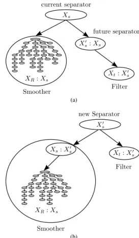
(a)
(b)
Figure 3. (a) Filter operation marginalizes out unused variables, but select key states are retained for the smoother to allow for loop closings. Key states that are no longer needed by the filter eventually form cliques along a chain between the current separator and the filter. (b) The separator is advanced by a simple change in the variable elimination ordering so that the original separator becomes a part of the smoother.
Here we view the full smoothing problem with the particular factorization of (5), so that smoothing over past states is decou-pled from filtering on current states. The posterior p (X | Z) in (5) is equivalent to a Bayes tree with the separator as root, as shown in Figure 3. Because the separator is chosen to be the root of the Bayes tree, it is always eliminated last, which indicates a point of synchronization. As a consequence, the filter and smoother may run in parallel, with the filter typically performing multiple steps during one smoother iteration. Com-putations are independent except for at the separator, where they are fused.
A. Filter
The filter has three goals: 1) Integrate new factors as they become available. 2) Keep the complexity constant by removing unused states. 3) Leave some key states behind for integration into the smoother. Here we discuss how these goals are reached.
Integrating a new factor into the existing Bayes tree is fast because the integration is independent of the smoother and only affects the filter and separator cliques. Let us assume the new factor to be added is fn(Xn) with Xn ⊆ Xt;
this is true for sensor measurements but does not include loop closures, which instead are directly integrated into the smoother as described later. By definition, the new factor directly affects the filter clique Xt. Changing a clique also
affects all ancestors, which can easily be seen from the elimination algorithm passing information upwards towards the root, which is eliminated last. Consequently, the separator clique Xsalso has to be recalculated. By the same
argumenta-tion, the smoother cliques in XRare eliminated independently
up to the separator and are therefore unaffected by the new information integrated into the filter.
Integrating a new factor requires temporarily converting the affected cliques back into a factor graph [10]. While converting the factor graph to a Bayes tree requires elimination, the opposite direction is trivial. Each clique X : Y can directly be written as a factor f (X, Y ), and the new factor is simply added. The resulting factor graph is converted back to a Bayes tree as usual, and the smoother clique is re-added without change. Solving of the filter state also does not involve the smoother, and is therefore only dependent on the size of the filter.
To keep the filter operating in constant time, it needs to remove intermediate states that are no longer needed. States have to be kept in the filter states Xt as long as
they might be referred to by future factors. Once no new sensor measurements can directly affect a state, we call that state inactive. Removal of inactive states is done during the integration of new states: By choosing a suitable variable ordering the inactive states are eliminated first. Marginalization over inactive states corresponds to simply dropping their conditionals from the chordal Bayes net, before the Bayes tree is created by clique finding.
For integration into the smoother, select key states are retained even after they become inactive in the filter to allow future loop closings. The key states are selected to provide a sparse set of summarized poses that support integration of loop closures in the smoother to (nearly) arbitrary states in the past. One simple strategy is to retain key poses at fixed time intervals, and more advanced approaches additionally take into account the usefulness of a state, for example in terms of visual saliency. The variable ordering is modified so as to insert these states between the filter and separator states, which eventually leads to the formation of additional cliques as shown in Figure 3a. We will see in Section V-C how these cliques eventually end up in the smoother.
B. Smoother
The main goal of the smoother is to integrate loop closure constraints. One type of loop closure constraint is a relative one between two states, such as arising from laser-scan match-ing or derived from visual constraints. Another type arises from multiple observations of an unknown landmark over time. We ignore known landmarks here, which can be treated in the same way as GPS measurements: they can directly be integrated into the filter as unary constraints.
Loop closures can only be introduced in the smoother. Introducing loop closures in the filter that connect to older variables in the smoother would circumvent the separator, therefore destroying the conditional independence of filter and smoother. If one of the variables referred to by a loop closure constraint is still part of the filter, that state is marked as a key state, and the loop closure is delayed until that key state has migrated to the smoother. That delay is not problematic for the navigation solution because loop closures are typically calculated in the background and are only available with some delay. Their main goal is to constrain long term drift, while the filter produces very accurate results locally.
While the smoother could simply perform batch optimiza-tion, it is cheaper to update the existing solution with the newly added information using the iSAM2 algorithm [10]. The smoother updates the conditional p (XR| Xs) and the
separator p (Xs), while the filter p (Xt| Xs) is conditionally
independent and does not change. C. Synchronization
So far we have discussed how the filter and the smoother work independently from each other; we will now focus on the concurrent operation that is needed in practice to provide a navigation solution with only a small constant delay.
Concurrent operation requires synchronization between the independently running filter and smoother. Synchronization happens after each iteration of the smoother. The filter runs multiple iterations by the time a single iteration of the smoother finishes. To achieve constant delay in the filter, the filter can never wait for the smoother. Hence, upon finishing an iteration, the smoother waits for the filter to finish its current update.
At the time of synchronization, the orphaned subtree of the filter is merged back into the updated tree of the smoother. However, the original separator has changed independently in both the smoother and the filter. Our solution is to incorporate from the filter only the change with respect to the original separator—exactly the information the filter would add had it been run in sequence with the smoother instead of in parallel. The synchronization is constant time because only the root is changed. After synchronization, filter and smoother again form a consistent Bayes tree, and the filter can immediately continue with the integration of new information.
The last missing piece is how to move inactive key states from the filter to the smoother; this is done during synchro-nization by a modification of the variable ordering. After the root nodes are merged, the separator and the cliques consisting
−500 0 500 1000 1500 −1000 −500 0 500 −50 0 50 100 150 200 North (m) East (m) Down (m) Trajectory Landmarks
Figure 4. A visualization of the simulated ground truth trajectory of an aerial vehicle. Ground-based landmarks are observed from a downward-facing stereo camera.
of key states are re-eliminated with a variable ordering that changes the separator closer to the filter and therefore transfers the previous separator and potential intermediate states into the smoother. This advancing of the separator is visualized in Figure 3.
VI. RESULTS
To test the concurrent smoothing and mapping system, sensor measurements from an aerial vehicle simulator were generated. The simulator models vehicle dynamics as well as the effects induced from moving along the Earth’s surface, such as non-constant gravity, non-constant craft rate, and Cori-olis effects. The simulated aerial vehicle traverses a survey-type trajectory, circling around a section of terrain several times. An illustration of the simulated trajectory is shown in Figure 4. The simulation system produces ground truth IMU measurements at 100Hz and low-frequency visual odometry from ground landmarks at 0.5 Hz. Additionally, a sparse set of loop closures were identified within the visual data. A total of 22 such constraints were generated at five different locations corresponding to trajectory crossings.
All measurements were corrupted with white noise before being given to the estimation system, IMU terms additionally with a constant bias. Bias terms were drawn from a zero-mean Gaussian distribution with a standard deviation of σ = 10 mg for the accelerometers and σ = 10 deg/hr for the gyroscopes. The noise terms were drawn from a zero-mean Gaussian dis-tribution with σ = 100 µg/√Hz and σ = 0.001 deg/√hr for the accelerometers and gyroscopes. Zero-mean Gaussian noise with σ = 0.5 pixels was added to all visual measurements.
Using these simulated sensors, an inertial strapdown system has been implemented inside of the filter. This strapdown system integrates the IMU measurements to create estimates of velocity, position, and orientation. While the IMU integration is very accurate over short time periods, measurement errors
can quickly accumulate, resulting is significant estimation drift over time. To counter this drift, additional sensor are used to aid the inertial strapdown at lower frequencies. Global measurements, such as GPS or magnetometer readings, are typical aiding sources, though the use of vision as an aiding source has become common. For this simulated example, the low-frequency visual odometry measurements serve the purpose of strapdown aiding. Though this significantly limits the state estimate drift, visual odometry measurements them-selves provide only relative pose information. Consequently, significant state estimation errors can accumulate over long time horizons.
The filtering estimates can be improved by incorporating the longer-term loop closure constraints into the smoother. For the concurrent filtering and smoothing example, the filter has been designed to send the summarized states associated with the visual odometry frames to the smoother. When a loop closure constraint is identified, it is sent to the smoother. Once the smoother has recalculated the trajectory using this new constraint, the filter and smoother are synchronized, as described in Section V-C. While the smoother is recalculating, the filter continues to process the IMU measurements and produce updated state estimates in real-time.
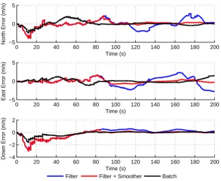
Figures 5-7 show a comparison of the estimation errors produced from the filter only, the concurrent filtering and smoothing system, and a full batch optimization. The filtering only solution uses the inertial strapdown with the visual odometry aiding; no loop closures are incorporated. This rep-resents a typical navigation filtering solution. The concurrent filtering and smoothing results use the inertial strapdown with the visual odometry aiding on the filtering side, while loop closure constraints are provided to the smoother. Unlike the filtering solution, long-term loop closures at arbitrary positions along the trajectory can be incorporated without affecting the time of the filter. Finally, a series of full batch optimizations have been performed. Each state estimate within the batch trajectory results from a full, nonlinear optimization of all measurements up to the current time. This trajectory captures the best possible state estimate at each time instant using only measurements available up to that time.
The concurrent filtering and smoothing system is able to correct the estimated trajectory using loop closure constraints, approaching the performance of full batch optimization. How-ever, unlike batch approaches or even recent incremental smoothing techniques, the update frequency of the filtering portion of the concurrent system is unaffected by the incor-poration of these large loop closures. Real-time performance is achieved on the filtering side, with state updates from the sensor measurements and synchronization updates from the smoother requiring less than 1ms on average, well below the 10ms between sequential IMU readings. Timing was performed on a single core of an Intel i7-2600 processor with a 3.40GHz clock rate and 16GB of RAM memory. Figure 8 displays histograms of the actual calculation times for the constant-time filter updates and the filter-smoother synchronization times for the simulated example.
0 20 40 60 80 100 120 140 160 180 200 −100 −50 0 50 Time (s) North Error (m) 0 20 40 60 80 100 120 140 160 180 200 −100 0 100 200 Time (s) East Error (m) 0 20 40 60 80 100 120 140 160 180 200 −50 0 50 Time (s) Down Error (m)
Filter Filter + Smoother Batch
Figure 5. Position estimation errors produced by a filter only, the concurrent filtering and smoother, and a full batch optimization.
0 20 40 60 80 100 120 140 160 180 200 −5 0 5 Time (s) North Error (m/s) 0 20 40 60 80 100 120 140 160 180 200 −5 0 5 Time (s) East Error (m/s) 0 20 40 60 80 100 120 140 160 180 200 −4 −2 0 2 Time (s) Down Error (m/s)
Filter Filter + Smoother Batch
Figure 6. Velocity estimation errors produced by a filter, the concurrent filter and smoother, and a full batch optimization.
0 20 40 60 80 100 120 140 160 180 200 −0.02 0 0.02 0.04 Time (s)
Roll Error (rad)
0 20 40 60 80 100 120 140 160 180 200
−0.05 0 0.05
Time (s)
Pitch Error (rad)
0 20 40 60 80 100 120 140 160 180 200
−0.1 0 0.1
Time (s)
Yaw Error (rad)
Filter Filter + Smoother Batch
Figure 7. Rotation estimation errors produced by a filter, the concurrent filter and smoother, and a full batch optimization.
0.4 0.6 0.8 1 1.2 0 2000 4000 6000 8000 10000 12000 14000
Filter Update Time (ms)
0.4 0.6 0.8 1 0 5 10 15 20 25 30 Synchronization Time (ms)
Figure 8. Histograms of the filter update delay and the filter-smoother synchronization delay for the simulated example. All times are well below the 10ms between sequential IMU updates.
VII. CONCLUSION
We presented a novel navigation algorithm that combines constant time filtering with the loop closing capabilities of full trajectory smoothing. Using the Bayes tree and choosing a suitable separator allows us to parallelize these complimentary algorithms. Smoothing is performed in an efficient incremental fashion using iSAM2. After each iteration, synchronization with the filter takes place, allowing information from loop closures to be rapidly incorporated into the real-time fil-tering solution. The validity of the proposed approach was demonstrated in a simulated environment that includes IMU, visual odometry and camera-based loop closure constraints, and compared to both a filter and a full batch optimization.
While the computational complexity of the filter is constant in time, the smoother grows unboundedly, which can be addressed in a number of ways. One solution is to drop old states, which is similar to fixed-lag smoothing methods, but allows for optimization and loop closures over much larger time windows because of the parallelization. Another approach that has been proposed in the SLAM community is to sparsify the trajectory over time.
While not addressed here, multi-rate and out-of-sequence measurements can be handled similar to fixed-lag smoothing approaches in the literature [32], by keeping multiple recent states in the filter instead of just the most recent one.
Marginalization combines linearized factors in the filter, making it difficult to perform relinearization in the smoother. Solutions exist in the presence of only pairwise constraints, such as the lifting of factors described in [12]. We expect that similar methods can be developed for more complicated factors such as IMU with bias estimates. Ongoing research is investigating the integration of the concurrent smoothing and filtering algorithm with a generic plug-and-play navigation architecture that incorporates IMU measurements in real-time.
ACKNOWLEDGMENTS
We would like to thank Rakesh Kumar and Supun Sama-rasekera at Sarnoff/SRI International for their support and valuable discussions. This work was supported by the all source positioning and navigation (ASPN) program of the Air Force Research Laboratory (AFRL) under contract FA8650-11-C-7137. The views expressed in this work have not been endorsed by the sponsors.
REFERENCES
[1] Y. Bar-Shalom, “Update with out-of-sequence measurements in tracking: exact solution ,” IEEE Trans. Aerosp. Electron. Syst., vol. 38, pp. 769–777, 2002.
[2] Y. Bar-Shalom and X. Li, Multitarget-multisensor tracking: principles and techniques. YBS Publishing, 1995.
[3] F. Dellaert and M. Kaess, “Square Root SAM: Simultaneous lo-calization and mapping via square root information smoothing,” Intl. J. of Robotics Research, vol. 25, no. 12, pp. 1181–1203, Dec 2006.
[4] F. Dellaert, A. Kipp, and P. Krauthausen, “A multifrontal QR factorization approach to distributed inference applied to multi-robot localization and mapping,” in Proc. 22nd
AAAI National Conference on AI, Pittsburgh, PA, 2005, pp. 1261–1266. [5] R. Eustice, H. Singh, and J. Leonard, “Exactly sparse
delayed-state filters for view-based SLAM,” IEEE Trans. Robotics, vol. 22, no. 6, pp. 1100–1114, Dec 2006.
[6] J. Farrell, Aided Navigation: GPS with High Rate Sensors. McGraw-Hill, 2008.
[7] J. Folkesson and H. Christensen, “Graphical SLAM – a self-correcting map,” in IEEE Intl. Conf. on Robotics and Automa-tion (ICRA), vol. 1, 2004, pp. 383–390.
[8] E. Jones and S. Soatto, “Visual-inertial navigation, mapping and localization: A scalable real-time causal approach,” Intl. J. of Robotics Research, vol. 30, no. 4, Apr 2011.
[9] M. Kaess, V. Ila, R. Roberts, and F. Dellaert, “The Bayes tree: An algorithmic foundation for probabilistic robot mapping,” in Intl. Workshop on the Algorithmic Foundations of Robotics, Dec 2010.
[10] M. Kaess, H. Johannsson, R. Roberts, V. Ila, J. Leonard, and F. Dellaert, “iSAM2: Incremental smoothing and mapping using the Bayes tree,” Intl. J. of Robotics Research, vol. 31, pp. 217– 236, Feb 2012.
[11] G. Klein and D. Murray, “Parallel tracking and mapping for small AR workspaces,” in IEEE and ACM Intl. Sym. on Mixed and Augmented Reality (ISMAR), Nara, Japan, Nov 2007, pp. 225–234.
[12] K. Konolige and M. Agrawal, “FrameSLAM: from bundle adjustment to realtime visual mapping,” IEEE Trans. Robotics, vol. 24, no. 5, pp. 1066–1077, 2008.
[13] K. Konolige, G. Grisetti, R. Kuemmerle, W. Burgard, L. Ben-son, and R. Vincent, “Efficient sparse pose adjustment for 2D mapping,” in IEEE/RSJ Intl. Conf. on Intelligent Robots and Systems (IROS), Taipei, Taiwan, Oct 2010, pp. 22–29. [14] F. Kschischang, B. Frey, and H.-A. Loeliger, “Factor graphs
and the sum-product algorithm,” IEEE Trans. Inform. Theory, vol. 47, no. 2, February 2001.
[15] R. Lipton, D. Rose, and R. Tarjan, “Generalized nested dissec-tion,” SIAM Journal on Applied Mathematics, vol. 16, no. 2, pp. 346–358, 1979.
[16] F. Lu and E. Milios, “Globally consistent range scan alignment for environment mapping,” Autonomous Robots, pp. 333–349, Apr 1997.
[17] T. Lupton and S. Sukkarieh, “Visual-inertial-aided navigation for high-dynamic motion in built environments without initial
conditions,” IEEE Trans. Robotics, vol. 28, no. 1, pp. 61–76, Feb 2012.
[18] I. Mahon, S. Williams, O. Pizarro, and M. Johnson-Roberson, “Efficient view-based SLAM using visual loop closures,” IEEE Trans. Robotics, vol. 24, no. 5, pp. 1002–1014, Oct 2008. [19] P. Maybeck, Stochastic Models, Estimation and Control. New
York: Academic Press, 1979, vol. 1.
[20] A. Mourikis and S. Roumeliotis, “A multi-state constraint Kalman filter for vision-aided inertial navigation,” in IEEE Intl. Conf. on Robotics and Automation (ICRA), April 2007, pp. 3565–3572.
[21] ——, “A dual-layer estimator architecture for long-term local-ization,” in Proc. of the Workshop on Visual Localization for Mobile Platforms at CVPR, Anchorage, Alaska, June 2008. [22] P. Moutarlier and R. Chatila, “An experimental system for
incremental environment modelling by an autonomous mobile robot.” in Experimental Robotics I, The First International Symposium, Montréal, Canada, June 19-21, 1989, 1989, pp. 327–346.
[23] R. Newcombe, A. Davison, S. Izadi, P. Kohli, O. Hilliges, J. Shotton, D. Molyneaux, S. Hodges, D. Kim, and A. Fitzgib-bon, “KinectFusion: Real-time dense surface mapping and tracking,” in IEEE and ACM Intl. Sym. on Mixed and Augmented Reality (ISMAR), Basel, Switzerland, Oct 2011, pp. 127–136. [24] R. Newcombe, S. Lovegrove, and A. Davison, “DTAM: Dense
tracking and mapping in real-time,” in Intl. Conf. on Computer Vision (ICCV), Barcelona, Spain, Nov 2011, pp. 2320–2327. [25] A. Ranganathan, M. Kaess, and F. Dellaert, “Fast 3D pose
estimation with out-of-sequence measurements,” in IEEE/RSJ Intl. Conf. on Intelligent Robots and Systems (IROS), San Diego, CA, Oct 2007, pp. 2486–2493.
[26] X. Shen, E. Son, Y. Zhu, and Y. Luo, “Globally optimal dis-tributed Kalman fusion with local out-of-sequence-measurement updates,” IEEE Transactions on Automatic Control, vol. 54, no. 8, pp. 1928–1934, Aug 2009.
[27] D. Smith and S. Singh, “Approaches to multisensor data fusion in target tracking: A survey,” IEEE Transactions on Knowledge and Data Engineering, vol. 18, no. 12, p. 1696, Dec 2006. [28] R. Smith, M. Self, and P. Cheeseman, “A stochastic map for
uncertain spatial relationships,” in Proc. of the Intl. Symp. of Robotics Research (ISRR), 1988, pp. 467–474.
[29] ——, “Estimating uncertain spatial relationships in Robotics,” in Autonomous Robot Vehicles, I. Cox and G. Wilfong, Eds. Springer-Verlag, 1990, pp. 167–193.
[30] S. Thrun, W. Burgard, and D. Fox, Probabilistic Robotics. The MIT press, Cambridge, MA, 2005.
[31] B. Triggs, P. McLauchlan, R. Hartley, and A. Fitzgibbon, “Bun-dle adjustment – a modern synthesis,” in Vision Algorithms: Theory and Practice, ser. LNCS, W. Triggs, A. Zisserman, and R. Szeliski, Eds. Springer Verlag, 2000, vol. 1883, pp. 298– 372.
[32] S. Zahng and Y. Bar-Shalom, “Optimal update with multiple out-of-sequence measurements,” in Proc. of the SPIE, Signal Processing, Sensor Fusion, and Target Recognition XX, May 2011.
[33] Z. Zhu, T. Oskiper, S. Samarasekera, R. Kumar, and H. Sawh-ney, “Ten-fold improvement in visual odometry using landmark matching,” in Intl. Conf. on Computer Vision (ICCV), Oct 2007.