HAL Id: hal-01234361
https://hal.archives-ouvertes.fr/hal-01234361
Submitted on 26 Nov 2015
HAL is a multi-disciplinary open access
archive for the deposit and dissemination of
sci-entific research documents, whether they are
pub-lished or not. The documents may come from
teaching and research institutions in France or
abroad, or from public or private research centers.
L’archive ouverte pluridisciplinaire HAL, est
destinée au dépôt et à la diffusion de documents
scientifiques de niveau recherche, publiés ou non,
émanant des établissements d’enseignement et de
recherche français ou étrangers, des laboratoires
publics ou privés.
Multi-Armed Bandits for Adaptive Constraint
Propagation
Amine Balafrej, Christian Bessière, Anastasia Paparrizou
To cite this version:
Amine Balafrej, Christian Bessière, Anastasia Paparrizou. Multi-Armed Bandits for Adaptive
Con-straint Propagation. IJCAI: International Joint Conference on Artificial Intelligence, Jul 2015, Buenos
Aires, Argentina. pp.290-296. �hal-01234361�
Multi-Armed Bandits for Adaptive Constraint Propagation
∗Amine Balafrej
TASC (INRIA/CNRS), Mines Nantes
Nantes, France
[email protected]
Christian Bessiere
CNRS, U. Montpellier
Montpellier, France
[email protected]
Anastasia Paparrizou
CNRS, U. Montpellier
Montpellier, France
[email protected]
Abstract
Adaptive constraint propagation has recently re-ceived a great attention. It allows a constraint solver to exploit various levels of propagation dur-ing search, and in many cases it shows better per-formance than static/predefined. The crucial point is to make adaptive constraint propagation auto-matic, so that no expert knowledge or parameter specification is required. In this work, we pro-pose a simple learning technique, based on multi-armed bandits, that allows to automatically select among several levels of propagation during search. Our technique enables the combination of any num-ber of levels of propagation whereas existing tech-niques are only defined for pairs. An experimen-tal evaluation demonstrates that the proposed tech-nique results in a more efficient and stable solver.
1
Introduction
Constraint propagation is an essential component for effi-ciently solving constraint satisfaction problems (CSPs). Due to its ability to reduce the search space, constraint propaga-tion is considered as the reason for the success and spread of Constraint Programming (CP) in solving many large-scale, real-world problems. Since the early 70’s, CP research has provided a wide range of effective, either general-purpose or specialized propagation techniques. Despite this big variety, CP solvers need a expert user to tune the solver so that it becomes more efficient. In addition, solvers are constraint oriented, in the sense that they associate a specialized prop-agation for each type of constraint. On the other hand, the drawback of this design, is that they overlook the general pic-ture of the problem (i.e., structural dependencies, constraint intersections) as well as the internal operations that occur dur-ing search. For example, in many cases, propagation effects indicate a need for changing the ordering in variable selection (e.g., domain wipeouts in dom/wdeg heuristic [Boussemart et al., 2004]).
This work aims at developing a simple framework that can learn the right combination of propagation levels during solv-ing (online). It is based on a light learnsolv-ing technique, called
∗
This work was supported by the EU under the project ”Inductive Constraint Programming”, contract FP7 FET-Open 284715.
multi-armed bandits (MAB), that was inspired by the slot ma-chines in casinos and the problem that a gambler has to decide which machines to play, in which order and how many times to play each one. Each machine, after being used, returns a re-ward from a distribution specific to that machine. The goal is to maximize the sum of rewards obtained through a sequence of plays [Gittins, 1989].
We use a MAB model to select the right level of propaga-tion (also called level of consistency) to enforce at each node during the exploration of the search tree. We specify a simple reward function and the upper confidence bound (UCB) to es-timate the best arm, namely the best consistency to apply. An experimental evaluation on various benchmark classes shows that the proposed framework, though being simple and pre-liminary, results in a more efficient and stable solver. We provide a clear evidence that the proposed adaptive technique is able to construct the right combination of the available con-sistency algorithms of a solver. It can be much more efficient than any level of consistency alone. The MAB framework as proposed here does not require any training or information from preprocessing and can improve its decision vigorously during search.
2
Related Work
Although CP community has provided a wide range of effi-cient propagation techniques, standard solvers do not adjust the propagation level depending on the characteristics of the problem. They either preselect the propagator or use costs and other measures to order the various propagation tech-niques. In [Schulte and Stuckey, 2008], some state-of-the-art methods are presented to order propagation techniques in well known solvers (e.g., Gecode, Choco).
There has been a significant amount of work on adaptive solving through the use of machine learning (ML) methods, either with a training phase or without. The goal of the learning process is to automatically select or adapt the search strategy, so that the performance of the system is improved. There are two main approaches that have been studied. In the first case, a specific strategy (e.g., a search algorithm or a specific solver) is selected automatically among an ar-ray of available strategies, either for a whole class of prob-lems or for a specific instance. Such methods, called portfo-lios, perform the learning phase offline, on a training set of instances. Portfolios have been initially proposed for SAT
(e.g., SATzilla [Xu et al., 2008]) and then for CSPs (e.g., CPHydra [O’Mahony et al., 2008], Proteus [Hurley et al., 2014]). In the second case, a new strategy can be synthe-sized (e.g., a combination of search algorithm and heuris-tics) through the use of ML [Epstein and Petrovic, 2007; Xu et al., 2009]. The learning phase is again performed as a preprocessing. On the contrary, in [Loth et al., 2013], multi-armed bandits are exploited to select online (i.e., with-out training phase) which node of a Monte Carlo Tree Search (MCTS) to extend. In that paper, the Bandit Search for Con-straint Programming (BaSCoP) algorithm adapts MCTS to the CSP search to explore the most promising regions accord-ing to a specified reward function.
There has been little research on learning strategies for constraint propagation. In [Epstein et al., 2005], ML is used to construct a static method for the pre-selection between For-ward Checking and Arc Consistency. The work in [Kotthoff et al., 2010] evaluates ensemble classification for selecting an appropriate propagator for the alldifferent constraint. But this is again done in a static way prior to search.
Recent papers have shown an increasing interest for adapt-ing the propagation level through the use of heuristic meth-ods. The initial approach, appeared in [Stergiou, 2008], showed many advantages in favor of heuristics. They are both inexpensive to apply and dynamic, based on the actual effects of propagation during search (i.e., domain wipeouts (DWOs), value deletions). This approach was later improved by a more general model for n-ary constraints that does not require any parameter tuning [Paparrizou and Stergiou, 2012]. This di-rection of research has led to the parameterized local consis-tencyapproach for adjusting the level of consistency depend-ing on a stability parameter over values [Balafrej et al., 2013; Woodward et al., 2014]. Parameterized local consistencies choose to enforce either arc consistency or a stronger local consistency on a value depending on whether the stability of the value is above or below a given threshold. Interestingly, they propose ways to dynamically adapt the parameter, and thus the level of local consistency, during search. In [Balafrej et al., 2014], the number of times variables are processed for singleton tests on their values is adapted during search. The learning process is based on measuring a stagnation in the amount of pruned values.
Thus, we have on the one hand the use of ML tech-niques that are heavy to be applied online and can be mainly used prior to search (static). Hence the actual effect during search is ignored. In addition, the vast majority of works in this direction were proposed for adapting the variable order-ing heuristics, not for adaptorder-ing the propagation level durorder-ing search. On the other hand, we have heuristics methods to automatically adapt consistency during search, but heuristics are only defined for two levels of consistency (i.e., a weak and a strong one). This limits their applicability.
The technique we propose in this paper fills the gap in the literature by proposing a ML approach for selecting automati-cally and dynamiautomati-cally among any number of propagation lev-els, without the need for training.
3
Background
A constraint network is defined as a set of n variables X = {x1, ..., xn}, a set of domains D = {D(x1), ..., D(xn)}, and
a set of e constraints C = {c1, ..., ce}. Each constraint ck
is defined by a pair (var(ck), sol(ck)), where var(ck) is an
ordered subset of X , and sol(ck) is a set of combinations of
values (tuples) satisfying ck.
The technique presented in this paper is totally generic in the sense that it can be used with any set of local consis-tencies. In our experiments, we use arc consistency (AC), max restricted path consistency (maxRPC), and partition one arc consistency (POAC). We give the necessary background to understand them. As maxRPC is defined for binary con-straints only, we simplify the notations by considering that all constraints are binary. A binary constraint between xiand
xj will be denoted by cij, and Γ(xi) will denote the set of
variables xjinvolved in a constraint with xi.
A value vj ∈ D(xj) is called an arc consistent (AC)
sup-port for vi ∈ D(xi) on cij iff (vi, vj) ∈ sol(cij). A value
vi ∈ D(xi) is arc consistent (AC) if and only if for all
xj ∈ Γ(xi) vi has an AC support on cij. A network is arc
consistent if all the values of all its variables are arc consis-tent. We denote by AC(N ) the network obtained by enforc-ing arc consistency on N .
A value vj ∈ D(xj) is a max restricted path consistent
(maxRPC)support for vi∈ D(xi) on cijif and only if it is an
AC support and the tuple (vi, vj) can be extended to any third
variable xkwhile satisfying cikand cjk. A value vi∈ D(xi)
is maxRPC iff for all xj ∈ Γ(xi) vi has a maxRPC support
vj∈ D(xj) on cij. A network is maxRPC if all the values of
all its variables are maxRPC.
Given a constraint network N = (X , D, C), a value vi ∈
D(xi) is partition-one-AC (POAC) iff AC(N ∪ {xi = vi})
does not have empty domains, and ∀j ∈ 1..n, j 6= i, ∃vj ∈
D(xj) such that vi ∈ AC(N ∪ {xj = vj}). A network is
POAC if all the values of all its variables are POAC.
4
Multi-Armed Bandits for Adaptive
Constraint Propagation
We describe a simple framework for adaptive propagation based on Multi-Armed Bandits (MAB). The successive se-lection of a consistency level during search is a sequential de-cision problem and as such, it can be represented as a multi-armed or k-multi-armed (for k different consistencies) bandit prob-lem. One needs to select amongst k consistencies to enforce in order to maximize the cumulative reward by selecting each time the best one. Initially, such a choice is taken under uncer-tainty, since the underlying reward distributions are unknown. Later in the process, potential rewards are estimated based on past observations. The more the search tree grows, the more knowledge we acquire and the better decisions we make.
The critical question that needs to be addressed in ban-dit problems is related to the tradeoff between ”exploitation” of the arm with the greatest expected reward (based on the knowledge already acquired) and ”exploration” of other, cur-rently sub-optimal arms to further increase knowledge about them and which may become superior in the future. This is
related to the exploitation vs. exploration dilemma in rein-forcement learning.
4.1
The multi-armed bandit model
We use the multi-armed bandit problem to learn what is the appropriate level of consistency to enforce during solving a CSP. We call MAB selector the ML component that decides a level of consistency to use. We can have such a selector for each constraint, for each variable, or, more coarsely, for each level of the search tree. The selector is based on a model defined over:
• A set of k arms {LC1, . . . , LCk}. Each arm corresponds
to an algorithm that enforces a specific level of local con-sistency.
• A set of rewards Ri(j) ∈ R, 1 ≤ i ≤ k, j ≥ 1, where
Ri(j) is the reward delivered when an arm LCihas been
chosen at time j.
The reward function can be any measure that reflects the performance or a criterion that indicates the appropriate arm. The performance can be either positive (e.g., values removed) or negative (e.g., CPU time).
In MAB models, we must define a policy to choose the next arm based on the sequence of previous trials. It is important not to discard an arm forever to ensure that any arm that could become later optimal is not omitted in favor of other currently sub-optimal arms. As a result, it is useful to know the upper confidence bound(UCB) that any given arm will be optimal. Since the model cannot always make the best decision, its expected loss or regret is considered after m times. Auer et al. [Auer and Cesa-Bianchi, 2002], propose a simple UCB policy that has an expected logarithmic growth of regret uni-formly over m (not just asymptotically) without any prior knowledge regarding the reward distributions. Their policy, called UCB1, selects the arm i that maximizes:
ρ(i) = ¯Ri+
r 2 ln m mi
(1) where ¯Ri is the mean of the past rewards of the i arm, mi
is the number of times arm i was selected and m is the cur-rent number of all trials. The reward term ¯Riencourages the
exploitation of local consistencies with higher-rewards, while
theq2 ln mm
i term promotes the exploration of the less selected
local consistencies.
The literature contains more elaborated versions of multi-armed bandits where additional parameters allow to insist more on exploration or exploitation depending on the context. As one of our goal is to assess the simplicity of this direction of research, we use the most basic regret policy defined in equation 1, where no parameter tuning is required.
4.2
A MAB selector for adapting consistency
online
When designing a MAB selector we have to define the reward function and to decide the granularity at which the MAB op-erates. Concerning the granularity, there exist various natural ways to attach MAB selectors to a CP solver. We could de-cide to attach a MAB selector per variable in the network,
per constraint, etc. Depending on the place where a MAB selector is attached, the most natural parameters used for the reward function may change.
In this preliminary work, we follow an observation made by Debruyne. In [Debruyne, 1998], he observed that chang-ing the level of consistency with the depth in the search tree can improve search significantly. By depth, we mean the number of variables assigned.1 In his work, Debruyne was manually tuning the solver to change the level of consistency from AC to maxRPC or maxRPC to AC at predefined depths depending on the class of problems, based on his own experi-ence. We then decided to define a MAB model where we have a MAB selector at each depth in the search tree. Our goal is to show that the MAB selectors will learn by themselves which level of local consistency to use at which depth.
Once the places to attach MAB selectors is decided, we have to define the reward function. We chose to define a re-ward function that takes into account the actual CPU time needed to explore the subtree rooted at this depth once the decision of which local consistency to use has been taken by the MAB selector of the given depth.
For each depth in the search tree we have a separate MAB selector, with its own time parameter j. We denote by Ti(m)
the CPU time needed to enforce LCiat the mth visit of a node
at the given depth plus the time to explore the subtree rooted there. (Ti(m) is not defined if this is not LCithat has been
chosen at time m.) The reward Ri(j) is computed based on
the performance of LCiat time j compared to performance
of all consistencies at previous visits at this depth. Ri(j) = 1 −
Ti(j)
maxi=1..k,m=1..j(Ti(m))
(2) Formula 2 is normalized so that Ri(j) ∈ [0, 1]. Indeed,
re-member that ρ in Formula 1 computes the sum of rewards. The backtrack search algorithm that uses this MAB model calls the MAB selector of a given depth h each time it in-stantiates a variable at depth h in the search tree. The search algorithm progressively builds a search tree and applies a lo-cal consistency LCi at depth h guided by results of previous
choices at the same depth.
These are the steps that the algorithm follows after each variable assignment x ← a:
1. We call the MAB selector of the depth at which x ← a occurs.
2. We select the LCithat maximizes ρ(i).
3. We store the current time startT ime[depth] of the ma-chine.
4. LCiis executed on that node.
5. When backtracking to that node, we read the current time endT ime of the machine and we update the re-ward Ri(j). Ti(j), which was defined as the sum of
the CPU time required to enforce LCi after the
as-signment of x plus the CPU time required to explore the resulting subtree is simply obtained by endT ime − startT ime[depth].
1
In 2-way branching, x = a is considered as an assignment whereas the refutation x 6= a is not.
160 180 200 220 240 260 280 300 500 1000 2000 3000 3600 # So lv ed In st an ce s CPU(s) AC AC-maxRPC AC-POAC AC-maxRPC-POAC maxRPC POAC 50 100 150 0 1 3 5
Figure 1: Number of instances solved per algorithm when the time allowed increases (cactus plot).
5
Experimental Evaluation
We ran experiments on problem classes from real world ap-plications and classes following a regular pattern involving a random generation (REAL and PATT in www.cril.univ-artois.fr/˜lecoutre/benchmarks.html). The algorithms were implemented with a CP solver written in Java and tested on an 2.8 GHz Intel Xeon processor and 16 GB RAM. A cut-off of 3,600 seconds was set for all algorithms and all instances. We used the dom/deg heuristic for variable ordering and lexico-graphic value ordering. We used three levels of consistency: AC (AC2001 [Bessiere et al., 2005]), maxRPC (maxRPC3 [Balafoutis et al., 2011]), and POAC (POAC1 [Balafrej et al., 2014]). For AC2001 and maxRPC3 we used their residual versions ([Lecoutre and Hemery, 2007]) to avoid maintain-ing AC and maxRPC supports durmaintain-ing search. From these three consistencies we built six solving methods: Three of them maintain a single local consistency during the whole search (AC, maxRPC or POAC). The three others are adap-tive methods using a MAB selector to decide which local consistency to apply among {AC, maxRPC}, {AC, POAC} and {AC, maxRPC, POAC}, respectively denoted by AC-maxRPC, AC-POAC and AC-maxRPC-POAC.
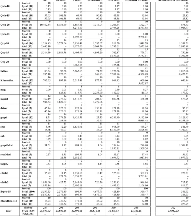
Table 1 (except last column) shows the results of the six solving methods where the adaptive ones use a MAB selec-tor for each depth in the search tree and a reward function based on CPU time as described in Section 4.2. Comparing these six methods on the instances solved by all of them, we observe that overall, adaptive methods are faster than meth-ods maintaining a single consistency. This is especially true on difficult problems. The row ’Total’ (last row of the ta-ble) shows that all adaptive methods have a total sum of CPU time smaller than the CPU time of methods maintain-ing a smaintain-ingle consistency. The adaptive method usmaintain-ing the three consistencies (AC-maxRPC-POAC) is the fastest. The total number of solved instances confirms this behavior as adap-tive methods including a strong consistency LC solve more instances than those maintaining LC alone. Once more, AC-maxRPC-POAC is the best, solving 309 instances among the
313 tested.
When looking at the results in more details, we observe that in a few cases, when one of the local consistencies behaves significantly worse than the others (such as POAC in graph), the MABs including it are penalized. The reason is that UCB forces the MABs to select this bad consistency for exploration purposes. It takes some time to learn not to select it.
In the last column of Table 1, we report the results of an experiment done to assess the learning capabilities of our MAB selectors. The solver uses the three consistencies AC, maxRPC, and POAC, but instead of using a MAB selector to select the right consistency to apply at a node, it selects one consistency randomly. Thanks to the use of three consisten-cies, this baseline algorithm has a good behavior. It is better than any single consistency and also better than MAB selec-tors with only two consistencies. But when the MAB also uses three consistencies, it has a significantly better behavior (faster and solving more instances).
In Figure 1, we report the cactus plot of the number of instances solved per method while the time limit increases. What we see on the zoom on the first seconds of time is that AC is the one that solves the more instances in less than 5 seconds and POAC the less. When the time limit is be-tween 5 seconds and approximately 200 seconds, maxRPC is the one that solves more instances while AC deteriorates. Among the methods maintaining a single consistency, POAC is the one that solves the fewest instances until we reach a time limit of 500 seconds. After 500 seconds, AC becomes the worst among all and it remains the worst until the cut-off of 3600 seconds. Concerning the adaptive methods, AC-maxRPC is second best in the zone where AC-maxRPC is the best (5-200 seconds). But as time increases, POAC and AC-maxRPC-POAC solve more instances than the other methods, AC-maxRPC-POAC being the clear winner by solving more instances than all others from 200 seconds until the cutoff.
The important information that this cactus plot gives us, is that, on very hard instances, the adaptive methods are never worse than any consistency they include (e.g., AC-maxRPC
Table 1: Sum of CPU times (in sec.) and #solved instances per class and per algorithm.
AC maxRPC POAC AC-maxRPC AC-POAC AC-maxRPC-POAC AC-maxRPC-POAC(rand)
#solved 10 10 10 10 10 10 10 Qwh-10 by all (10) 0.13 0.90 1.70 0.98 1.17 1.10 0.88 total (10) 0.13 0.90 1.70 0.98 1.17 1.10 0.88 #solved 10 10 10 10 10 10 10 Qwh-15 by all (10) 57.05 101.58 64.99 90.43 43.38 43.04 23.82 total (10) 57.05 101.58 64.99 90.43 43.38 43.04 23.82 #solved 9 9 10 9 10 10 10 Qwh-20 by all (9) 10,462.54 8,154.69 1,887.81 7,316.04 1,206.34 1,322.77 875.43 total (10) – – 5,216.10 – 2,498.25 2,747.93 1,908.37 #solved 0 0 1 0 0 1 0 Qwh-25 by all (0) 0.00 0.00 0.00 0.00 0.00 0.00 0.00 total (1) – – 1,097.18 – – 2,756.81 – #solved 15 14 15 15 15 15 15 Qcp-10 by all (14) 1,214.43 3,771.64 3,136.48 1,535.67 919.30 1,011.78 1,351.31 total (15) 2,446.10 – 6,672.00 3,064.59 1,792.01 2,472.14 2,985.48 #solved 11 11 14 12 15 15 15 Qcp-15 by all (11) 5,314.59 5,984.78 1,405.99 4,895.20 762.87 779.71 750.86 total (15) – – – – 5,559.25 5,752.51 5,302.56 #solved 0 0 1 0 1 1 1 Qcp-20 by all (0) 0.00 0.00 0.00 0.00 0.00 0.00 0.00 total (1) – – 3,463.16 – 425.46 2,085.15 2,259.63 #solved 21 21 18 21 21 21 21 fullins by all (18) 83.64 93.56 5,662.63 74.39 1,722.36 941.24 1,815.86 total (21) 295.18 273.65 – 248.83 7,707.86 4,536.69 8,472.53 #solved 16 16 15 16 16 17 16 K-insertion by all (15) 763.65 993.19 2,015.41 875.71 969.95 660.66 646.94 total (17) – – – – – 5,475.87 – #solved 4 8 8 8 8 8 8 mug by all (4) 0.00 0.01 0.80 0.01 0.39 0.27 0.24 total (8) – 523.43 115.77 2,233.90 142.03 115.73 177.32 #solved 12 12 11 12 11 11 11 myciel by all (11) 167.19 273.72 1,815.73 204.77 607.56 486.10 573.75 total (12) 944.54 1,622.67 – 1,279.06 – – – #solved 7 7 7 7 7 7 7 driver by all (7) 45.74 225.61 125.14 130.11 121.18 98.94 93.83 total (7) 45.74 225.61 125.14 130.11 121.18 98.94 93.83 #solved 14 14 12 14 13 14 14 graph by all (12) 1.31 274.28 9,420.51 23.33 6,289.40 3,192.09 3,121.45 total (14) 1.99 288.66 – 32.63 – 6,019.48 6,358.70 #solved 11 11 9 11 11 11 11 scen by all (9) 3.46 12.20 1,630.91 9.91 915.99 469.27 541.49 total (11) 18.36 47.07 – 36.99 6,157.79 3,595.95 4,709.37 #solved 9 9 9 9 9 9 9 sub by all (9) 0.29 0.02 0.40 0.02 0.42 0.02 0.05 total (9) 0.29 0.02 0.40 0.02 0.42 0.02 0.05 #solved 5 6 9 6 10 10 8 graphMod by all (5) 31.51 1.12 984.18 1.04 538.94 296.68 1,508.19 total (10) – – – – 1,830.11 1,300.54 – #solved 3 9 9 8 9 9 9 scenMod by all (3) 0.37 1.31 193.59 1.04 83.67 57.48 56.93 total (9) – 21.58 3,182.17 – 1,694.72 1,017.94 1,979.75 #solved 8 7 2 7 2 7 5 fapp02 by all (2) 0.63 1.05 0.63 1.44 0.58 1.58 0.81 total (10) – – – – – – – #solved 5 6 6 5 5 6 5 e0ddr1 by all (5) 35.92 11.15 1,038.62 10.47 525.02 302.13 272.21 total (6) – 271.36 3,958.70 – – 3,783.61 – #solved 7 6 7 6 7 7 7 e0ddr2 by all (6) 1,859.00 425.52 2,143.04 720.36 1,256.85 996.04 717.12 total (7) 1,859.14 – 2,492.11 – 1,493.95 1,106.86 819.77 #solved 100 100 100 100 100 100 100 Bqwh-18 by all (100) 5,539.53 2,376.40 696.34 4,677.91 423.80 360.47 386.93 total (100) 5,539.53 2,376.40 696.34 4,677.91 423.80 360.47 386.93 #solved 10 10 10 10 10 10 10 BlackHole-4-4 by all (10) 18.94 337.52 371.11 48.02 46.34 82.80 273.99 total (10) 18.94 337.52 371.11 48.02 46.34 82.80 273.99 #solved 287 296 293 296 300 309 302 Total by all (270) 25,599.92 23,040.25 32,596.01 20,616.86 16,435.51 11,104.16 13,012.12 Total (313) – – – – – – –
is close to maxRPC and better than AC) and they can even be superior to any consistency they include (e.g., AC-POAC solves constantly more instances than AC or POAC). This means that given an instance to solve, they not only under-stand which consistency is the best overall, but they benefit from the temporary superiority of another consistency.
We also ran Adaptive POAC [Balafrej et al., 2014] on the same classes. Adaptive POAC is generally faster than MABs on easy instances. On hard instances, Adaptive POAC is far slower than MABs containing POAC: it only solves 296 in-stances overall, that is, more than single consistencies and AC-maxRPC, but less than AC-POAC, AC-maxRPC-POAC, and AC-maxRPC-POAC(rand).
6
Discussion
Simplicity of use and low computation cost are good rea-sons to choose multi-armed bandits for adapting consistency during search. Low computation cost is an essential prop-erty for an online technique. Another reason is that suc-cessive choices of a consistency at a given depth yield re-wards that are independent. This ensures that there is no hidden correlation that a MAB selector could not learn (as MABs only learn independent rewards). In a setting where we would learn sequences of choices of local consistencies on a sequence of successive depths, a Q-learning framework would probably be more relevant [Sutton and Barto, 1998; Xu et al., 2009].
The MAB model as defined in equations 1 and 2 has originally been proposed for stationary arms, that is, arms for which the reward received when playing an arm follows a probability distribution that remains unchanged along the plays. Under this condition, UCB1 ensures that the average regret converges to zero with probability 1, that is, UCB1 en-sures that the optimal arm is played exponentially more often than any other arm. In our setting, however, we cannot guar-antee that arms are stationary because the reward of a local consistency may change as search progresses. Several ver-sions of UCB have been proposed to deal with environments that change over time. However, it is recognized that the ba-sic UCB has low probability to show a worst-case behavior when applied to such changing environments [Fialho et al., 2010]. In addition, versions of UCB that deal with chang-ing environments require some parameter tunchang-ing, such as the decay factor or the length of time window. As observed in [Fialho et al., 2010], a bad configuration of the parameters can produce too much forgetting when the environment does not change as fast as expected. For these reasons, in this first attempt to exploit MAB in adaptive propagation, we chose to remain on the simple version of UCB where there is no parameter to tune before use.
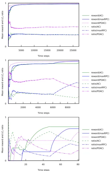
To illustrate this ability of UCB to adapt despite dynamic environment, we focus on the internal behavior of our MABs. Figure 2 displays the internal behavior of the MAB selector AC-maxRPC-POAC at several depths (77, 104, 155) when solving the instance 3-insertion-4-3. As time increases, the values of the mean reward ¯Ri and the ratio of calls to each
consistency are plotted. (The ratio is the number of times LCi
was selected divided by total number of times the selector 0 1 5000 10000 15000 20000 25000 M ea n rew a rd a n d LC i r at io Time steps reward(AC) reward(maxRPC) reward(POAC) ratio(AC) ratio(maxRPC) ratio(POAC) 0 1 2000 4000 6000 8000 M ea n rew a rd a n d LC i r at io Time steps reward(AC) reward(maxRPC) reward(POAC) ratio(AC) ratio(maxRPC) ratio(POAC) 0 1 20 40 60 80 M ea n rew a rd a n d LC i r at io Time steps reward(AC) reward(maxRPC) reward(POAC) ratio(AC) ratio(maxRPC) ratio(POAC)
Figure 2: Instance 3-insertion-4-3: Mean rewards and ratios of each consistency at depths 77 (top), 104 (middle), and 155 (bottom).
was called.) On all three graphs we observe that MAB selects more frequently the local consistency with the highest mean reward. On the top graph we see that at depth 77, POAC is learned as the best and is then chosen the most often. On the middle graph we see that in the begining, POAC is preferred to AC and maxRPC because its mean reward is the highest. After 6000 time steps, maxRPC suddenly starts increasing its reward resulting in being quickly promoted, as the steep inclination of its ratio curve shows. This both illustrates that rewards are non stationary and that our simple UCB is able to detect it. Finally, on the bottom graph we see that at depth 155 (close to the leaves) things are less clear but AC tends to be the preferred one, confirming an observation made in [Debruyne, 1998].
Figure 2 shows that MAB learns what is the most effi-cient consistency to enforce at a given time during search. AC-maxRPC-POAC solved this instance in 1, 661 seconds, POAC in 4, 602 seconds and both AC and maxRPC failed to solve it in 4 hours. The adaptive technique was able to be faster than the best consistency alone (here POAC),
be-cause it is able to enforce the right consistency at the right node during search. MAB selectors can construct the right combination of the available propagation levels of a solver, adapted to each instance, without any preprocessing knowl-edge or other information prior to search. These first results show the potentiality of a CP solver that is able to exploit any algorithm that it has in its arsenal without having the knowl-edge of when/where to use it. This is another step in the di-rection of an autonomous solver.
7
Conclusion
In this paper, we have introduced a simple framework for adaptive constraint propagation based on multi-armed ban-dits learning. The proposed framework allows the automatic selection of the right propagation technique among several, overcoming the strong limitation of previous works. Due to its light learning mechanism, our framework can be ap-plied dynamically, considering the effects of propagation dur-ing search. The experiments on various benchmark classes showed that the proposed framework increases the efficiency and robustness of a CP solver.
Acknowledgments
We would like to thank Nadjib Lazaar for his help on multi-armed bandits.
References
[Auer and Cesa-Bianchi, 2002] P. Auer and P. Cesa-Bianchi, N.and Fischer. Finite-time analysis of the multiarmed ban-dit problem. Machine Learning, 47(2-3):235–256, 2002. [Balafoutis et al., 2011] T. Balafoutis, A. Paparrizou,
K. Stergiou, and T. Walsh. New algorithms for max restricted path consistency. Constraints, 16(4):372–406, 2011.
[Balafrej et al., 2013] A. Balafrej, C. Bessiere, R. Coletta, and E. Bouyakhf. Adaptive parameterized consistency. In Proceedings of CP’13, pages 143–158, 2013.
[Balafrej et al., 2014] A. Balafrej, C. Bessiere, E. Bouyakhf, and G. Trombettoni. Adaptive singleton-based consisten-cies. In Proceedings of AAAI’14, pages 2601–2607, 2014. [Bessiere et al., 2005] C. Bessiere, J.C. R´egin, R. Yap, and Y. Zhang. An Optimal Coarse-grained Arc Consistency Algorithm. Artificial Intelligence, 165(2):165–185, 2005. [Boussemart et al., 2004] F. Boussemart, F. Hemery,
C. Lecoutre, and L. Sais. Boosting systematic search by weighting constraints. In Proceedings of ECAI’04, pages 146–150, 2004.
[Debruyne, 1998] R. Debruyne. Etude des consistances lo-cales pour les probl`emes de satisfaction de contraintes de grande taille. PhD thesis, LIRMM-Universit´e de Mont-pellier II, December 1998.
[Epstein and Petrovic, 2007] S. Epstein and S. Petrovic. Learning to Solve Constraint Problems. In ICAPS-07 Workshop on Planning and Learning, 2007.
[Epstein et al., 2005] S. Epstein, E. Freuder, R. Wallace, and X. Li. Learning propagation policies. In Proceedings of the 2nd International Workshop on Constraint Propaga-tion and ImplementaPropaga-tion, pages 1–15, 2005.
[Fialho et al., 2010] A. Fialho, L. Da Costa, M. Schoenauer, and M. Sebag. Analyzing bandit-based adaptive opera-tor selection mechanisms. Ann. Math. Artif. Intell., 60(1-2):25–64, 2010.
[Gittins, 1989] J. C. Gittins. Multi-Armed Bandit Allocation Indices, volume 10. John Wiley and Sons, 1989.
[Hurley et al., 2014] H. Hurley, L. Kotthoff, Y. Malitsky, and B. O’Sullivan. Proteus: A hierarchical portfolio of solvers and transformations. In Proceedings of CPAIOR’2014, pages 301–317, 2014.
[Kotthoff et al., 2010] L. Kotthoff, I. Miguel, and P. Nightin-gale. Ensemble Classification for Constraint Solver Con-figuration. In Proceedings of CP’10, pages 321–329, 2010.
[Lecoutre and Hemery, 2007] C. Lecoutre and F. Hemery. A study of residual supports in arc consistency. In Proceed-ings of IJCAI’07, pages 125–130, 2007.
[Loth et al., 2013] M. Loth, M. Sebag, Y. Hamadi, and M. Schoenauer. Bandit-based search for constraint pro-gramming. In Proceedings of CP’13, pages 464–480, 2013.
[O’Mahony et al., 2008] E. O’Mahony, E. Hebrard, A. Hol-land, C. Nugent, and B. O’Sullivan. Using case-based rea-soning in an algorithm portfolio for constraint solving. In Proceedings of AICS’10, 2008.
[Paparrizou and Stergiou, 2012] A. Paparrizou and K. Ster-giou. Evaluating simple fully automated heuristics for adaptive constraint propagation. In Proceedings of IEEE-ICTAI’12, pages 880–885, 2012.
[Schulte and Stuckey, 2008] C. Schulte and P.J. Stuckey. Ef-ficient Constraint Propagation Engines. ACM Trans. Pro-gram. Lang. Syst., 31(1):1–43, 2008.
[Stergiou, 2008] K. Stergiou. Heuristics for Dynamically Adapting Propagation. In Proceedings of ECAI’08, pages 485–489, 2008.
[Sutton and Barto, 1998] R. S. Sutton and A. G. Barto. Rein-forcement learning: An introduction. IEEE Transactions on Neural Networks, 9(5):1054–1054, 1998.
[Woodward et al., 2014] R.J. Woodward, A. Schneider, B.Y. Choueiry, and C. Bessiere. Adaptive parameterized con-sistency for non-binary csps by counting supports. In Pro-ceedings of CP’14, pages 755–764, 2014.
[Xu et al., 2008] L. Xu, F. Hutter, H. H. Hoos, and K. Leyton-Brown. Satzilla: Portfolio-based algorithm se-lection for SAT. J. Artif. Intell. Res. (JAIR), 32:565–606, 2008.
[Xu et al., 2009] Y. Xu, D. Stern, and H. Samulowitz. Learn-ing Adaptation to solve Constraint Satisfaction Problems. In Proceedings of LION, 2009.