Space charge measurement in solid dielectrics by the pulsed electro-acoustic technique

HAL Id: hal-00019789

https://hal.archives-ouvertes.fr/hal-00019789

HAL is a multi-disciplinary open access archive for the deposit and dissemination of sci-entific research documents, whether they are pub-lished or not. The documents may come from teaching and research institutions in France or abroad, or from public or private research centers.

L’archive ouverte pluridisciplinaire HAL, est destinée au dépôt et à la diffusion de documents scientifiques de niveau recherche, publiés ou non, émanant des établissements d’enseignement et de recherche français ou étrangers, des laboratoires publics ou privés.

Space charge measurement in solid dielectrics by the

pulsed electro-acoustic technique

Olivier Gallot-Lavallée, G. Teyssedre

To cite this version:

Olivier Gallot-Lavallée, G. Teyssedre. Space charge measurement in solid dielectrics by the pulsed electro-acoustic technique. 2006. �hal-00019789�

Space charge measurement in solid dielectrics by the pulsed electro-acoustic technique

1

Université Paul Sabatier, Laboratoire de Génie Electrique de Toulouse, 118, route de Narbonne, Toulouse, 31062, France

Abstract: Born in 1985, the PEA technique consists in detecting acoustic waves generated by space charges when they are subjected to an impulse of electric field. Its principle is relatively simple to understand and its use is very flexible. Compared to other techniques as LIPP (Laser Induced Pressure Pulse) method and TSM (Thermal Step Method), the PEA technique is the only one being not based on the relative displacement of the space charge in respect to the electrodes. We show here how consistent information on space charge can be extracted from a simple physical equation and we discuss with the help of a simple modeling the effect of numerical processes such as Gaussian filter.

INTRODUCTION

Until recently, charge storage effect was only probed using techniques capable of yielding information about integral quantities of charges such as thermally-stimulated discharge studies. During the 1980s, a new class of techniques was developed with the ability of disclosing differential data such as the charge distribution along the thickness direction. In most of these methods, a displacement of charges is imposed relatively to the measuring electrodes in a capacitor where the dielectric is placed between two metallic electrodes [1,2,3,4]. The influence charge on the electrodes is thus modified and this variation is measured in the external circuit. This signal is transformed into a voltage variation across the sample terminals in case of the measurement being performed in open circuit or into a current variation in the case of a short-circuit measurement. The charge displacement is induced by an external perturbation applied to the sample in such a way as to modify its transversal dimension in a non-uniform manner, this last condition being necessary to obtain an electrical response from the deformation of a charged material. In addition, the form and the evolution of the perturbation as a function of time must be known during the measurements.

In practice, the relative movement of the charge with respect to the electrodes can be controlled by a non-uniform expansion of the medium induced by a temperature variation on one of the sample sides (methods known as thermal [5,6,7] or by the generation of a pressure wave (methods known as acoustic [8,9]. These methods can take different names depending on the type of stimulation

applied, thermal or acoustic, and its shape. Finally, there is a third method known as the Pulsed Electro-Acoustic technique [10,11] based on a different principle. Here, a voltage pulse is applied to the sample to provide stimulation. The induced electric field produces on each existing charge a Coulomb force. Acoustic waves are thus engendered by the exchange of momentum between the electrical charges, bound to the atoms of the dielectric, and the medium. These waves are then detected by a piezoelectric sensor and recorded as function of time to provide the basis for the reconstruction of a one-dimensional distribution of the space charge bulk density.

In the 1990s, these techniques matured and were routinely used in labs and industrial sites [12]. Among them, pressure wave propagation (acoustic) and thermal methods became popular in Europe and North-America [13,14,15,16], whereas the pulsed electro acoustic technique was preferred in Japan [17,18]. In spite of the fact that the situation is currently undergoing a change [19,20,21] the PEA method is still less well-known in Europe. The objective of this communication is to provide a simple physical way to comprehend this technique. We discuss notably the consequences of approximations and numerical errors due to e.g. Gaussian filter effect.

DESCRIPTION OF THE PULSED ELECTRO-ACOUSTIC METHOD

Measurement principle

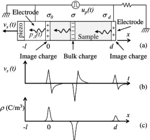
The PEA measurement principle is given in Fig. 1. Let us consider a sample having a thickness d presenting a layer of negative charge σ at a depth x. This layer induces on the electrodes the charges σd

and σ0 by total influence so that:

σ σ σ σ . 0 . d d x and d x d − = − = (1)

Application of a pulsed voltage up(t) induces a

transient displacement of the space charges around their positions along the x-axis under Coulomb effect. Thus elementary pressure waves pΔ(t), issued

from each charged zone, with amplitude proportional to the local charge density propagates inside the sample with the speed of sound. Under the influence of these pressure variations, the piezoelectric sensor delivers a voltage vs(t) which is

characteristic of the pressures encountered. The charge distribution inside the sample becomes accessible by acoustic signal treatment. The quantification of the measurements passes by a referencing procedure whose description will follow. up(t) vs(t) -l 0 d x σ0 σ σd -l 0 d x ρ(C/m3₎ p_Δ(t) t vs(t) vs(t) Sample Electrode pie zo Electrode Bulk charge

Image charge Image charge

(a) (b) (c) up(t) vs(t) -l 0 d x σ0 σ σd -l 0 d x ρ(C/m3₎ p_Δ(t) t vs(t) vs(t) Sample Electrode pie zo Electrode Bulk charge

Image charge Image charge

(a)

(b)

(c)

Figure 1: Principle of the PEA method. (a) Charged regions give rise to acoustic waves under the effect of a pulsed field. (b) As a consequence the piezoelectric sensor delivers a voltage vs(t). (c) An

appropriate signal treatment then gives the spatial distribution of image and internal charges.

Theoretical analysis

Main measurement Let us consider a sample with a volumic charge distribution ρ as shown in Fig. 2 and divide it in a set of rigid charged layers of thickness Δx and homogeneous charge density. The force fΔ(x,t) representing the dynamical component

of the force exerted on each layer of the x-axis due to the coupling of the electric field pulse e(t) with the charge is thus expressed as:

) ( . . ). ( ) , (xt x xSet f_Δ =ρ Δ (2) Rigid charged volume e q. fr= r f e f .dρ e f volume∫ = r r f_Δ e Δx S (m2₎ e f_Δ f_Δ xr Rigid charged volume e q. fr= r f e f .dρ e f volume∫ = r r f_Δ e Δx S (m2₎ e f_Δ f_Δ xr

Figure 2: Model for the equation set up

The pressure waves, obtained dividing f by the surface S of the electrode, reaches the piezoelectric

detector without changing shape with the following hypothesis: the acoustic wave propagates in a homogeneous and perfectly elastic medium, i.e. attenuation and acoustic dispersion factors are nil in Fourier space [22,23,24]. The delay between wave production and detection is directly dependent on the speed of sound characteristic of each material traversed, being designated by vp for the sample and

ve for the electrode of thickness l adjacent to the

piezoelectric sensor. The pressure seen by the detector is as follows: x x v x v l t e t x p p e Δ − − = Δ( , ) ( ).ρ( ). (3)

The pressure exerted on the sensor by the entire set of elementary layers is obtained thereafter by the summation:

∫

∫

Note that the electric field e is nil outside the dielectric, i.e. ∀ x ∉ [0,d].

Setting τ =x /v_p and ρ(x)=ρ(τ.vp)=r(τ) gives:

∫

The form of Equ. 5 being that of a convolution, it can be simplified by the application of Fourier transform: ] . 2 exp[ ). ( ). ( . )] ( F[ ) ( e p v l i E R v t p Pν = = ν ν − πν (6)

As for the piezoelectric sensor, its output vs(t) and

its input p(t) can be expressed by a convolution law such as, in the Fourier space:

) ( ). ( ) (ν Hν Pν Vs = (7)

where H(ν) is the characteristic transfer function of the piezoelectric sensor, encompassing the entire set of the amplifier and the waveguide, from the practical point of view.

At this stage of argument, one unknown remains to be eliminated, H(ν), for obtaining R(ν)…

Reference measurement The referencing procedure illustrated in Fig. 3 has the role to eliminate the unknown H(ν) which is the characteristic transfer function of the piezoelectric sensor and related electronics. For that we consider a sample free from charges to which a constant

voltage U is applied. The surface density of the charge (capacitive charge) on the electrodes is then:

1 1 1 . d U ε σ = (8) up (t) vs1 (t) -l 0 d1 x U p1Δ(t) t vs1 (t) d1 /vp l /ve up (t) vs1 (t) -l 0 d1 x U p1Δ(t) t vs1 (t) d1 /vp l /ve

Figure 3: Principle of the reference measurement. The reference signal is that produced by the capacitive charges located on the electrode adjacent to the piezoelectric sensor ( solid line).

Here and in what follows, the index 1 refers to calibration data.

With the hypothesis that the capacitive charges due to the pulsed field e are negligible compared to all others, the pressure thus created by the electrode nearest to the sensor is expressed as:

) ( . ) ( 1 1 e v l t e t p =σ − ] . 2 exp[ ). ( . ) ( )] ( F[ _{1 1 1} e v l i E P t p = ν =σ ν − πν ⇒ (9)

Piezoelectric conversion properties being always the same, we have:

) ν ( P ). ν ( H ) ν ( Vs₁ = ₁ (10)

from which H(ν) is extracted.

Result after calibration Combining Equ. (6, 7, 9 and 10), we obtain the expression of F[ρ(x)] as:

) ( ) ( . ) ( 1 1 ν ν σ ν Vs Vs v R p = (11)

Now ρ(x) is obtained by the inverse transform of Fourier, such as:

⎥ ⎥ ⎦ ⎤ ⎢ ⎢ ⎣ ⎡ = = − − ) ( ) ( . . . F )] ( [ F ) ( 1 1 1 1 1 ν ν ε ν ρ s s p V V d v U R x (12)

As such, the charge profile determination passes by two measurements: the first gives us vs(t) to be

converted to Vs(ν) by Fourier transform; the second

(reference) gives us vs1(t) to be converted to Vs1(ν).

Experimental errors

According to Maeno [24] and Alison [23], three types of error can be identified, in addition to acoustic dispersion and/or multiple scattering of the acoustic waves : i/ a random error due to noise within the experimental system, which is eliminated with signal averaging carried out in PEA method; ii/ systematic errors in the signal calibration parameters, e.g. sample thickness d1, applied

voltage U, velocity vp and dielectric permittivity ε1

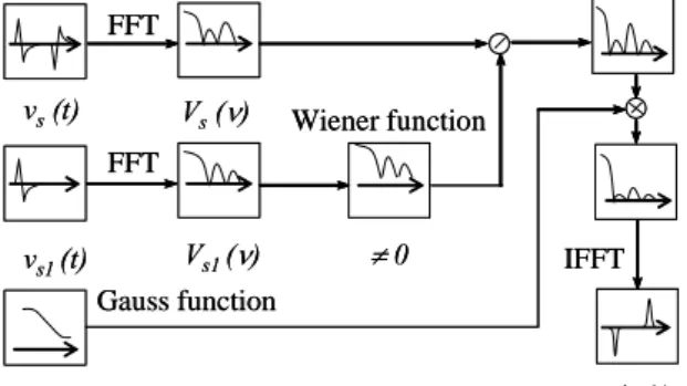
(see Equ. 12), and so for the test sample; iii/ errors due to the numerical processing of the signal, which is depicted in Fig. 4, and to the detection and acquisition system. vs(t) vs1 (t) Gauss function Vs1 (ν) Vs(ν) ≠0 FFT FFT IFFT Wiener function v’s(t) vs(t) vs1 (t) Gauss function Vs1 (ν) Vs(ν) ≠0 FFT FFT IFFT Wiener function v’s(t)

Figure 4: Synoptic of the signal processing implementation, according to Marc Jeroense.

Indeed, the signal passes by three principal filters, provided by the piezoelectric sensor, the amplifying circuit and the oscilloscope. It is thereafter digitized and processed numerically, through steps using Gauss and Wiener functions aimed at limiting the frequency range of the signal spectrum and avoiding division by zero in the Fourier space, respectively. The effect of Gaussian filter processing on space charge spreading is modeled in Fig. 5. Usually, noise is acceptably reduced with 1/g=2 as Matlab Gaussian filter parameter.

Electrical signal Time (µs) T h eor ical P iezo el ect ri c re spons e ( m V

) Space charge profile

Location (µm) S p ace char ge m odel e d dens it y (C /m 3) Matlab Gaussian parameter 1/g=2 Matlab Gaussian parameter 1/g=12 0.21µs Sound velocity: vp=2000m/s 420µm

Figure 5: Effect of a numerical processing by a Gaussian filter on space charge profile spreading.

Typically, for a situation of 2ns of sampling rate and 2000m/s of sound velocity, the spreading take up to 20µm. Using l/g=12, the peak width at mid-height would be around 96 µm.

CONCLUSION

This introduction to the PEA method we feel has show the origin of physical equations used to analyze PEA profiles. Important approximations are usually made in the analysis of PEA response, and these have been stressed in this presentation. Among these, we show the effect of signal processing by Gaussian filter on spreading of space charge profile.

Acknowledgement

Thanks are due to Dr. T. Maeno and K. Fukunaga from CRL, Tokyo, Japan, for providing technical assistance and helpful discussion.

REFERENCES

[1] J. Densley, R. N. Hampton, M. Henriksen, D. K. Das-Gupta, A. Toureille, R. Hegerberg, T. Takada, C. Alquie, J. T. Holboell, C. le-Gressus, S. Gubenald, G. Damanne, T. Tanaka, and M. Nagao, "Space charge measurements techniques: a review," Electra /

CIGRE, vol. 187, pp. 74-89, 1999.

[2] T. Takada, "Acoustic and optical methods for measuring electric charge distributions in dielectrics,"

IEEE Trans. Diel. & Elec. Insul., vol. 6, pp. 519-547,

1999.

[3] N. H. Ahmed and N. N. Srinivas, "Review of space charge measurements in dielectrics," IEEE Trans.

Diel. & Elec. Insul., vol. 4, pp. 644-56, 1997.

[4] T. Mizutani, " Space charge measurement techniques and space charge in polyethylene," IEEE

Trans. Diel. & Elec. Insul., vol. 1, pp. 923-33, 1994.

[5] P. Bloss and H. Schafer, "Investigations of polarization profiles in multilayer systems by using the laser intensity modulation method," Rev. Sci.

Instrum., vol. 65, pp. 1541-50, 1994.

[6] S. B. Lang and D. K. Das-Gupta, "Laser-intensity-modulation method: a technique for determination of spatial distributions of polarization and space charge in polymer electrets," J. of Appl. Phys., vol. 59, pp. 2151-60, 1986.

[7] P. Nothinger, S. Agnel, and A. Toureille, "Thermal step method for space charge measurements under applied dc field," IEEE Trans.Diele. & Elec. Insul., vol. 8, pp. 985-994, 2001.

[8] G. M. Sessler, "LIPP investigation of piezoelectricity distributions in PVDF poled with various methods," Ferroelectrics, vol. 76, pp. 489-96, 1987.

[9] Y. Satoh, Y. Tanaka, and T. Takada, "Improvement of piezoelectrically induced PWP method and its comparison with the PEA method,"

Elec. Eng. in Japan, vol. 121, pp. 1-7, 1997.

[10] T. Maeno, T. Futami, H. Kushibe, T. Takada, and C. M. Cooke, "Measurement of spatial charge distribution in thick dielectrics using the pulsed electroacoustic method," IEEE Trans. Diel. & Elec.

Insul., vol. 23, pp. 433-39, 1988.

[11] T. Maeno, "Calibration of pulsed electroacoustic method for measuring space charge density," T. IEE

Japan, vol. 119-A, pp. 1114-19, 1999.

[12] K. Fukunaga, "Industrial applications of space charge masurement in japan," in IEEE Elec. Insul.

Magazine, vol. 15 (5), 1999, pp. 6-18.

[13] P. Nothinger, A. Toureille, J. Santana, L. Martinotto, and M. Albertini, "Study of space charge accumulation in polyolefins submitted to ac stress,"

IEEE Transactions on Dielectrics and Electrical Insulation, vol. 8, pp. 972-984, 2001.

[14] A. S. De Reggi and S. Aimé, "Experimental methods for dielectric plarization measurements," presented at Interdisciplinary Conference on Dielectrics Short Course, 1992.

[15] P. Bloss, M. Steffen, H. Schafer, G. M. Yang, and G. M. Sessler, "A comparison of space-charge distributions in electron-beam irradiated FEP obtained by using heat-wave and pressure-pulse techniques," J.

Phys. D: Appl. Phys., vol. 30, pp. 1668-75, 1997.

[16] G. M. Sessler, C. Alquie, and J. Lewiner, "Charge distribution in Teflon FEP (fluoroethylenepropylene) negatively corona-charged to high potentials," J. of

Appl. Phys., vol. 71, pp. 2280-4, 1992..

[17] Y. Li and T. Takada, "Progress in space charge measurement of solid insulating materials in japan," in

IEEE Elec. Insul. Magazine, vol. 10 (5), 1994, pp.

16-28.

[18] N. Hozumi, Y. Muramoto, and M. Nagao, "Estimation of carrier mobility using space charge measurement technique," presented at CEIDP, Austin, T, USA, 1999.

[19] G. C. Montanari and I. Ghinello, "Space charge and electrical conduction-current measurements for the inference of electrical degradation threshold," Vide

Science, Tech. et Appli., vol. 287, pp. 302-11, 1998.

[20] J. M. Alison, "A high field pulsed electro-acoustic apparatus for space charge and external circuit current measurement within solid insulators,"

Meas. Sci. Technol., vol. 9, pp. 1737-1750, 1998.

[21] P. Morshuis and M. Jeroense, "Space charge measurements on impregnated paper: a review of the PEA method and a discussion of results," IEEE Elec.

Insul. Magazine, vol. 13, pp. 26-35, 1997.

[22] Y. Li, M. Aihara, K. Murata, Y. Tanaka, and T. Takada, "Space charge measurement in thick dielectric materials by pulsed electroacoustic method," Rev. Sci.

Instrum., vol. 66, pp. 3909, 1995.

[23] J. M. Alison, "The pulsed electro-acoustic method for the measurement of the dynamic space charge profile within insulators," in Space charge in

solid dielectrics, J. C. Fothergill and L. A. Dissado,

Eds. Leicester: The dielectrics Society, 1998, pp. 93-121.

[24] T. Maeno, "Calibration of pulsed electroacoustic method for measuring space charge density," T. IEE