A new shortest path algorithm to solve the resource-constrained project scheduling problem with routing from a flow solution

HAL Id: hal-01698361

https://hal.archives-ouvertes.fr/hal-01698361

Submitted on 4 Feb 2020

HAL is a multi-disciplinary open access

archive for the deposit and dissemination of

sci-entific research documents, whether they are

pub-lished or not. The documents may come from

teaching and research institutions in France or

abroad, or from public or private research centers.

L’archive ouverte pluridisciplinaire HAL, est

destinée au dépôt et à la diffusion de documents

scientifiques de niveau recherche, publiés ou non,

émanant des établissements d’enseignement et de

recherche français ou étrangers, des laboratoires

publics ou privés.

resource-constrained project scheduling problem with

routing from a flow solution

Philippe Lacomme, Aziz Moukrim, Alain Quilliot, Marina Vinot

To cite this version:

Philippe Lacomme, Aziz Moukrim, Alain Quilliot, Marina Vinot.

A new shortest path

al-gorithm to solve the resource-constrained project scheduling problem with routing from a

flow solution.

Engineering Applications of Artificial Intelligence, Elsevier, 2017, 66, pp.75-86.

�10.1016/j.engappai.2017.08.017�. �hal-01698361�

1

A New Shortest Path Algorithm to Solve the Resource-Constrained Project

Scheduling Problem with Routing from a Flow Solution

Philippe Lacomme

_{, Aziz Moukrim}

_{, Alain Quilliot}

_{Marina Vinot}

63177 Aubière Cedex, France.

b _{Sorbonne Universités, Université de Technologie de Compiègne, (Heudiasyc UMR CNRS 7253),}

CS 60 319, 60203 Compiègne France.

ARTICLE INFO ABSTRACT Article history: Received: Accepted: Available: Keywords: Routing Scheduling RCPSP Arc routing

In this study, the definition of a RCPSPR (Resource-Constrained Project Scheduling Problem with Routing) solution from a flow solution of the RCPSP is investigated. This new problem consists in defining a solution of RCPSPR that considers both routing and scheduling and that complies with a RCPSP flow, i.e., a solution where the loaded vehicle moves are achieved

between activity 𝑖 and 𝑗 with a non-null flow. A shortest path algorithm is proposed to solve

this problem with a labeling dynamic approach where a label provides all of the information about a solution, including the objective function, the system state and the remaining resources that allow the use of a dominance rule. The system state, described by the label, encompasses both the activities and the vehicle fleet information, including vehicle position and availability dates. Numerical experiments are limited to a comparative study with a proposed linear formulation since no previous publications exist on this problem. A time performance analysis of the proposed algorithm is carried out, proving the efficiency of the algorithm and clearing the way for integration into global iterative optimization schemes that will solve the RCPSPR to optimality.

1. Introduction

Although supply chain decision problems are interrelated, they are often solved sequentially. However, to achieve a highly effective overall system that complies with customers’ expectations, coordination among the different stages in the supply chain is necessary. Consequently, the integration of scheduling and routing problems has received increasing attention in the last decade (Moons et al., 2017). Several papers focusing on integrated problems were recently published, including but not limited to Zhang et al. (2016) who deal with the real-world production warehousing case, or Saglam and Banerjee (2017) who focus on batching decisions and different shipping scenarios. In supply chain management, in addition to the integration of production planning and distribution decisions, an effective management of the resources is essential to preserve the competitiveness of companies. This paper focuses on a new integrated problem based on the resource-constrained project scheduling problem with routing constraints.

1.1. Resource-constrained project scheduling problem

The Resource-Constrained Project Scheduling Problem (RCPSP) consists of a set of activities, 𝑉 = {0, . . . , 𝑛 + 1 }, with durations, 𝑝 = (𝑝0, . . . , 𝑝𝑛+1), where 𝑛 is the number of

non-dummy activities plus two non-dummy activities denoted 0 and 𝑛 + 1, which define the “project start” and the “project end”, respectively. The set of non-dummy activities is identified

1_{Corresponding author. e-mail addresses: placomme@isima.fr (P. Lacomme), aziz.moukrim@utc.fr (A. Moukrim), alain.quilliot@isima.fr (A.}

Quilliot), marina.vinot@isima.fr (M. Vinot)

by 𝐴 = {1, … , 𝑛} and some activities are related by precedence constraints. The precedence constraints can be induced by the definition of predecessors in the problem definition (one activity 𝑗 cannot start before all its predecessors have been achieved) and by definition of constraints due to the resource exchanges. A solution of the RCPSP is fully defined by the activity start times 𝑆𝑖 and by a resource supply that complies with the activity

requirements. The number of project resources is denoted as 𝑞

and the set of resource capacities is 𝑅 = {𝑅1, . . . , 𝑅𝑞},

where 𝑅𝑘∈ ℕ . The activity resource requirement 𝑏𝑖𝑘 ∈ ℕ

means that activity 𝑖 requires 𝑏𝑖𝑘 ≤ 𝐵𝑘 resource units of resource

𝑘 during its execution.

1.2. RCPSPR definition

The RCPSPR (Resource-Constrained Project Scheduling Problem with Routing) is an extension of the RCPSP where resources are transported from one activity to another using a vehicle. The problem consists of solving both the activity scheduling problem and the vehicle routing problem. This paper focuses on the case of one resource, 𝑞 = |𝑅| = 1, and assumes, without loss of generality, that 𝑏𝑖𝑘= 𝑏𝑖. The schedule length

𝐶𝑚𝑎𝑥 (i. e., the project makespan) is defined by the end of the last

transport operation from one activity to the dummy activity 𝑛 + 1.

The routing part consists of scheduling trips with a set of vehicles 𝑇 = {1, . . . , 𝑣 } sorted in descending order of capacity

2 𝑐𝑢, 𝑢 ∈ {1, … , 𝑣}. A loaded transportation time 𝑡𝑖𝑗𝑢𝑥 is defined

from activity 𝑖 to 𝑗 with a vehicle 𝑢 loaded with 𝑥 units of resources. An unloaded transportation time 𝑒𝑖𝑗𝑢 is also defined

from activity 𝑖 to 𝑗 with an empty vehicle 𝑢. An activity 𝑗 is defined by a starting time 𝑆𝑗 with a completion time 𝐶𝑗= 𝑆𝑗+

𝑝𝑗 and resource supplies that meet the requirement 𝑏𝑗. An

activity can only start when a total amount 𝑏𝑗 of resources is

transferred from activity i to activity 𝑗.

The resources transferred from activity 𝑖 to 𝑗 are modeled by a

transport operation 𝑇(𝑖,𝑗,𝑢,𝑥) = (𝑃(𝑖,𝑗,𝑢,𝑥) , 𝐷(𝑖,𝑗,𝑢,𝑥) ), which is

fully defined by a pickup operation 𝑃_{(𝑖,𝑗,𝑢,𝑥)} and a delivery operation 𝐷(𝑖,𝑗,𝑢,𝑦) . These two operations are defined by:

 an arrival time and a departure time of the vehicle, 𝐴 (𝑖,𝑗,𝑢,𝑥) and 𝐵(𝑖,𝑗,𝑢,𝑥), respectively;

 a quantity of resource (pickup or deliver) 𝑥;

 a vehicle assigned to the transport operation 𝑢.

The problem consists in a proper coordination of scheduling and

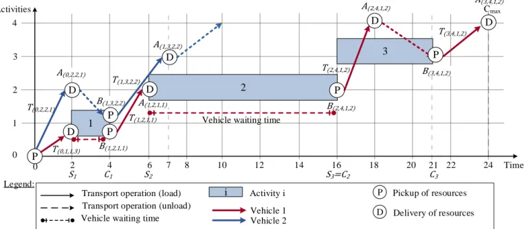
routing operations to minimize the makespan 𝐶𝑚𝑎𝑥 (Fig. 1). A

routing solution is defined as a set of trips, and each trip is an ordered sequence of loaded transport operations. The earliest starting time of an activity is the latest arrival time of the last vehicle assigned to the transportation of resources required by the activity.

In Fig. 1, an extended Gantt diagramdisplays a solution with the

earliest starting times and the durations of three activities, plus the trips of two vehicles with 𝑐₁= 3 and 𝑐₂= 2. For example, in Fig. 1, activity 1 has an earliest starting time equal to the arrival time 𝐴_(0,1,1,3) = 2. For activity 3, the earliest starting time is equal to the maximum value between the arrival time of vehicle 2 with two units of resource, 𝐴_(1,3,2,2)= 7 and the earliest completion time of activity 2, 𝐶₂= 16, due to a precedence constraint. Let us note that the earliest starting time of activity 2, is the latest arrival time of the vehicles (vehicle 1), meaning that two delivery operation are required to define the starting time of activity 2.

2 3

4

Transport operation (load) Transport operation (unload)

Time 2

0 0

Vehicle waiting time 4 1 A(1,2,1,1) 2 3 i Activity i D P Delivery of resources Pickup of resources Cmax 8 6 7 10 12 14 16 18 20 22 24 Legend: 1 S1 C1 S2 S3=C2 C3 21 Activities P D T(0,1,1,3) P D T(1,2,1,1) P D B(2,4,1,2) A(2,4,1,2) T(2,4,1,2) _B(3,4,1,2) P A(3,4,1,2) D T(3,4,1,2)

Vehicle waiting time T(0,2,2,1) A(0,2,2,1) D B(1,3,2,2) P B(1,2,1,1) A(1,3,2,2) D T(1,3,2,2) Vehicle 1 Vehicle 2

Figure 1. Coordination between routing and scheduling

In this example, vehicle 2 transports one resource from activity 0 to 2 (𝑇(0,2,2,1)) and then makes an unloaded move to activity 1

in order to load and transport two resources to activity 3 (𝑇(1,3,2,2)). Once the resources are delivered at time 7, vehicle 2

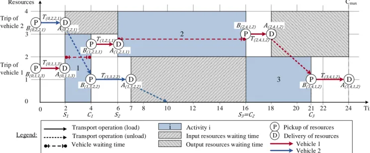
goes back to the depot and arrives at time 10. Figure 2 shows that two deliveries are performed on activity 2, the first delivery operation permits to transport one unit of resource from activity 0 with the vehicle 2 and the second delivery operation permits to transport one unit from activity 1 thanks to vehicle 1. The

delivery operation are defined by both a location (activity) and a quantity of resource. The resource delivered at one activity are assumed to be in an input buffer on the activity. Such situation occurs for activity 2, where one unit of resource waits from time 2 to time 6 in the input buffer of activity 2. At time 6, activity 2 can start thanks to the transport operation 𝑇(1,2,1,1). This example

is used throughout the paper in order to illustrate the proposed algorithm.

3

2 3

4

Transport operation (load) Transport operation (unload) Resources

Time 2

0 0

Output resources waiting time Vehicle waiting time

4 1 2 A(1,2,1,1) 3 A(0,1,1,3) B(0,1,1,3) P D A(0,2,2,1) D P B(1,3,2,2) P B(1,2,1,1)

Input resources waiting time

i Activity i D P Delivery of resources Pickup of resources Cmax 8 6 10 12 14 16 18 20 22 24 P B(3,4,1,2) P A(3,4,1,2) D 7 D A(1,3,2,2) D D Legend: Trip of vehicle 1 B(0,2,2,1) P Trip of vehicle 2 B(2,4,1,2) A(2,4,1,2) T(0,2,2,1) T(0,1,1,3) T(1,3,2,2) T(1,2,1,1) T(2,4,1,2) T(3,4,1,2) 1 S1 C1 S2 S3=C2 C3 21 Vehicle 1 Vehicle 2

Figure 2. Impact of coordination on the ressource management

1.3. Related problems

Routing constraints are involved in numerous scheduling problems including, for example, the flexible job-shop scheduling problem with transport (Zhang et al., 2012b), the job-shop with transport (Knust, 1999; Lacomme et al., 2013; Afsar et al., 2016), the Flexible Manufacturing Systems (FMS) (Caumond et al., 2009), the HSP (Hoist Scheduling Problem) (Honglin et al., 2016; Adnen and Mohsen, 2016; Chtourou et al., 2013), and the RCPSP with transport (Quilliot et al., 2012). Numerous scheduling approaches take advantage of the disjunctive graph introduced by Roy et al. (1964), which has been extended to tackle transport constraints (see Lacomme et al. (2007) and Zhang et al. (2012a)), where vertex models transport operations and disjunctive arcs are added between operations that require the same resource (vehicle). The coordination between transport and scheduling can be achieved in two possible ways depending on the objective. The first one consists of the explicit modeling of transport from one location to another, and the second one consists in modeling only transport delay (minimal time-lags between machines). Maximal time-lags between activities can model a time window between activities and are used in pickup and delivery resolution approaches for trip evaluation (Cordeau and Laporte, 2003; Firat and Woeginger, 2011).

Transport modeling depends on the vehicle capacity, and a trip is considered to be an ordered sequence of pickup/delivery operations including loaded/unloaded transport operations. Depending on the problem, the transportation time can be job/vehicle load-dependent and can be denoted 𝑡𝑖𝑗𝑥 for a transport

from activity 𝑖 to 𝑗 with 𝑥 resources. Similarly, 𝑡_𝑖𝑗0 (normally denoted 𝑒𝑖𝑗 = 𝑡𝑖𝑗0) denotes the duration of an unloaded transport

operation. If the transportation times are vehicle-dependent, they can be noted 𝑡𝑖𝑗𝑢𝑥 where 𝑢 is the vehicle.

2. Proposition

2.1. RCPSPR modeling

Several formulations were introduced for the RCPSP, including

Alvarez-Valdés and Tamarit (1993), Pritsker et al. (1969), Pritsker and Watters (1968) and Dauzère-Pérès and Lasserre, (1995), and more recently, the flow formulation of Artigues et al. (2003) that defines a solution of the RCPSP using an

activity-on-node (AON)-flow network defining a so called 𝐺_𝐴𝑂𝑁𝜑 ( 𝑉, 𝐸)

(Fig. 3). In this graph, there is a vertex in 𝑉 for each activity. In addition, the set 𝐸 of resource arcs represents the number of units of the resource directly transferred between two activities. The arc in Fig. 3 between node 0 and 𝑖1 models a resource

transfer of 𝜑0,𝑖1 units of the resource between activity 0 and 𝑖1.

ϕ

0

i

i

i

i

i

i

i

...

ϕ

ϕ

ϕ

ϕ

ϕ

ϕ

i

p

0

i1

i2

ip

...

0

0

0

p

p

_p

i.

Figure 4. Disjunctive graph 𝐷𝐺_𝐴𝑂𝑁𝜑 ( 𝑉, 𝐸)

A disjunctive graph 𝐷𝐺_𝐴𝑂𝑁𝜑 ( 𝑉, 𝐸) (Fig. 4) is defined considering

the (AON)-flow network 𝐺𝐴𝑂𝑁𝜑 ( 𝑉, 𝐸) graph. For each node, 𝑖 ∈

𝑉, all outgoing arcs (𝑖, 𝑗) ∈ 𝐸 are weighted by the duration 𝑝𝑖 of

4 since activity 𝑗 has to be scheduled after activity 𝑖. The longest

path from 0 to 𝑛 + 1 in graph 𝐷𝐺𝐴𝑂𝑁𝜑 ( 𝑉, 𝐸) makes it possible to

obtain the earliest starting time of all activities and a critical path. The dashed arc in Fig. 4 models a precedence constraint between the activities.

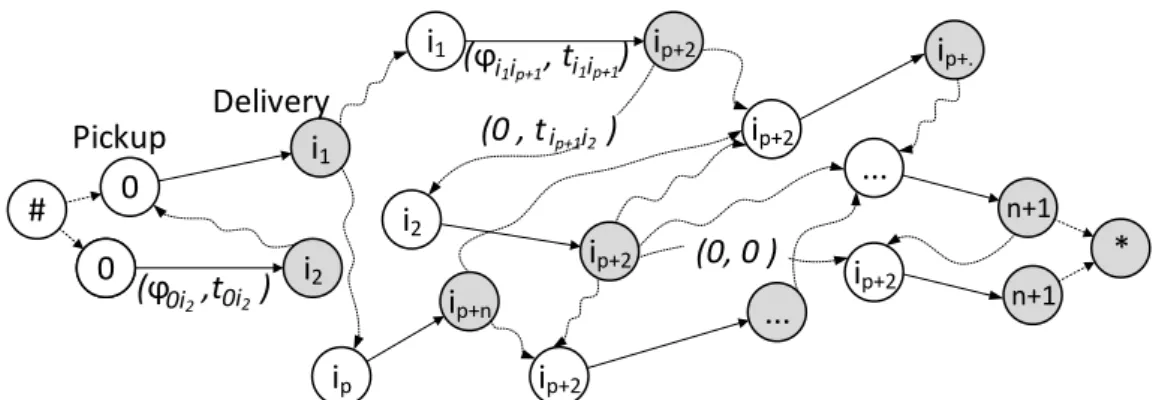
𝐺_𝐴𝑂𝑁𝜑 ( 𝑉, 𝐸) and 𝐷𝐺_𝐴𝑂𝑁𝜑 ( 𝑉, 𝐸) make it possible to define a graph 𝑇𝜑_{( 𝑈, 𝑉, 𝐸, 𝐹), which explicitly models the activities and the}

transport operations of the RCPSPR. In our problem, the arc routing transportation graph 𝑇𝜑( 𝑈, 𝑉, 𝐸, 𝐹) uses two types of arcs (Lacomme et al., 2005):

 required arc (𝑖, 𝑗) ∈ 𝐸 corresponding to a positive flow transfer and consequently defining loaded transport operations. A required arc can be serviced by several trips depending on the total demand and on vehicle capacities.

 non-required arcs (𝑖, 𝑗) ∈ 𝐹 corresponding to a null flow and

that can be used for an unloaded transport operation. Non-required arcs make it possible to define deadheading paths

from 𝑖 to 𝑗.

In the graph 𝑇𝜑( 𝑈, 𝑉, 𝐸, 𝐹), the vertices are divided into two disjointed sets:

 𝑈: the pickup node set (in white in Fig 5);

 𝑉: the delivery node set (in gray in Fig 5).

Every arc 𝑒 ∈ 𝐸 connects a vertex in 𝑈 to a vertex in 𝑉 to model a loaded transport operation, |𝐸| = 𝑛𝜑, and every arc 𝑓 ∈

𝐹 connects a vertex from 𝑉 to a vertex 𝑈 to model an unloaded transport operation (dotted arcs in Fig. 5).

The required arcs (arcs modeling loaded transport operations) are defined by a couple (𝜑𝑖𝑗, 𝑡𝑖𝑗) where 𝜑𝑖𝑗 is the number of

resources to transport from 𝑖 to 𝑗 and where 𝑡𝑖𝑗 is the

transportation time. The valuation of a non-required arc (an arc modeling an unloaded transport operation) is defined by (0, 𝑡𝑗𝑣).

For convenience, two global dummy nodes are introduced, the first one referred to as # to represent the starting time of the first transport operation, and the second one ∗, the finishing time of the last transport operation.

0

i

i

i

i

i

i

i

Pickup

Delivery

i

...

...

0

i

(ϕ , t

)

(0 , t

)

i

i

i

(ϕ ,t

)

(0, 0 )

0

#

*

Figure 5. Arc Routing Transportation Graph 𝑇𝜑(𝑈, 𝑉, 𝐸, 𝐹)

A solution of the RCPSPR is composed of a set of trips assigned to vehicles, knowing that a trip is composed of an ordered set of required arcs and a deadheading path from the destination node of one required arc to the origin node of the next required arc in the trip:

 First, from this point of view, the problem to solve falls into the family of arc routing problems, including, for example, the Chinese Postman Problem (CPP) first introduced by the mathematician Kwan (1962), the Rural Postman Problem (RPP) (Orloff, 1974), and the Capacitated Arc Routing Problem (CARP), that was introduced by Golden and Wong (1981). Contrary to the CARP, where the vehicle load increases during the trip, the pickup/delivery characteristics lead to a specific arc routing problem with no trip infeasibility due to vehicle capacity.

 Second, the problem can be solved using a resolution

approach based on a labeling algorithm with an efficient label processing procedure and a specific label definition that makes it possible to obtain a solution of a resource-constrained shortest path problem.

An optimal solution of the RCPSPR defined by the flow can be obtained by execution into 𝑇𝜑( 𝑈, 𝑉, 𝐸, 𝐹) of a shortest path algorithm with resource constraints between the global dummy nodes # and ∗. The shortest path is defined by an ordered sequence of transport operations with alternation between loaded transport and unloaded transport operations.

2.2. RCPSPR solution defined from a flow

A flow solution defines an acyclic graph 𝐺𝐴𝑂𝑁𝜑 ( 𝑉, 𝐸) where the

flow arcs can make it possible to define the transport operations with the quantity of resource. The flow is assumed to comply with the definition of Artigues et al. (2003), and the input/output flow of an activity is assumed to be equal to its required capacity with flow conservation. A flow 𝜑𝑖𝑗 between activity 𝑖 and

activity 𝑗 can exceed the vehicle capacity and can require several transport operations due to the vehicle capacity constraints (𝑐𝑣).

The new algorithm dedicated to the resource-constrained shortest path problem is defined on a non-ordered set of transport operations and provides an optimal set of trips to build both a routing solution and a scheduling solution that consists of:

 computing the earliest starting times 𝑆𝑖 of the activities;

 defining the assignment of vehicles to transport operations;

 ordering the transport operations for each vehicle to define a trip with the departure time and arrival time of the vehicle for each transport operation.

The transport operations are divided into two categories with:

 Loaded transport operation 𝑇𝑖,𝑗,∗,𝜑_𝑖𝑗 from activity 𝑖 to 𝑗,

5 composed of the flow 𝜑𝑖𝑗 (that must be transported from

activity 𝑖 and activity 𝑗) and the transportation time 𝑡𝑖𝑗.

 Unloaded transport operation, modeled by an arc (dotted arcs

in Fig. 5) valuated with 0 for the flow and 𝑡𝑖𝑗 for the

transportation time.

2.3. A New Shortest Path Algorithm and its application to arc routing

The resource-constrained shortest path problem considered in this paper makes it possible to define an optimal solution of the

RCPSPR in the graph 𝑇𝜑_{(𝑈, 𝑉, 𝐸, 𝐹). Each solution (Fig. 6) is}

composed of a set of trips (modeled by a path in 𝑇𝜑_{(𝑈, 𝑉, 𝐸, 𝐹)}

from node # to node ∗) passing through every arc with a non-null flow. The solution is optimal if it minimizes the arrival time of all the vehicles on the node ∗ with respect to all the constraints. Figure 6 shows two trips assigned to two vehicles. The trip of vehicle 1 is composed of six transport operations, whereas the trip of vehicle 2 consists of three transport operations. These two trips are interrelated due to some activities in both trips, e.g. activity 𝑖𝑝+2. The two delivery nodes 𝑖𝑝+2 must

be scheduled before the two pickup nodes 𝑖𝑝+2, and the

departure times of the two loaded transport operations from the two pickup nodes 𝑖_𝑝+2 are greater or equal to the completion time of the activity 𝑖𝑝+2.

0

i1

i1

ip+.

i2

...

...

0

i2

ip

#

*

Legend : _{Loaded transport operation}

Unloaded transport operation

Vehicle 1 Vehicle 2

Figure 6. A solution with two trips in the graph 𝑇𝜑(𝑈, 𝑉, 𝐸, 𝐹)

Each partial solution (also denoted for convenience as a solution) is modeled by a path represented by a label 𝐿(𝑓, 𝑆, 𝑅) i.e., a data structure that provides all of the information about the solution such as the objective function, the system state and the remaining resources that allow the use of a dominance rule. A partial solution is defined by a label where all the flows between operations have not yet been transported by vehicles, meaning that all activities are not yet scheduled. Conversely, a final solution is a label where all flows have been transported, i.e., a label where all activities have been scheduled.

For each node 𝑖 of the graph 𝑇𝜑_{(𝑈, 𝑉, 𝐸, 𝐹), 𝑌}

𝑖 is the ordered set

of unprocessed labels, i.e., paths that have not been extended along all arcs (𝑖, 𝑗) leading to feasible paths. The set 𝑃𝑖 contains

labels that are required to be kept, i.e., 𝑃𝑖 defines a set of

non-dominated labels on node 𝑖. The labels are sorted into non-decreasing order of the total loaded transportation time 𝑡𝑖𝑗 from

activity 𝑖 to 𝑗 not yet serviced according to the required flow, and 𝑍𝑖 is the restriction of 𝑌𝑖 to the 𝑁𝐿first labels.

For each node 𝑖, the distance 𝐷[𝑖] is the longest path in terms of the number of arcs from 𝑖 to the dummy node * . In other words, 𝐷[𝑖] is a distance between a partial solution and a solution of the

problem and is representative of the computational effort required to obtain a final solution. The distances are preprocessed and are directly used in the following algorithm. The use of a dominance rule is optional in the sense that the algorithm otherwise enumerates all feasible paths starting at node #, but dominance is crucial in the design of one efficient resource-constrained shortest path algorithm to identify paths that do not need to be extended.

The outline of the resource-constrained shortest path algorithm for solving the RCPSPR is presented in Algorithm 1. The problem consists of computing a minimum-cost feasible path ending at the global dummy nodes * where a set of non-dominated labels (each label modeling a partial solution) is stored. The algorithm starts with one initialization step (lines 12-15) where a label 𝐿0 is stored on the global dummy node # (that

models the depot node of vehicles). Lines 16-34 define the outer loop where labels are propagated along feasible-path constraints. The algorithm terminates when no further unprocessed label on the node exists, i.e., when all labels giving the non-dominated paths from vertex # to * have been created, which is defined by an empty queue Λ. The algorithm selects a final solution 𝑆𝑜𝑙 (line 35) that minimizes the objective function 𝑓.

6

Procedure name: New Shortest Path Algorithm

1. procedure Shortest_Path 2. input parameters

2. 𝑇𝜑_{( 𝑈, 𝑉, 𝐸, 𝐹): Arc routing transportation graph}

3. 𝑈𝐵: Upper Bound of the problem

4. 𝐿𝐵𝑖: Lower Bound to reach the final node from node 𝑖

5. output parameters 6. 𝑆𝑜𝑙: Solution 7. global parameter 8. Λ: Queue

9. 𝑛_𝑣𝑒ℎ𝑖𝑐𝑙𝑒: number of vehicles

10. 𝑁𝐿: maximum number of unprocessed labels into 𝑍𝑖 ∈ 𝑈∪𝑉

11. begin

12. Definition of 𝐿𝑜

13. for 𝑛𝑜𝑑𝑒_𝑖 ∈ 𝑈 ∪ 𝑉 do

14. if (𝜆(𝑛𝑜𝑑𝑒_𝑖) = 0) then 𝑍node_i= {𝐿𝑜},𝑃𝑈𝑆𝐻(Λ, 𝑛𝑜𝑑𝑒_𝑖) else 𝑃node_i= {∅} endif

15. endfor

16. while (Λ ! = ∅) do 17. 𝑛𝑜𝑑𝑒_𝑖 ∶= 𝑃𝑂𝑃(Λ)

18. for 𝐿𝑖∈ 𝑍node_i do //for each label unprocessed on node i

19. for 𝑛𝑜𝑑𝑒_𝑗 ∈ 𝑠𝑢𝑐𝑐(𝑛𝑜𝑑𝑒_𝑖)do

20. if 𝑃𝐴𝑇𝐻(𝐿𝑖, 𝑛𝑜𝑑𝑒_𝑗) 𝑖𝑠 𝑓𝑒𝑎𝑠𝑖𝑏𝑙𝑒 then //resources and precedence constraints

21. for 𝑣: = 1 to 𝑛_𝑣𝑒ℎ𝑖𝑐𝑙𝑒 do 22. call 𝐶𝑅𝐸𝐴𝑇𝐸_𝐿𝐴𝐵𝐸𝐿(𝐿𝑤, 𝑣, 𝐿𝑖, 𝑛𝑜𝑑𝑒𝑖, 𝑛𝑜𝑑𝑒𝑗) 23. if (𝐷𝑂𝑀𝐼𝑁𝐴𝑇𝐸(𝐿𝑤, 𝑛𝑜𝑑𝑒_𝑗)) and (𝐶𝐻𝐸𝐶𝐾_𝑈𝐵_𝐿𝐵(𝐿𝑤, 𝐿𝐵𝑛𝑜𝑑𝑒_𝑗, 𝑈𝐵)) then 24. call 𝐼𝑁𝑆𝐸𝑅𝑇_𝐿𝐴𝐵𝐸𝐿(𝐿𝑤, 𝑍𝑛𝑜𝑑𝑒_𝑗), call 𝑃𝑈𝑆𝐻(Λ, 𝑛𝑜𝑑𝑒_𝑗), 25. call 𝐴𝑃𝑃𝐿𝑌_𝐷𝑂𝑀𝐼𝑁𝐴𝑁𝐶𝐸(𝐿𝑤, 𝑍𝑛𝑜𝑑𝑒_𝑗) 26. endif

27. if (𝜆(𝑛𝑜𝑑𝑒_𝑗) = ∗) then call 𝐶𝐻𝐸𝐶𝐾_𝑆𝑂𝐿(𝐿_𝑤, 𝑈𝐵) endif 28. endfor 29. endfif 30. endfor 31. 𝑍node_i = 𝑍node_i \ 𝐿𝑖 32. 𝑃node_i = 𝑃node_i ∪ 𝐿𝑖 33. endfor 34. endwhile

35. 𝑆𝑜𝑙 ∶= 𝐵𝐸𝑆𝑇_𝑆𝑂𝐿 (𝑇𝜑_{) //save the best solution}

36. end

Algorithm 1. New shortest path procedure.

The Boolean function 𝐷𝑂𝑀𝐼𝑁𝐴𝑇𝐸(𝑖, 𝑗) (line 23) return true if the label 𝑖 is not dominated by an unprocessed label on node 𝑗.

𝐷𝑂𝑀𝐼𝑁𝐴𝑇𝐸(𝑖, 𝑗) = ∄𝑘 ∈ 𝑍𝑗, 𝑘 ≪ 𝑖 (1)

The algorithm also uses the function 𝐶𝐻𝐸𝐶𝐾_𝑈𝐵_𝐿𝐵(𝐿, 𝐿𝐵, 𝑈𝐵)

(line 23), which returns true if the label 𝐿 cannot be pruned, and false if the objective function of the label 𝐿 plus the lower bound 𝐿𝐵 does not fit the upper bound 𝑈𝐵.

The label feasibility is checked considering the remaining resources in the function 𝑃𝐴𝑇𝐻(𝐿𝑖, 𝑛𝑜𝑑𝑒_𝑗). The propagation rule

to create a new label (detailed below) is achieved by the procedure 𝐶𝑅𝐸𝐴𝑇𝐸_𝐿𝐴𝐵𝐸𝐿(𝐿𝑤, 𝑣, 𝐿_𝑖, 𝑛𝑜𝑑𝑒𝑖, 𝑛𝑜𝑑𝑒𝑗) (line 22),

which makes it possible to obtain a new label 𝐿𝑤 from label 𝐿𝑖

considering vehicle 𝑣. The procedure

𝐼𝑁𝑆𝐸𝑅𝑇_𝐿𝐴𝐵𝐸𝐿(𝐿𝑤, 𝑍𝑛𝑜𝑑𝑒_𝑗) (line 24) carries out the insertion of

the label 𝐿𝑤 in the ordered set of unprocessed labels 𝑍𝑛𝑜𝑑𝑒_𝑗 that

take the maximum number of unprocessed labels authorized on

each node 𝑁_𝐿 into account. Then, with the function

𝐴𝑃𝑃𝐿𝑌_𝐷𝑂𝑀𝐼𝑁𝐴𝑁𝐶𝐸(𝐿𝑤, 𝑍𝑛𝑜𝑑𝑒_𝑗) (line 25), all labels on 𝑍𝑛𝑜𝑑𝑒_𝑗

that are dominated by 𝐿𝑤 are removed from 𝑍𝑛𝑜𝑑𝑒_𝑗.

The 𝐶𝐻𝐸𝐶𝐾_𝑆𝑂𝐿(𝐿𝑤, 𝑈𝐵) (line 27) function updates the upper

bound of the problem for each new solution (defining a path through every arc with a non-null flow) on the final node. Finally,

the best solution at the end of the algorithm is given by the function 𝐵𝐸𝑆𝑇_𝑆𝑂𝐿 (𝑇𝜑) (line 35) from the best final label in 𝑇𝜑. The resource-constrained shortest path algorithm must encompass the management of both the availability of vehicles and that of activities, and includes the following features:

 a label definition to encompass the system state;

 creation of the initial label;

 a propagation rule to create a new label;

 a label feasibility check;

 a dominance rule to save only non-dominated labels on the node.

 a label propagation selection rule required to choose the next path (next label) to be extended.

Let us define a function that makes it possible to assign a number in [1. . 𝑛𝜑] to each arc.

β: 𝑒 ∈ 𝐸 → [1. . 𝑛𝜑] ,

β(𝑒 ∈ 𝐸 ) = 𝑖

∀𝑒1∈ 𝐸, ∀𝑒2∈ 𝐸, 𝑒1≠ 𝑒2, β(𝑒1) ≠ β(𝑒2 ).

Another notation is also used to identify the pickup node and the delivery node of each numbered arc 𝑖 𝜖 [1. . 𝑛𝜑]. Let us denote 𝑖+

as the position number of the pickup node in graph 𝐺 and 𝑖− _as

7 activity number where a pickup operation (resp. delivery

operation) is achieved from position 𝑖+ _{(resp. 𝑖}−_{) such that 𝜆(𝑖}−₎

or 𝜆(𝑖+_{) gives the activity where the operations are achieved.}

Label definition

A label 𝐿 = (𝑓, 𝑆, 𝑅) represents a partial or final solution and 𝐿𝑗𝑖

denotes the 𝑖𝑡ℎ _{label on node 𝑗 = 𝑗}− _{or 𝑗 = 𝑗}+_{, which is composed}

of three parts:

 The objective function value of the solution, i. e., the maximal completion time of the vehicles.

 The system state 𝑆 that encompasses the vehicle fleet and the

activities. The system state can be described by:

- a 3𝑣-uplet 𝑉_𝑖𝑗 defining the vehicle departure and arrival

times, and positions, 𝑉_𝑖𝑗=

( 𝑃𝑖𝑗1, … , 𝑃𝑖𝑗𝑣, 𝐴1𝑖𝑗, … , 𝐴𝑖𝑗𝑣, 𝐵𝑖𝑗1, … , 𝐵𝑖𝑗𝑣), where 𝑃𝑖𝑗1, … , 𝑃𝑖𝑗 𝑣

are the current position of each vehicle (𝑃𝑖𝑗𝑢= 𝑝 means

that the position of the vehicle 𝑢 is on activity 𝑝), 𝐴1𝑖𝑗, … , 𝐴𝑖𝑗𝑣 are the arrival times, and 𝐵𝑖𝑗1, … , 𝐵𝑖𝑗𝑣 are the

departure times of the vehicles;

- a 𝑛 + 1-uplet 𝑆_𝑖𝑗 defining the earliest starting time of each activity 𝑆_𝑖𝑗 = ( 𝑆𝑖𝑗 0, … , 𝑆𝑖𝑗𝑛+1).

 The resource state 𝑅 remaining on arcs modeling loaded transport operations (required arcs) and the remaining number of resources to start each activity:

- a 𝑛_𝜑-uplet 𝜑_𝑖𝑅,𝑗 = ( 𝜑_𝑖𝑗 𝑅,1, … , 𝜑_𝑖𝑗𝑅,𝑛𝜑) defining the remaining resources of the arc 𝑒 ∈ 𝐸; 𝜑_𝑖𝑗 𝑅,β(𝑒) not yet transported;

- a 𝑛 + 1-uplet 𝑏_𝑖𝑅,𝑗 = ( 𝑏_𝑖𝑗 𝑅,0, … , 𝑏_𝑖𝑗𝑅,𝑛+1) defining the remaining resources 𝑏_𝑖𝑗 𝑅,𝑘 for activity 𝑘 not yet transported.

Creation of the initial label

An initial label 𝐿 is stored on node # and propagated to all nodes

𝑗 = 𝑗+_{, where 𝜆(𝑗}+_{) = 0. To comply with the following}

definition, all the values are initialized: ∀𝑢 ∈ 𝑇, 𝑃1𝑗𝑢 = 0 ∀𝑢 ∈ 𝑇, 𝐴1𝑗𝑢 = 0 ∀𝑢 ∈ 𝑇, 𝐵1𝑗𝑢 = 0 ∀𝑘 ∈ 𝑉∗_{, 𝑆} 1𝑗𝑘 = −∞ and 𝑆1𝑗0 = 0 ∀𝑖 ∈ [1. . 𝑛𝜑], 𝜑1𝑗𝑅,𝑖 = 𝜑λ(𝑗+_),λ(𝑗−₎ ∀𝑘 ∈ 𝑉, 𝑏𝑞𝑗 𝑅,𝑘= 𝑏k 𝑓1𝑗= 0

Propagation rule for a label on a pickup node (arc modeling a loaded transport operation)

A propagation function defined by 𝑓: L  T → R that makes the

propagation of a new label 𝐿𝑖_𝑞− from one label 𝐿_𝑝𝑖+ and a loaded transport operation defined by (𝜑𝑚𝑘, 𝑡𝑚𝑘) /𝑚 = 𝜆(𝑖+) and 𝑘 =

𝜆(𝑖−_{) possible.}

The new label 𝐿_𝑞𝑗 for node number 𝑗 = 𝑖− is defined from the label 𝐿𝑖𝑝 𝑖 = 𝑖+ using the vehicle 𝑢 with the following updates:

𝑃𝑞𝑗𝑢 = 𝜆(𝑗) 𝐴𝑞𝑗𝑢 = 𝐵𝑝𝑖𝑢 + 𝑡𝜆(𝑖),𝜆(𝑗) 𝐵𝑞𝑗𝑢 = 𝐴𝑞𝑗𝑢 𝑆_𝑞𝑗𝜆(𝑗)= 𝑚𝑎𝑥 (𝐴𝑞𝑗𝑢; 𝑆𝑝𝑖𝜆(𝑗)) 𝜑_𝑞𝑗𝑅,𝑖 _{= 𝜑} 𝑝𝑖𝑅,𝑖 − 𝑚 𝑖𝑛( 𝜑𝑝𝑖 𝑅,𝑖; 𝑐𝑢) 𝑏_𝑞𝑗 𝑅,𝜆(𝑗)= 𝑏_𝑝𝑖 𝑅,𝜆(𝑗)− 𝑚 𝑖𝑛( 𝜑𝑝𝑖 𝑅,𝑖; 𝑐𝑢) 𝑓𝑞𝑗= 𝑚𝑎𝑥 (𝑓𝑝𝑖; 𝐴𝑢𝑞𝑗)

If 𝑏_𝑞𝑗 𝑅,𝜆(𝑗)= 0, the propagation rule also updates all the starting

times of the successors of activity 𝜆(𝑖), i.e., ∀𝑠 ∈

𝑠𝑢𝑐𝑐(𝜆(𝑖)), 𝑆𝑞𝑗𝑠 = 𝑚𝑎𝑥(𝑆𝑝𝑖𝑠; 𝑆𝑞𝑗𝜆(𝑗)+ 𝑝𝜆(𝑗)). This update ensures

that precedence constraints hold. For the label 𝐿𝑖𝑝, all assignments

to vehicles are investigated, leading to 𝑣 labels. These labels are included or not depending on the set of non-dominated labels previously stored on the node 𝑗 in 𝑇𝜑_{( 𝑈, 𝑉, 𝐸, 𝐹).}

Propagation rule for a label on a delivery node (arc modeling an unloaded transport operation)

A propagation function defined by 𝑓: L  T → R that makes the

generation of a new label 𝐿𝑗𝑞

−

from one label 𝐿𝑖𝑝+ and an unloaded

transport operation defined by (0, 𝑡𝑚𝑘)/𝑚 = 𝜆(𝑗−) and 𝑘 =

𝜆(𝑖+_{) possible.}

The new label 𝐿𝑗𝑞 with 𝑗 = 𝑖+ is defined from the label 𝐿𝑖𝑝, where

𝑖 = 𝑗− _{using vehicle 𝑢 with the following updates:}

𝑃𝑞𝑗𝑢 = 𝜆(𝑗) 𝐴𝑞𝑗𝑢 = 𝐵𝑝𝑖𝑢 + 𝑒𝜆(𝑖),𝜆(𝑗) 𝐵𝑞𝑗𝑢 = 𝑚𝑎𝑥 (𝐴𝑞𝑗𝑢; 𝑆𝑝𝑖 𝜆(𝑗) + 𝑝𝜆(𝑗)) 𝑓𝑞𝑗= 𝑚𝑎𝑥 (𝑓𝑝𝑖; 𝐴𝑢𝑞𝑗)

Label feasibility check

The first and the second conditions detailed below only hold for label 𝐿𝑖𝑞− stored at delivery node 𝑖 = 𝑖− propagated to a pickup

node 𝑗 = 𝑗+_{. Both conditions are linked to the resource state. The} first condition takes advantage of the flow. If the flow 𝜑_𝑞𝑖𝑅,𝑗 = 0,

i.e., all resources between 𝜆(𝑗+_{) and 𝜆(𝑗}−_{) were transported, then}

an unloaded transport operation to activity 𝜆(𝑗+) must be forbidden. The second condition holds since an unloaded transport operation can only be achieved to an activity 𝜆(𝑗+) previously scheduled, i.e., for which all the resources were delivered 𝑏_𝑞𝑖 𝑅,𝜆(𝑗)= 0. If 𝑏_𝑞𝑖 𝑅,𝜆(𝑗)≠ 0, no unloaded transportation operation to 𝜆(𝑗+_{) must be scheduled.}

Dominance rule

Whenever one or several new labels are created (by the propagation rule), they are compared for dominance with the non-dominated labels that are stored at the destination node. Considering two labels 𝐿𝑖𝑝 and 𝐿𝑖𝑞, 𝐿𝑖𝑝 is defined as dominant as

regards 𝐿𝑖𝑞 ( 𝐿𝑞𝑖 ≪ 𝐿𝑖𝑝) if the following conditions hold:

Condition 1. All vehicles have the same location:

8 Condition 2. ∀𝑢 ∈ 𝑇, 𝐵_𝑖𝑝𝑢 ≤ 𝐵_𝑖𝑞𝑢 Condition 3. ∀𝑢 ∈ 𝑇, 𝐴_𝑖𝑝𝑢 ≤ 𝐴_𝑖𝑞𝑢 Condition 4. ∀𝑘 𝜖 [1. . 𝑛𝜑], 𝜑𝑖𝑝𝑅,𝑘 ≤ 𝜑𝑖𝑞𝑅,𝑘 Condition 5. 𝑆_𝑖𝑝𝑛+1≤ 𝑆_𝑖𝑝𝑛+1 Condition 6. ∃𝑢 ∈ 𝑇, 𝐵𝑖𝑝𝑢 < 𝐵𝑖𝑞𝑢 or ∃𝑢 ∈ 𝑇, 𝐴_𝑖𝑝𝑢 < 𝐴_𝑖𝑞𝑢 or ∃𝑘 ∈ [1. . 𝑛𝜑], 𝜑𝑖𝑝𝑅,𝑘 < 𝜑𝑖𝑞𝑅,𝑘 or 𝑆_𝑖𝑝𝑛+1< 𝑆_𝑖𝑝𝑛+1

If 𝐿𝑖𝑝 is not dominant as regards 𝐿𝑖𝑞 ( 𝐿𝑖𝑞 ≪̅ 𝐿𝑖𝑝), this does not

imply that 𝐿𝑖𝑞 is dominant as regards 𝐿𝑖𝑝. If 𝐿𝑖𝑞≪̅ 𝐿𝑖𝑝

and 𝐿𝑖𝑝≪̅ 𝐿𝑖𝑞, then 𝐿𝑖𝑝 cannot be compared to 𝐿𝑖𝑞. Thus, if ∃𝑘

on node 𝑖/ 𝐿𝑖𝑝≪ 𝐿𝑖𝑘 , then 𝐿𝑖𝑝 is not added to node 𝑖.

On the other hand, each label 𝐿𝑘𝑖 |𝐿𝑖𝑘≪ 𝐿𝑖𝑝 can be removed from

node 𝑖. The dominance rule limits the number of labels stored at each node to a subset of labels while maintaining algorithm optimality. An additional time-saving approach consists in

limiting the maximal number 𝑁_𝐿 of labels stored on each node.

Such restrictions, in addition to the dominance rule, can strongly reduce the CPU time but can yield to a sub-optimal final solution. Label propagation selection rule

The algorithm relies on a queue referred to as Λ that supports the following operations:

 Push (Λ, i): adds the node number 𝑖 to the queue and guaranties that each node number 𝑖 cannot be added to the queue more than once;

 Pop (Λ): removes the node with the minimal 𝐷[𝑖] and the largest number of labels.

By adopting the Λ order for the node selection (line 17), the algorithm favors propagation of labels that are more prone to create a solution within an efficient time delay.

2.4. Example

In this section an example is introduced in order to build a graph

𝑇𝜑_{= (𝑈, 𝑉, 𝐸, 𝐹) to illustrate some steps of the algorithm. The}

example introduced below is composed of three activities and two dummy activities modeling the depot where four resources are available. The duration of the activities is given in Table 1 and the distance matrix is introduced in Table 2. For the routing part, two vehicles are available, vehicle 1 with a capacity of 3 and vehicle 2 with a capacity of 2. Both vehicles are assumed to have a traveling speed of 1.

Table 1

Information about the activities.

Activity Duration _requirement Resource Successors

0 0 / 1,2,3,4 1 2 3 4 2 10 2 3,4 3 5 2 4 4 0 / / Table 2

Matrix distance between the activities.

0 1 2 3 4 0 0 2 2 3 0 1 2 0 2 3 2 2 2 2 0 5 2 3 3 3 5 0 3 4 0 2 2 3 0

Let us assume that a specific algorithm solves the flow problem defining a flow-network solution 𝐺_𝐴𝑂𝑁𝜑 ( 𝑉, 𝐸) (Fig. 7) and let us define the graph 𝑇𝜑( 𝑈, 𝑉, 𝐸, 𝐹) on this solution, where 𝑈 = {0,0,1,1,2,3}, 𝑉 = {1,2,2,3,4,4}, |𝐸| = 6, and |𝐹| = 20, introduced in Fig. 8. 0 1 3 2 4 3 1 2 2 1 2

Figure 7. Example of an activity-on-node (AON)-flow network

𝐺_𝐴𝑂𝑁𝜑 ( 𝑉, 𝐸).

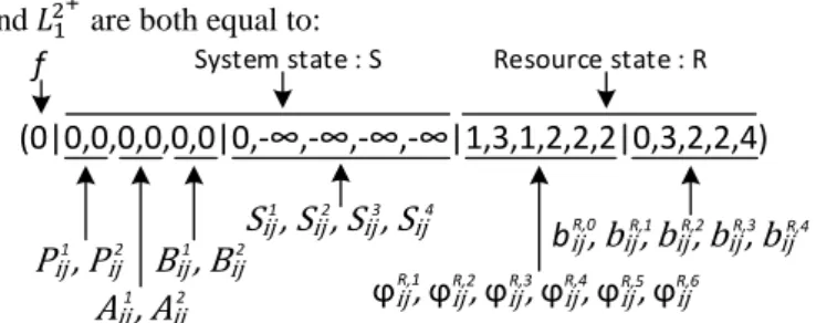
For the first step (Fig. 8), the graph is initialized with a label 𝐿#

leading to two labels stored on node 1+ _{and 2}+_{, corresponding}

to activity 0 as 𝜆(1+_{) = 0 and 𝜆(2}+_{) = 0. The two labels 𝐿} 1 1+

and 𝐿12+ are both equal to:

System state : S Resource state : R

f

P

, P

A

, A

B

, B

S

, S

, S

, S

(0|0,0,0,0,0,0|0,-∞,-∞,-∞,-∞|1,3,1,2,2,2|0,3,2,2,4)

ϕ

, ϕ

, ϕ

, ϕ

, ϕ

, ϕ

b

, b

, b

, b

, b

with respect to the label definition, 𝑖 = 1 and 𝑗 = {1+_{, 2}+_{}. The}

9 0 2 (1,2) 1+ 1

-L

-1

-4

1

-1

L

#

L

Figure 8. Initialization of the graph 𝑇𝜑( 𝑈, 𝑉, 𝐸, 𝐹).

In the second step, the node number 2+ is removed from the queue and all the labels on node 2+ _{are propagated on node 2}−_.

In this step, two labels are created (Fig. 9):

 𝐿12−= (2|1,0,2,0,2,0|0,2, −∞, −∞, 4|1,0,1,2,2,2|0,0,2,2,4)  𝐿22 − = (2|0,1,0,2,0,2|0,2, −∞, −∞, 4|1,1,1,2,2,2|0,1,2,2,4)

0

1

L

2

1

_L

2

-1

L

2

-2

Figure 9. Step 2: Propagation of the label on arc number 2 in

𝑇𝜑_{( 𝑈, 𝑉, 𝐸, 𝐹).}

The creation of label 𝐿21

−

can be designed to take label 𝐿12

+

, the arc (0,1) with the information (3,2) and the assignment of vehicle 1 into account.

Label 𝐿2₁− is created considering the propagation rule (loaded transport operation): 𝑃1,21−= 𝜆(2−) = 1 𝐴1,21 −= 𝐵_1,21 ++ 𝑡0,1= 0 + 2 = 2 𝐵1,21 −= 𝐴_1,21 −= 2 𝑆1,21 −= 𝑚𝑎 𝑥(𝑆_1,21 +; 𝐴_1,21 −) = 𝑚𝑎 𝑥(−∞; 2) = 2 𝜑1,2𝑅,2 −= 𝜑_1,2𝑅,2 +− 𝑚 𝑖𝑛( 𝜑_1,2𝑅,2+; 𝑐1) = 3 − 𝑚𝑖𝑛(2; 3) = 0 𝑏1,2𝑅,1− = 𝑏_1,2𝑅,1+ − 𝑚 𝑖𝑛( 𝜑_1,2𝑅,2+; 𝑐1) = 3 − 𝑚𝑖𝑛(2; 3) = 0

and because 𝑏_1,2𝑅,1− = 0, the earliest starting time of all successors

of activity 1 should be updated: 𝑆1,2∗ −= 𝑆1,21 −+ 𝑝1= 2 + 2 = 4

The two labels created are not comparable due to the position of the vehicles. They are therefore both stored on node 2−. The queue is updated and is equal to Λ = [1+_{, 2}−_].

In the third step, the node number 2− _{is removed from the queue}

and the labels on node 2− _{are propagated on nodes 1}+_{, 2}+_{, 3}+_{, 4}+

with a feasibility check. This label propagation concerns unloaded transport operations in the dashed arcs in Fig. 8.

Ten labels are created:

 Four on node 1+_: 𝐿11 + = (4|0,0,4,0,4,0|0,2, −∞, −∞, 4|1,0,1,2,2,2|0,0,2,2,4) 𝐿12 + = (2|1,0,2,0,2,0|0,2, −∞, −∞, 4|1,0,1,2,2,2|0,0,2,2,4) 𝐿13 + = (2|0,1,0,2,0,2|0,2, −∞, −∞, 4|1,1,1,2,2,2|0,1,2,2,4) 𝐿14 + = (4|0,0,0,4,0,4|0,2, −∞, −∞, 4|1,1,1,2,2,2|0,1,2,2,4)  Two on node 2+_: 𝐿21+= (2|0,1,0,2,0,2|0,2, −∞, −∞, −∞|1,1,1,2,2,2|0,1,2,2,4) 𝐿22+= (4|0,0,0,4,0,4|0,2, −∞, −∞, −∞|1,1,1,2,2,2|0,1,2,2,4)  Two on node 3−_: 𝐿31 + = (4|1,0,2,0,4,0|0,2, −∞, −∞, 4|1,0,1,2,2,2|0,0,2,2,4) 𝐿32 + = (4|1,1,2,2,2,4|0,2, −∞, −∞, 4|1,0,1,2,2,2|0,0,2,2,4)  Two on node 4−_: 𝐿41 + = 𝐿13 + and 𝐿42 + = 𝐿23 + Table 3

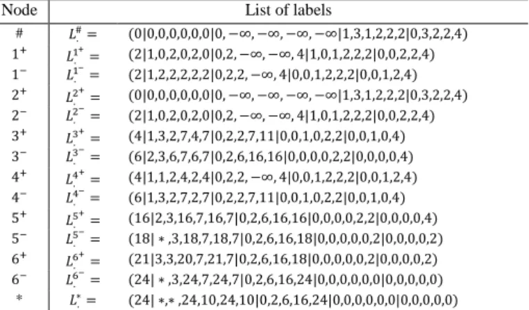
Details of all the labels of the optimal solution in Fig. 10.

Node List of labels

# 𝐿#. = (0|0,0,0,0,0,0|0, −∞, −∞, −∞, −∞|1,3,1,2,2,2|0,3,2,2,4) 1+ _𝐿 . 1+ = (2|1,0,2,0,2,0|0,2, −∞, −∞, 4|1,0,1,2,2,2|0,0,2,2,4) 1− _𝐿 . 1− = (2|1,2,2,2,2,2|0,2,2, −∞, 4|0,0,1,2,2,2|0,0,1,2,4) 2+ _𝐿 . 2+ = (0|0,0,0,0,0,0|0, −∞, −∞, −∞, −∞|1,3,1,2,2,2|0,3,2,2,4) 2− _𝐿 . 2− = (2|1,0,2,0,2,0|0,2, −∞, −∞, 4|1,0,1,2,2,2|0,0,2,2,4) 3+ _𝐿 . 3+ = (4|1,3,2,7,4,7|0,2,2,7,11|0,0,1,0,2,2|0,0,1,0,4) 3− _𝐿 . 3− = (6|2,3,6,7,6,7|0,2,6,16,16|0,0,0,0,2,2|0,0,0,0,4) 4+ _𝐿 . 4+ = (4|1,1,2,4,2,4|0,2,2, −∞, 4|0,0,1,2,2,2|0,0,1,2,4) 4− _𝐿 . 4− = (6|1,3,2,7,2,7|0,2,2,7,11|0,0,1,0,2,2|0,0,1,0,4) 5+ _𝐿 . 5+ = (16|2,3,16,7,16,7|0,2,6,16,16|0,0,0,0,2,2|0,0,0,0,4) 5− _𝐿 . 5− = (18| ∗ ,3,18,7,18,7|0,2,6,16,18|0,0,0,0,0,2|0,0,0,0,2) 6+ _𝐿 . 6+ = (21|3,3,20,7,21,7|0,2,6,16,18|0,0,0,0,0,2|0,0,0,0,2) 6− _𝐿 . 6− = (24| ∗ ,3,24,7,24,7|0,2,6,16,24|0,0,0,0,0,0|0,0,0,0,0) * 𝐿∗.= (24| ∗,∗ ,24,10,24,10|0,2,6,16,24|0,0,0,0,0,0|0,0,0,0,0)

At the end of the algorithm, i.e., when all labels have been propagated (the queue Λ is then empty), a set of non-dominated solutions are obtained. The final solutions that minimize the makespan are optimal since they minimize the objective function (first parameter in the labels). An optimal solution (solution minimizing the makespan) is introduced in Fig. 10 considering the trip of vehicle 1 in Fig. 10.a and the trip of vehicle 2 in Fig. 10.b. All the labels are fully described in Table 3. In Fig. 1 and 2,

an extended Gantt diagramdisplays this optimal solution.

2.5. Discussion

The algorithm proposed to solve the RCPSPR from a flow solution takes advantage of a resource-constrained shortest path algorithm.

This algorithm is dedicated to the resolution of an arc routing problem with specific features based on the fact that the

10 scheduling and the routing are interrelated with shared resource

management. In the problem of interest here, the transport operations are first linked by precedence constraints due to the flow definition and, second, model the required arcs with a quantity that can eventually exceed the vehicle capacity. To the best of our knowledge, there is no specific method in the arc routing community that simultaneously tackles these constraints

and that could provide time-saving implementation.

This algorithm first attempts to optimally transform a RCPSP flow solution into a RCPSPR solution and is the first step towards defining an efficient framework based on the indirect modeling of solutions using the flow. This is a theoretical contribution with a practical application.

(0,0) 0 2 1+ 1 -1 2 (1,2) 3 -1 3 4+ 4 -2 4 5+ 5 -4 3 (2,3) 6+ 6 -0 1 (3,2) 2+ 2 -(2,2) * # (0,0) 3+ (0,3) (0,2,2)

L

_.

L

_.

-L

_.

L

_.

-L

_.

L

_.

-L

_.

L

_.

-L

_.

L

_.

-L

_.

L

_.

L

_.

-L

_.

Figure 10. Representation of the two trips of an optimal solution on the graph 𝑇𝜑( 𝑈, 𝑉, 𝐸, 𝐹). 3. Numerical experiments

The aim of these experiments is to provide feedback on the efficiency of the algorithm to compute an optimal RCPSPR solution from one RCPSP solution. The efficiency is analyzed considering the CPU time required in practice and the total number of labels generated during the process.

All experiments were carried out on a single thread C program, using Visual Studio and a Windows 7 operating system on a Dell Optiflex9020 with an Intel Core i7-4770 CPU 3.4 GHz and 16 Gb of RAM, meaning approximately 2671 Mflops (see Dongarra et al., 2014). The CPLEX experiments were carried out on the same computer. In order to ensure fair future comparative studies, all results and one example are available at the following web page:

http://fc.isima.fr/~vinot/Research/RCPSPR_Flow.html

3.1. New set of instances

To the best of our knowledge, no instance dealing with this problem is available. Consequently, numerical experiments are based on a new set of small-scale instances composed of 18 instances with six activities (plus the dummy nodes). In these instances, the location of the activities can be divided into two configurations: the first one with a uniform distribution of the activities and the second one with two clusters.

Tables 4 and 5 introduce the number of activities to be scheduled, but this number does not include information on the number of transport operations. The number of transport operations depends on the flow modeling a RCPSP solution and on the vehicle capacities. Column 𝐿𝐵(𝑛) is the lower bound of the total number of operations to be scheduled, considering both 𝑛 and the minimal number of arcs with a non-null flow, i. e., 𝑛 + 1, obtained with an ordered sequence of activities.

11

Table 4

Small-scale instance characteristics.

Instances n LB(n) Location _requirement Resource _availability Resource _capacity Vehicle Ratio

LMQV_U1 6 13 uniform {4;10;3;3;8;4} 12 {12;12} 1.6 LMQV_U2 6 13 uniform {4;10;3;3;8;4} 12 {12;12} 1.1 LMQV_U3 6 13 uniform {4;10;3;3;8;4} 12 {12;12} 1.3 LMQV_U4 6 13 uniform {2;8;7;8;8;5} 14 {6;5} 0.5 LMQV_U5 6 13 uniform {2;8;7;8;8;5} 14 {6;5} 0.4 LMQV_U6 6 13 uniform {2;8;7;8;8;5} 14 {6;5} 0.4 LMQV_U7 6 13 uniform {5;3;8;2;3;1} 10 {4;2} 0.3 LMQV_U8 6 13 uniform {5;3;8;2;3;1} 10 {4;2} 0.3 LMQV_U9 6 13 uniform {5;3;8;2;3;1} 10 {4;2} 0.3 LMQV_C1 6 13 clusters {7;7;5;7;5;4} 7 {7;7} 3.0 LMQV_C2 6 13 clusters {7;7;5;7;5;4} 7 {7;7} 2.1 LMQV_C3 6 13 clusters {7;7;5;7;5;4} 7 {7;7} 3.0 LMQV_C4 6 13 clusters {7;1;2;6;2;6} 11 {6;5} 1.1 LMQV_C5 6 13 clusters {7;1;2;6;2;6} 11 {6;5} 1.0 LMQV_C6 6 13 clusters {7;1;2;6;2;6} 11 {6;5} 1.0 LMQV_C7 6 13 clusters {4;10;4;6;3;4} 12 {4;2} 0.8 LMQV_C8 6 13 clusters {4;10;4;6;3;4} 12 {4;2} 0.8 LMQV_C9 6 13 clusters {4;10;4;6;3;4} 12 {4;2} 0.8

The resource requirement and availability, the capacity of the vehicles and the ratio are given in Table 4. The ratio is defined as the ratio between the average duration of an activity and the average duration of a transport operation per vehicle, which is representative of the relative importance of the scheduling vs. the routing. A ratio greater than one means that the scheduling processing time represents a greater amount of time than the routing, and a ratio lower than one implies the reverse.

A new set of medium-scale instances composed of nine instances with 30 activities (plus the dummy nodes) is also introduced. In these instances, the location of the activities is divided into three configurations: the first one with a uniform distribution of the activities and the depot located at the center of the location, the second one with two clusters and the depot located at the center of the location, and the third one with two clusters and the depot location in a cluster (Table 5).

Due to the combinatorial nature of the RCPSP, obtaining optimal solutions using exact methods for problems with over 60 or so activities becomes intractable and, hence, impractical (Valls et al., 2005). Moreover, the RCPSPR is an extension of the RCPSP with the management of a fleet of vehicles where the decision variables encompass both RPCSP variables and a set of variables for the routing problem. In this new set of medium instances, more than 60 operations have to be scheduled (𝐿𝐵(𝑛) = 61). The optimal resolution of this set of instances is challenging due, first, to the large number of operations to be scheduled, including both the activities and the transport operations and, second, to the coordination between the activities and the transport operations, including the assignment of vehicles to the transport operations.

All the details of the instances are available at the web page.

Table 5

Medium-scale instance characteristics.

Instances n LB(n) Location Resource

requirement Resource availability Vehicle capacity Ratio LMQV_J30_U1 30 61 uniform [1;10] 13 {13;13} 0.7 LMQV_J30_U2 30 61 uniform [1;10] 14 {8;6} 0.3 LMQV_J30_U3 30 61 uniform [1;10] 13 {13;9} 1.0 LMQV_J30_C1 30 61 clusters [1;10] 15 {15;15} 0.8 LMQV_J30_C2 30 61 clusters [1;10] 11 {7;5} 0.3 LMQV_J30_C3 30 61 clusters [1;10] 12 {12;9} 0.9 LMQV_J30_CC1 30 61 clusters [1;10] 13 {13;13} 0.6 LMQV_J30_CC2 30 61 clusters [1;10] 14 {8;6} 0.3 LMQV_J30_CC3 30 61 clusters [1;10] 13 {13;8} 1.1

3.2. Performance of the shortest path algorithm

The effectiveness of the shortest path algorithm can be evaluated on small-scale instances by considering a restriction of 𝑌𝑖 to 500

labels per node, with 𝑟 = 10 replications per instance. One replication models one randomly generated flow (with one replication considering the flow leading to the optimal RCPSP solution). The shortest path algorithm is compared to an optimal resolution with IBM ILOG CPLEX 12.6 and a linear formulation of the problem (Lacomme et al., 2017).

For each instance, ℎ𝐶(𝑥, r) defines the average solution cost with

CPLEX, and 𝑡𝐶(𝑥, 𝑟) the average computational time required to

find the optimal solution with CPLEX. Similarly, ℎ𝑆𝑃(𝑥, r)

denotes the average best-found solution cost using the shortest path algorithm (restriction of 𝑌_𝑖 can lead to a suboptimal solution), and 𝑡𝑆𝑃(𝑥, 𝑟) the average resource-constrained shortest

path algorithm time to the best-found solution. The notation 𝑔(𝑥, 𝑛) denotes the gap between ℎ𝑆𝑃(𝑥, 𝑟) and ℎ𝐶(𝑥, 𝑟) for the

instance 𝑥, and 𝑔(𝑥, 𝑟) is an estimation of the average gap considering 𝑛 replications. The number of optimal solutions

12

found by the shortest path algorithm for the instance 𝑥 with 𝑛

replications is denoted 𝑛𝑆𝑃(𝑥, 𝑛). Let us denote 𝑔(. , 𝑟) as the

estimation of the average gap considering the 18 instances, 𝑡∗(. , 𝑟) (resp. 𝑡𝑆𝑃(. , 𝑟), and 𝑡𝐶(. , 𝑟)) the estimation of the average

computational time (resp. of CPLEX and of the shortest path), 𝑛𝑆𝑃(. , 𝑟) the average number of optimal solutions found over the

18 instances, and 𝑛𝑆𝑃(. , . ) = ∑𝑥=18𝑥=1 𝑛𝑆𝑃(𝑥, 𝑟), i.e., the total number

of optimal solutions found during the 10 replications and the 18 instances.

The average resource-constrained shortest path computational time 𝑡𝑆𝑃(. , 𝑟) in Table 6 is approximately 8.2 seconds,

approximately two times lower that the CPLEX computational time 𝑡𝐶(. , 𝑟), which is approximately 17.8 seconds (Table 6). The

average number of optimal solutions found by the resource-constrained shortest path algorithm is greater than 9.9, which means that the percent of optimal solutions found is close to 100%. It can be observed that the resource-constrained shortest path algorithm finds the optimal solution for 176 flows out of 180 (𝑛𝑆𝑃(. , . )), with an average gap of 0.04%.

Table 6

Average shortest path efficiency with a restriction of 𝑌𝑖 to 500 labels per node (𝑟 = 10 flows per instance) for small-scale instances.

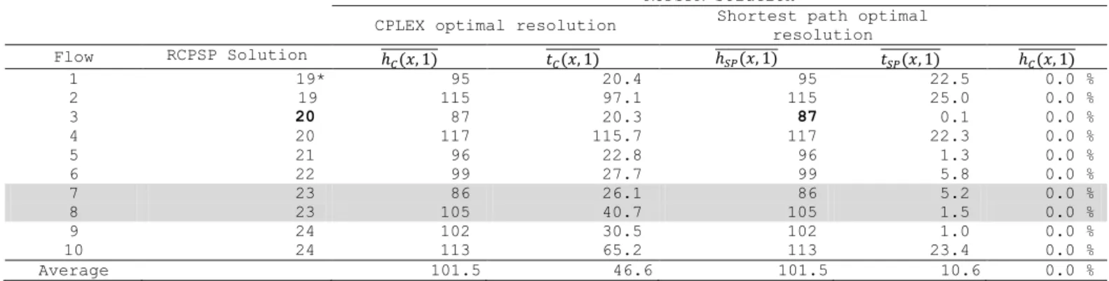
CPLEX optimal resolution Shortest path optimal resolution Instances _{ℎ𝐶(𝑥, r) 𝑡𝐶(𝑥, 𝑟)} ̅̅̅̅̅̅̅̅̅̅̅ ℎ𝑆𝑃(𝑥, r) 𝑛𝑆𝑃(𝑥, 𝑟) 𝑡𝑆𝑃(𝑥, 𝑟) 𝑔(𝑥, 𝑟) LMQV_U1 101.5 46.6 101.5 10/10 10.6 0.00 % LMQV_U2 198.5 37.2 198.7 9/10 10.2 0.09 % LMQV_U3 246.6 29.0 246.6 10/10 11.9 0.00 % LMQV_U4 123.3 31.0 123.3 10/10 3.6 0.00 % LMQV_U5 247.1 32.3 247.1 10/10 4.3 0.00 % LMQV_U6 288.1 34.5 288.1 10/10 7.0 0.00 % LMQV_U7 128.4 9.9 128.4 10/10 2.2 0.00 % LMQV_U8 261.1 9.3 261.1 10/10 2.4 0.00 % LMQV_U9 276.1 9.2 276.1 10/10 2.5 0.00 % LMQV_C1 78.6 11.1 78.6 10/10 0.0 0.00 % LMQV_C2 135.6 9.0 135.6 10/10 0.0 0.00 % LMQV_C3 160.6 10.0 160.6 10/10 0.0 0.00 % LMQV_C4 45.2 10.5 45.3 9/10 21.1 0.20 % LMQV_C5 92.0 12.2 92.3 9/10 25.8 0.28 % LMQV_C6 94.6 12.2 94.8 9/10 24.6 0.19 % LMQV_C7 66.4 5.6 66.4 10/10 6.3 0.00 % LMQV_C8 132.6 5.2 132.6 10/10 10.2 0.00 % LMQV_C9 136.7 5.7 136.7 10/10 5.2 0.00 % 𝑔(. , 𝑟) 0.04 % 𝑡_∗(. , 𝑟) 17.8 8.2 𝑛𝑆𝑃(. , 𝑟) 9.99 𝑛_𝑆𝑃(. , . ) 176/180 Table 7

RCPSP/RCPSPR solutions (instance LMQV_U1).

RCPSPR Solution

CPLEX optimal resolution Shortest path optimal resolution Flow RCPSP Solution _ℎ 𝐶(𝑥, 1) 𝑡𝐶(𝑥, 1) ℎ̅̅̅̅̅̅̅̅̅̅̅ 𝑆𝑃(𝑥, 1) 𝑡𝑆𝑃(𝑥, 1) ℎ𝐶(𝑥, 1) 1 19* 95 20.4 95 22.5 0.0 % 2 19 115 97.1 115 25.0 0.0 % 3 20 87 20.3 87 0.1 0.0 % 4 20 117 115.7 117 22.3 0.0 % 5 21 96 22.8 96 1.3 0.0 % 6 22 99 27.7 99 5.8 0.0 % 7 23 86 26.1 86 5.2 0.0 % 8 23 105 40.7 105 1.5 0.0 % 9 24 102 30.5 102 1.0 0.0 % 10 24 113 65.2 113 23.4 0.0 % Average 101.5 46.6 101.5 10.6 0.0 %

Table 7 gives the set of flows randomly generated for instance LMQV_U1 (that include the optimal RCPSP flow) and provides the optimal RCPSP solution (column 2) for each flow and the optimal RCPSPR solutions provided by CPLEX and by the shortest path algorithm. The set of 10 flows introduced in Table 7 encompasses the flow of the optimal RCPSP solution. Note that the best (optimal) solution of the RCPSP has a cost equal to 19, whereas the worst one in Table 7 has a cost equal to 24. Nevertheless, the best solution found for the RCPSPR has a cost equal to 87 and was obtained with a solution of the RCPSP with

a cost equal to 20 (flow number 3 in Table 7). Such results lead us to consider that high-quality solutions of the RCPSP do not lead to high-quality RCPSPR solutions, which is not really surprising since there is no reason that a quality solution for one sub-problem favors the computation of a quality solution for the whole problem. Indeed, several solutions of the RCPSP with the same makespan (for example, 23) could lead to very different solutions of the RCPSPR with a cost ranging from 86 to 105. Such behavior suggests that it would be difficult to devise a rule

13 that could provide quality RCPSPR solutions by considering the

quality RCPSP solutions.

Table 8

Shortest path for 𝑟 = 1 flow on each medium-scale instance.

Shortest path optimal resolution (NL=50)

Instances n 𝑛𝜑 RCPSP Solution ℎ̅̅̅̅̅̅̅̅̅̅̅ 𝑆𝑃(𝑥, 1) 𝑡𝑆𝑃(𝑥, 1) LMQV_J30_U1 30 56 96 250 80.4 LMQV_J30_U2 30 57 105 276 697.0 LMQV_J30_U3 30 50 82 129 5.3 LMQV_J30_C1 30 53 113 221 729.0 LMQV_J30_C2 30 56 81 231 336.9 LMQV_J30_C3 30 57 83 139 32.9 LMQV_J30_CC1 30 60 103 271 270.3 LMQV_J30_CC2 30 58 108 270 305.6 LMQV_J30_CC3 30 58 100 158 89.9 𝑡∗(. , 𝑛) 283.0

Table 8 reports the results obtained by the resource-constrained shortest path algorithm with a restriction of 𝑌_𝑖 to 50 labels per node, with 𝑟 = 1 replication per instance. In Table 8, the cost of the RCPSP solution associated with the flow is reported in column 4. Unfortunately, the best-found solution of the algorithm cannot be compared to a solution obtained with CLEX. With 30 activities, the linear formulation remains intractable due the huge numbers of both variables and constraints, including binary variables. For example, it should be noted that the instance LMQV_J30_U1 cannot be solved to optimality in 2 days of computational time using CPLEX.

For the couples instance/flow introduced in Table 8, a lower bound of the number of transport operations is provided in

column 𝑛_𝜑. For the instance LMQV_J30_CC1, we have 30

activities plus at least 60 transport operations, representing a total of 90 operations to be scheduled, assuming that each flow is transferred by one vehicle only with one transport. The minimal number of transport operations (with a value of 60) is induced by arcs with a non-null flow.

3.3. Performance of the label management rules

To evaluate the efficiency of the algorithm, no restriction of 𝑌𝑖,

i.e., all labels that are required to be kept, is stored on nodes, and Table 9 provides the number of:

 labels inserted on the node due to the 𝐼𝑁𝑆𝐸𝑅𝑇_𝐿𝐴𝐵𝐸𝐿()

function;

 labels pruned on the node with 𝐶𝐻𝐸𝐶𝐾_𝑈𝐵_𝐿𝐵() function;

 labels deleted on the node with 𝐴𝑃𝑃𝐿𝑌_𝐷𝑂𝑀𝐼𝑁𝐴𝑁𝐶𝐸() function.

All experiments were carried out on the 18 small-scale instances considering the 10 replications previously used, and the following notations are used in Table 9:

 𝑇𝑁𝐿𝐺(𝑥, 𝑗) Total number of labels generated during the

replication number 𝑗;

 𝑇𝑁𝐿𝐺(𝑥, 𝑟) Average number of labels generated during

the 𝑟 replications;

 𝑇𝑁𝐿𝑃(𝑥, 𝑟) Average number of labels pruned per instance

𝑥

during the 𝑟 replications;

 𝑃𝑝(𝑥, 𝑗) Percent of labels pruned considering

𝑇𝑁𝐿𝐺(𝑥, 𝑗);

 𝑃𝑝(𝑥, 𝑟) Average percent of labels pruned with

𝑃𝑝(𝑥, 𝑟) = 𝐴𝑣𝑔𝑗=1,𝑟(𝑃𝑝(𝑥, 𝑗)) ;

 𝑇𝑁𝐿𝐷(𝑥, 𝑟) Total number of labels dominated;

 𝑃𝑑(𝑥, 𝑗) Percent of labels discarded thanks to the

domination rule considering 𝑇𝑁𝐿𝐺(𝑥, 𝑗);

 𝑃𝑑(𝑥, 𝑟) Average percent of labels discarded, with

𝑃𝑝(𝑥, 𝑟) = 𝐴𝑣𝑔𝑗=1,𝑟(𝑃𝑝(𝑥, 𝑗)) ;

 𝑃(. , . ) Average percent of 𝑃𝑝(𝑥, 𝑟) or 𝑃𝑑(𝑥, 𝑟) for all

instances;

 𝐴𝑣𝑔(. , . ) Average number of labels generated, pruned

14

Table 9

Efficiency of the label management rules with 𝑍𝑖= 𝑌𝑖 for small-scale instances.

Instances 𝑇𝑁𝐿𝐺(𝑥, 𝑟) 𝑇𝑁𝐿𝑃(𝑥, 𝑟) 𝑇𝑁𝐿𝐷(𝑥, 𝑟) 𝑃𝑃(𝑥, 𝑟) 𝑃𝑑(𝑥, 𝑟) LMQV_U1 256 514.9 49 313.8 114 201.4 19.2 44.5 LMQV_U2 245 631.8 47 122.1 111 452.6 19.2 45.4 LMQV_U3 298 695.6 57 901.4 136 189.4 19.4 45.6 LMQV_U4 124 521.7 21 261.5 64 856.7 17.1 52.1 LMQV_U5 134 996.0 22 109.0 73 049.9 16.4 54.1 LMQV_U6 198 907.8 28 581.2 112 077.0 14.4 56.3 LMQV_U7 177 200.4 40 449.2 78 194.4 22.8 44.1 LMQV_U8 189 100.6 42 760.4 84 848.8 22.6 44.9 LMQV_U9 217 710.7 51 939.6 92 055.1 23.9 42.3 LMQV_C1 4.4 2.8 0.0 63.6 0.0 LMQV_C2 4.4 2.8 0.0 63.6 0.0 LMQV_C3 4.4 2.8 0.0 63.6 0.0 LMQV_C4 543 915.1 101 480.3 267 705.7 18.7 49.2 LMQV_C5 589 227.4 107 571.8 281 184.5 18.3 47.7 LMQV_C6 580 233.6 107 110.3 280 699.6 18.5 48.4 LMQV_C7 230 693.0 26 232.9 167 281.8 11.4 72.5 LMQV_C8 294 602.6 35 820.0 203 370.0 12.2 69.0 LMQV_C9 273 935.0 33 845.2 187 245.9 12.4 68.4 𝐴𝑣𝑔(. , . ) 241 994.4 42 972.6 125 255.8 𝑃(. , . ) 25.4 43.6

The following remarks hold:

 25% of the labels generated are pruned (thanks to the function 𝐶𝐻𝐸𝐶𝐾_𝑈𝐵_𝐿𝐵(𝐿, 𝐿𝐵, 𝑈𝐵));

 43% of the labels generated are deleted (thanks to the

dominance rule with 𝐷𝑂𝑀𝐼𝑁𝐴𝑇𝐸(𝑖, 𝑗) and

𝐴𝑃𝑃𝐿𝑌_𝐷𝑂𝑀𝐼𝑁𝐴𝑁𝐶𝐸(𝐿, 𝑍).

These results lead us to consider that the dominance rule we introduced is highly efficient and defines the cornerstone of the shortest path algorithm.

3.4. Remarks

The results first confirm the algorithm efficiency from a computational point of view and prove that the algorithm can be used in practice and could be integrated into an iterative metaheuristic-based search on an indirect representation of solutions (Cheng et al., 1996) (Prins, 2002). The resource-constrained shortest path algorithm can be used to determine an evaluation function that defines the optimal RCPSPR solution for one flow. From this point of view, the computational efficiency of the method is crucial. Intensive numerical experiments have shown that the algorithm can be adapted depending on the context, and should make it possible to find quality RCPSPR solutions within an acceptable computational time. An experiment based on 18 flows revealed that the computational time can be reduced to 15 seconds with 500 labels per node, and to 0.4 seconds with 50 labels per node, providing the optimal RCPSPR solution in 67% of the flows (the average deviation to the optimal solution is less than 0.9%). Because the evaluation function that makes it possible to associate a flow with a solution can be a part of a global optimization process, the capacity of the algorithm to ensure quasi-optimal evaluation in a very short computational time is a significant highlight of the algorithm.

4. Concluding remarks

A new resource-constrained shortest path algorithm is introduced to define a RCPSPR solution from one RCPSP flow solution. The

RCPSPR is a new integrated problem dealing with scheduling and routing based on the RCPSP to which routing constraints with a heterogeneous fleet of vehicles with limited capacities have been added.

Our contribution concerns: (1) the label definition that encompasses both system state and resources; (2) the dominance rule; (3) the propagation rule.

The algorithm ensures an efficient algorithmic solution to deal with a proper coordination between scheduling and routing problems since it points the way towards a definition of an iterative search process based on an indirect representation by an efficient computation of RCPSP solutions from a flow of the RCPSP. It should be noted that the resource-constrained shortest path algorithm we have introduced is a new way to solve arc routing problems by shortest path computation.

Acknowledgements: This work was carried out and funded within the framework of the ATHENA project (Reference: ANR-13-BS02-0006) and the Labex MS2T. It was supported by the French government through the “Investments for the future" program managed by the French National Research Agency (Reference: ANR-11-IDEX-0004-02).

References

Adnen E.A., Mohsen E. An efficient new heuristic for the hoist scheduling problem. Computers & Operations Research 2016; 67: 184-192.

Afsar H.M., Lacomme P., Ren, L., Prodhon C., Vigo, D. Resolution of a Job-Shop problem with transportation constraints: a master/slave approach. IFAC 2016; 49(12): 898-903.

Alvarez-Valdés R., Tamarit J.M. The project scheduling prolyhedron: Dimension, facets and lifting theorems. European Journal of Operational Research 1993; 67: 204-220.

Artigues C., Michelon P., Reusser S. Insertion for static and dynamic RCPSP. European Journal of Operational Research 2003; 149: 249-67.

Caumond A., Lacomme P., Moukrim A., Tchernev N. An MILP for scheduling problems in a FMS with one vehicle. European Journal of Operational Research 2009; 199(3): 706-722.

Cheng, R., Gen, M. Tsujimura, Y. A tutorial survey of job-shop scheduling problems using genetic algorithms – I representation. Computers and Industrial Engineering 1996; 30: 983–997.