Compensation of incoherent errors in the precise implementation of effective Hamiltonians for quantum information processing

Compensation of Incoherent Errors in the Precise

Implementation of Effective Hamiltonians for Quantum

Information Processing

by

Amro M. Farid

S.B. Mechanical Engineering

Massachusetts Institute of Technology 2000

Submitted to the Mechanical Engineering

MASSACHUSETTS _INSTITUTE OF TECHNOLOGY

OCT 2 5 2002

LIBRARIES

in partial fulfillment of the requirements for the degree of

Master of Science in Mechanical Engineering

at the

MASSACHUSETTS INSTITUTE OF TECHNOLOGY

June 2002

©

Massachusetts Institute of Technology 2002. All rights reserved.

Author...

Mechanical Engineering

May 21, 2002

Certified by ...

C ertified by ...

Seth Lloyd

P

sor of Mechanical Engineering

.

ks Supervisor

D

ory

Professor of Nuclear ngineering

Thesis Supervisor

A ccepted by ...-

% . .

...

Ain Sonin

Chairman, Department Committee on Graduate Students

Compensation of Incoherent Errors in the Precise Implementation of

Effective Hamiltonians for Quantum Information Processing

by

Amro M. Farid

Submitted to the Mechanical Engineering on May 21, 2002, in partial fulfillment of the

requirements for the degree of

Master of Science in Mechanical Engineering

Abstract

This thesis sets out to present an algorithm for compensation of incoherent errors in quan-tum information processing (QIP). In particular, it addresses the incoherent errors that arise from RF inhomogeneity in a liquid state NMR system. It briefly describes NMR's place in QIP experimental developments and explains the need to eliminate the errors in-troduced by RF inhomogeneity. An algorithm for compensation is proposed provided that one has prior knowledge of the system Hamiltonian and a measurement of the degree of RF inhomogeneity. The algorithm was used to create two sets of RF pulses; an uncompensated set that did not use the RF inhomogeneity measurement and a more robust set that did use the measurement. Simulation results indicate that all of the new pulses reduced the error by approximately an order of magnitude for the measured RF inhomgeneity, as well as for most other types of RF inhomogeneity. This result was verified in experiment, where correlations were improved by 0.024 on average. In total, errors due to RF inhomogeneity were reduced by a factor of six.

Thesis Supervisor: Seth Lloyd

Title: Professor of Mechanical Engineering Thesis Supervisor: David Cory

Acknowledgments

I would like to thank Professors David Cory and Seth Lloyd for exposing me to the new and exciting field of Quantum Information Processing. Their combined knowledge of the field has gone a long way to further my understanding and illuminate particularly difficult concepts. This project has also broadened my understanding of control theory, signals and systems, quantum mechanics, and electromagnetism. It has been a tremendous opportunity to work within Professor Cory's laboratory which has provided the spectrometers and the computers required for this research. Lastly, I would like to thanks Professors Cory and Lloyd for academically and professionally advising me over the last two years.

I would also like to thank Marco Pravia for our combined efforts on this project. He has made great efforts within the same field which have helped me greatly in the completion of this thesis. I would like to thank especially Evan Fortunato, Greg Boutis, Grum Tekle-mariam, and Yaakov Weinstein for many stimulating conversations over the last two years. Especially during my first year, they have often taken the time to impart their knowledge to me as well as other less senior members of the research group. I also would like to thank the other members of the group for providing a very helpful and cooperative work environment. Many people in my personal life have helped me in producing this document. First, I must thank Paula Deardon. With respect to my MIT life, she has provided unquestionable moral support and encouragement, even during the most trying times of the last two years. I also thank Jan Meyer for encouragement over the last year and a half. Finally, I thank my family. Even from New York, my twin sister, Nora has an amazing sense to know when I most need support. Sarah's comical anecdotes of middle school life lighten even the most stressful days. My mother, Yomn Elsayed is just always there. Lastly, I thank my father Mohsen Farid for sparking my interest in physics at a very young age and encouraging me to continue with it for graduate study.

Contents

1 Introduction 8

1.1 Background on QIP . . . . 8

1.2 NMR as a paradigm for QIP . . . . 9

1.3 Experimental Apparatus . . . . 9

1.4 Motivation for Robust Control . . . . 10

1.5 Overview of Approach . . . . 11

2 Dynamics of Liquid State Nuclear Magnetic Resonance 13 2.1 Spin Wavefunctions, Operators, and Bra-Kets . . . . 13

2.2 A Spin 1/2 Particle in the Static Magnetic Field . . . . 15

2.3 Thermal Excitation and the Density Matrix . . . . 15

2.4 The External Hamiltonian and the Rotating Frame . . . . 16

2.5 Multiple Qubit Molecules and the Spin-Spin Scalar J coupling . . . . 17

3 A Method for Compensating for Incoherent Errors 20 3.1 Incoherent Errors in Quantum Control . . . . 20

3.2 A Brief Review of Compensation for RF Inhomogeneity . . . . 23

3.3 An Method for Compensation . . . . 23

3.3.1 Experimental Determination of RF Inhomogeneity . . . . 23

3.3.2 Optimization Algorithm . . . . 24

3.4 Summary of Pulse Parameters . . . . 28

3.5 Simulated Robustness to RF Inhomogeneity . . . . 28

4.2 State and Process Tomography . . . . 32

4.3 Experimental Results . . . . 34

4.4 Degree of Improvement in RF Inhomogeneity Compensation . . . . 35

5 Discussion 36 5.1 Further Aspects of Pulse Performance . . . . 36

5.2 Pulse Fidelity in the Presence of Temporally Incoherent Errors . . . . 37

5.3 Exploring Achievable Fidelities . . . . 38

5.4 Further Applications of Algorithm . . . . 39

6 Conclusions and Recommendations 41 6.1 Conclusions . . . . 41

6.2 Recommendations . . . . 41

A List of Variables 42

B Robust Pulse Parameters 45

List of Figures

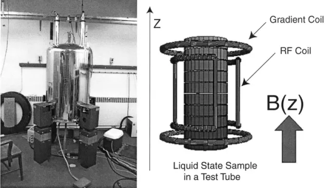
1-1 On the left is a photo of a 9.6T magnet. On the right, is a diagram of the RF coil that applies time varying magnetic fields to the sample within. . . 10 1-2 A schematic diagram of the RF coil's dual function; external control of the

spin system and signal detection [18] . . . . . 11 2-1 A Graphical Representation of the Alanine Molecule. At the bottom right,

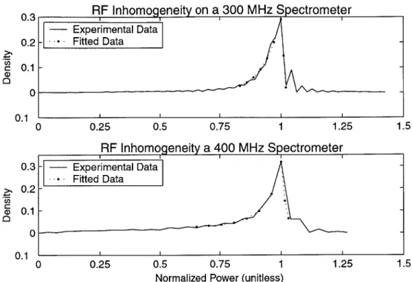
the chemical shift frequencies and the scalar coupling strengths are shown in units of H z. . . . . 17 3-1 On the 300MHz spectrometer, the width of the density function at half the

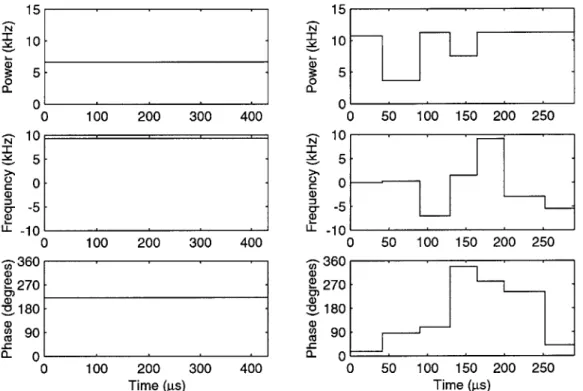
maximum value was 6.23 percent. Similarly, the 400 MHz spectrometer had a width of 7.00 percent. Integrating over the density functions yields an average delivered power attenuated by 3.50 and 5.64 percent respectively. . 25 3-2 On the left is a an initial guess of the optimization parameters. On the right

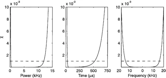
is the end result of the optimization algorithm; a set of piecewise constant time dependent parameters that gives a 1800 rotation on Alanine's first spin. 26 3-3 The three penalty functions for the pulse power, time and frequency.

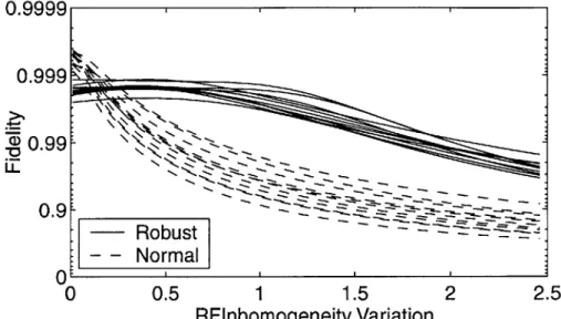
Nega-tive powers, powers greater than 12kHz, and frequencies greater than 16kHz are strongly penalized. Transient errors are lessened by penalizing durations shorter than 30ps. Otherwise, preference is given to shorter duration pulses. 27 3-4 The fidelity performance as logarithmic distance to unity is shown for 11

ro-bust and 11 uncompensated pulses as the width of RF power density function is scaled by a constant factor. The robust pulses show a greater ability to maintain fidelity as greater RF inhomogeneity is introduced . . . . . 29

4-1 A feedback method of realizing the desired robust pulse. The desired pulse requires a set of step functions. The uncorrected waveform shows transient and steady state errors. The corrected waveform more closely tracks the desired waveform . . . . 32 4-2 On the left is a an initial guess of the optimization parameters. On the right

is the end result of the optimization algorithm; a set of piecewise constant time dependent parameters that gives a 180' rotation on Alanine's first spin. 33 4-3 A Summary of Pulse Performance. On the left is pulses found without RF

inhomogeneity compensation. On the right is pulses found with RF inhomo-geneity com pensation. . . . . 35 5-1 The fidelity performance of 11 robust and 11 uncompensated pulses as their

RF power is scaled by a constant factor. The robust pulses show a greater ability to maintain fidelity especially at attenuated RF powers. . . . . 37 5-2 Maximum Fidelities found as function of Maximum Power.High fidelity pulses

were found in high power regime defined by the minimum chemical shift difference. . . . . 38

Chapter 1

Introduction

1.1

Background on QIP

Feynman, in 1982, proposed the idea of using dynamical systems governed by quantum mechanics to simulate quantum physics [1]. Quantum mechanical simulation is difficult on a classical computer. An N particle system's state requires a vector of 2N elements, so

for large N, just writing the wave function, let alone simulating its dynamics, is infeasi-ble. A quantum information processor can act as an analog simulation of other quantum mechanical systems resources [4]. It can do this by mapping the simulated system's state to that of the quantum information processor and using a set of universal gates to enact the simulated dynamics. Additionally, Feynman's idea has been expanded to the use of quantum mechanical systems to do computations. This new field of Quantum Information Processing (QIP) has led to quantum mechanical search and factoring algorithms that give exponential speed improvements over their classical counterparts [2], [3]. (These algorithms would revolutionize the current field of encryption.)

The advantages of QIP arise from the ability of a quantum mechanical particle to be in a superposition of states. In classical computation, a bit is either 10) or 11); on or off. A qubit 10) can be in an arbitrary superposition of these two classical states;

I)

1.2

NMR as a paradigm for QIP

Recently, advances in QIP have included experiments. Quantum control has been demon-strated in quantum optics [5], [6] and nuclear magnetic resonance (NMR) [7], [8], [9]. Warren

provides a summary of their advances [10]. NMR has been used to experimentally demon-strate quantum error correction [11], [12], quantum simulation [13], and quantum algorithms

[14], [15] such as the quantum Fourier transform [16].

The NMR paradigm for QIP currently uses a solution of molecules dissolved in a liquid solvent. Usually the molecule will contain atomic nuclei that are spin 1/2 particles such

as H1 and C13. Each of these spin 1/2 particles provide one qubit in the QIP. Although there are approximately Avagadro's number of molecules in the solution, the system does not have that many qubits. This is because solution dynamics remove the intermolecular dipolar coupling. (This leaves each of the molecules to be indifferentiable from the other.) As a result, the quantum information processing is carried out on an ensemble of molecules whose spin dynamics closely parallel the spin dynamics of an individual molecule. At room temperature, the state of the ensemble is highly mixed. The small imbalance between the spin up and spin down populations is on the order of 10-6 and provides the NMR signal

[17].

1.3

Experimental Apparatus

The NMR spectrometer is composed of a static magnetic field, a probe, radio frequency transmitter. The probe includes an inductor coil that applies time varying magnetic fields to the sample. The direction of the static magnetic field is conventionally taken to be in the z direction. For QIP, its strength is usually on the order of 10 Tesla. Figure 1-1 shows a 9.6MHz magnet. Much like classical tops in the earth's gravitational field, this static magnetic field aligns nuclei with spin upwards or downwards. An alternating current, usually in the radio frequency range, is run through the inductor coil, and a time varying magnetic field of the same frequency is applied to the sample within. The addition of this secondary field allows for control of the spin system's orientation state.

The RF coil is also responsible for signal detection. Figure 1-2 shows a schematic diagram of the RF coil's dual function. In its first function, the gate is closed. A RF frequency current is amplified and then delivered to the sample as a magnetic field. In its

Z

radient Coil

RF

Coil

G

B

Liquid State Sample

in a Test Tube

Figure 1-1: On the left is a photo of a 9.6T magnet. On the right, is a diagram of the RF coil that applies time varying magnetic fields to the sample within.

second state, when the spin system is not being excited, the gate is open. The spin system evolves freely, causes a time varying magnetic field which is detected as an alternating current in the coil. Because the current's frequency is on the order 400 megaHertz, it is convenient to mix the signal down to an audio signal.

1.4

Motivation for Robust Control

NMR provides a test-bed for investigating QIP experiments. Pulses can be applied experi-mentally to manipulate a spin system such that its final state is equivalent to the output of a chosen theoretical algorithm. One challenge in QIP is that the errors in the implementation of these pulses often cause a loss of information during the course of the algorithm. One type of error, called incoherent errors, occurs when the different parts of an ensemble have experimentally different evolutions. In NMR, this type of error is exemplified by

Frequency Source

RF Coil

Static

Field

MAxermp

Pre-Amp

Figure 1-2: A schematic diagram of the RF coil's dual function; external control of the spin system and signal detection [18].

magnetic field strength varies spatially. The signal from the ensemble is a collection of evolutions based upon a distribution of the RF coil's magnetic field strengths.

Because these errors cause an exponential loss of information, it is critical that they be reduced. The proposed method is to develop a set of pulses that are insensitive towards variations in the pulse power. If a particular evolution does not require a high accuracy in the RF pulse power, then such evolution would be more capable of retaining information in the presence of RF inhomogeneities.

1.5

Overview of Approach

The approach to finding a set of robust control pulses that give desired evolutions is straight-forward. Chapter 2 will acquaint the reader with detailed dynamics of a liquid state NMR system. Once the reader has gained knowledge of the system Hamiltonian, Chapter 3 will step back and define a metric for the experimental precision of an RF Pulse with respect to a desired theoretical evolution. It will continue by casting a direct relationship between RF inhomogeneity and this metric. Next, it will show a method of measuring the degree of RF inhomogeneity and use this information in the development of a compensation algorithm that yields robust control. Chapter 4 will discuss the experimental issues of realizing these robust pulses and then summarize their experimental performance relative to a non-robust

method. Finally, Chapter 5 will discuss various aspects of this robust control method, explore its achievable limits and propose extensions of the method to other fields of control.

Chapter 2

Dynamics of Liquid State Nuclear

Magnetic Resonance

The static magnetic field of the NMR apparatus aligns spin 1/2 particles into one of two eigenstates: the ground or up state and the excited or down state. This chapter will explain this physics, show how the spin states can be used as qubits and show how the spin system can be excited using time varying radio frequency magnetic field pulses.

2.1

Spin Wavefunctions, Operators, and Bra-Kets

A spin 1/2 particle is measured as having one of two discrete values of spin ±h/2 [19]. These two values can be mapped on to the standard basis vectors.

1 ₀₍₂₁

10)= ) (2 )

01

where the ket notation of 10) and 11) refers to the positive and negative value of the z component of the spin respectively. A general spin state b is a superposition of these values[19],

I) = c+10) + cI1) = c+ (2.2)

C-where c2 + c2 = 1. The dynamics of the spin state is given by the time independent Schrddinger's Equation,

-

(I

-I

(t))

(2.3)

dt h

where R is the system Hamiltonian. For a time independent Hamiltonian, the evolution of the spin state is described by a unitary operation.

10(-))

It is convenient to introduce the Pauli spin operators o-, a-y and a-, and the identity operator as a basis of the Hamiltonian space.

0 1 0 z1 0

~x=

[

Y

]

r=[

(2.5)

1 0 -z0 0 -1

These operators are hermitian and have many useful mathematically and physically signif-icant properties[19],

= 2, ao =

a, det(-i)

-1,

Tr(a)

0

(2.6)

Additionally, they obey the anti-commutation relation {o-i, o-a

}

relation [a, o-y] = 2ia-, which also holds for all cyclical permutations of the operators.

Anti-cyclical permutations give a minus sign. These operators have the physical significance that they give the expectation value of the spin wave function (a) with respect to the chosen cartesian axis[19].

(o-x)

= (4'XIaO)

(-y)

=

(Mao-yIlo)

(o-z) = (O|azl)

(2.7)

(x) is the expectation value of an arbitrary operator x. The bra notation (xI is the complex conjugate transpose of the ket notation

Ix),

Ix)(xl

2.2

A Spin 1/2 Particle in the Static Magnetic Field

In a magnetic field B, the energy of a spin is similar to that of a classical magnetic moment Iy. It will align or anti-align with the field and have an energy of [20],

E =-y B (2.8)

Similarly, a spin 1/2 particle's magnetic moment is given by[21],

p = yhm (2.9)

where -y is the gyromagnetic ratio, and m is the value of the spin. For a static field B = Bo , the matrix representation of the Hamiltonian (often referred to as the Zeeman Hamiltonian)

is[21],

~yhB

2 "oz(2.10)

2

2.3

Thermal Excitation and the Density Matrix

A typical liquid state NMR sample, placed in a test tube, will have many spin 1/2 parti-cles. Spins are thermally excited away from the ground state according to the Boltzmann distribution,

Ne 2

KbT 1 ±yhBo

WLN m-yBo 2 4KbT (2.11)

so that a fraction w+ are in the ground state and w- are in the excited state[17]. This mixed ensemble can not be represented with a single wave function, and requires the introduction of the density matrix p[19],

p =

Zwilvi

i

whose evolution is given by the Liouville-Von Neumann equation;

For a time independent Hamiltonian, the evolution of the density matrix is given by a unitary transformation.

p(r) = e-' p()e*Hi (2.14)

Additionally, the concept of an expectation value is replaced by the ensemble average[19],

[X] = >jwi < 4'j xjb >= Tr(pX) (2.15)

2.4

The External Hamiltonian and the Rotating Frame

In addition to the BO static field, the NMR spectrometer uses an inductor coil to create small magnetic fields oriented along an axis orthogonal to

2.

H =z + B, X (2.16)

2 Bo

For B1

<

-yBouz (-f t+b)z ) %(wf t±S)aTz )

2

= B _ B 2 (2.17)

where the second term is defined as the external Hamiltonian Hext. A different picture

emerges when the dynamics are described in a frame rotating at the frequency of the applied magnetic field wrf. The rotating frame density matrix p and Hamiltonian ' are found by applying a unitary frame change operator U,

Ur = e2'rfT z (2.18)

Plugging these quantities into the Liouville-Von Neumann equation yields a time indepen-dent effective Hamiltonian H of

~ Wrf _{W f-} -z (Wo _(WO - Wrf) _{-zf) -} W1 _oU

(2.20)

2 2 2

where the Larmor Frequency and the RF power are defined as wo = -7Bo and wi = -- B1

respectively. One should note the resonance condition wo = Wrf entirely eliminates the u-z term in the effective Hamiltonian. The time independence of the rotating frame effective Hamiltonian allows for solution of the output density matrix by Equation 2.14.

2.5

Multiple Qubit Molecules and the Spin-Spin Scalar J

coupling

So far, the density matrix and system Hamiltonian has been described for single spin molecules. However, for the purposes of QIP, it is necessary to investigate multi-spin molecules like C-13 labelled Alanine. Figure 2-1 shows a graphical model of the molecule. Here, the three C-13 labelled nuclei are spin 1/2 particles that act as qubits. For a pure

iN

''

1-2286.5

_35.0

_C2

0

7167.8 54.1

-1.3

C

C1

C2

C3I

Figure 2-1: A Graphical Representation of the Alanine Molecule. At the bottom right, the chemical shift frequencies and the scalar coupling strengths are shown in units of Hz.

rep-resented by a 2N x 2N density matrix. This expanded space is spanned by N Kroenicker

products of any of the Pauli spin operators and identity.

Each carbon nuclei acts as a magnetic dipole, and hence the Hamiltonian includes a Zeeman term for each qubit. Each carbon nuclei has the same gyromagnetic ratio, but its surrounding electron clouds shields the nucleus from the static field to different degrees. As a result, each carbon nuclei will experience a unique local magnetic field. In the rotating frame, the sum of the Zeeman terms gives the chemical shift Hamiltonian,

N

7Ycs = ( oi - rf) Uzi (2.21)

where the subscript i denotes the spin index. Figure 2-1 shows the chemical shift frequencies of Alanine's three spins. Additionally, the azi notation implies two Kroenicker products with identity 12, 13, on the second and third spins. The introduction of multiple spin 1/2 particles to a molecule also brings about a spin-spin scalar coupling that acts through electrons of the molecular bonds. Any two spins i and

j

H = " E

i

The scalar coupling Hamiltonian is usually simplified using weak coupling limit. When the difference in chemical shift frequencies of any two spins woi - woj is much greater than their

scalar coupling constant Jij, the ui - u-2j and uyi , Uy become nonsecular. In other words, the ozi -O-zj term, because it commutes with the Zeeman Hamiltonian, will have a greater effect on the eigenvalues of the total Hamiltonian [17]. The internal Hamiltonian Hint is then defined as the sum of the chemical shift and weak scalar coupling Hamiltonians.

N

Hint =

I

j

k=1 k

With the Zeeman, scalar coupling, and external Hamiltonians defined, the output den-sity matrix in the rotating frame can be found by Equation 2.14. Transforming back into the lab frame requires the inverse frame change operator, U;-1 ₌

and gives the output density matrix in the lab frame,

p(T) = U71e-*i pine*k*Ur (2.24)

This yields the overall unitary evolution operator Unet.

Unet = U-le-zir (2.25)

Once the internal and external Hamiltonians have been well defined, steps can be taken to manipulate their dynamics such that the spin system follows a desired evolution.

Chapter 3

A Method for Compensating for

Incoherent Errors

The previous chapter developed the Hamiltonian of a liquid state NMR system, and showed its dependence on the chemical shifts, spin scalar coupling, and the RF power. This chapter will continue by explaining coherent and incoherent errors in quantum control; especially those that arise when this Hamiltonian is experimentally implemented. It will briefly review previous methods of compensation and then will proceed to describe a new general method provided that one has an understanding of the system's dynamics and its incoherent errors.

3.1

Incoherent Errors in Quantum Control

Quantum Information Processing uses a sequence of unitary operations to map a set of input states to a set of output states. Such a quantum algorithm requires a set of universal gates which comprise its building blocks. The physical implementation of an arbitrary algorithm requires a quantum system with a Hamiltonian that has a sufficient number of control parameters such that it allows for the generation of the universal set of gates [22].

Various types of errors occur in the physical implementation of a quantum gate. Given an arbitrary input density matrix pin, a quantum gate will map it ideally to a theoretical output density matrix Pth. Assuming that the transformation is a unitary operation Uth,

In the physical implementation, the input density matrix is mapped instead to pout through the unitary operator Unet. The projection P of Pout onto Pth provides a good metric of the similarity of the two density matrices[24].

P = Tr(p0utPth) (3.2)

uTr(ptpeh)

While a measure of the accuracy of the output density matrix is useful, it does not predict its accuracy with respect to a theoretical density matrix for a different input state. Instead, a metric called the gate fidelity, F, is needed. For an N spin system, the fidelity is defined as the average of all of the projections, Pk, for an orthogonal basis of inputs Pk,

22N

F = 221 Pk (3.3)

k

Fortunato et al. show that this is equivalent to a direct comparison of the ideal theoretical unitary operator and the experimental unitary operator[9].

1t 2(34

F Tr (Uh net)

₍₎

22N

One should note that the fidelity approaches unity as Uth and Unet become the same. While perfect control, or a fidelity of one is not required, fault tolerance requires a fidelity of at least 0.9999 to 0.999999 depending on the assumptions used[23].

Coherent errors as well as incoherent errors lower the gate fidelity. Coherent errors arise due to the dissimilarity of two unitary operators. Nevertheless, the physical system as an ensemble, still evolves due to a single net unitary operator. Incoherent errors arise when portions of the ensemble evolve due to separate Krauss operators, Ak. The output density matrix is then given by,

Pout =

5

k and the gate fidelity becomes[9],

F 1 (36

F 22N I Tr(UhA )1 (3.6)

k

pri-marily addresses spatial incoherence errors, Section 5.2 will propose extensions to temporal incoherence. A good example of spatial incoherence in liquid state NMR is the RF inho-mogeneity. Ideally, the coil will produce a spatially uniform magnetic field with a constant amplitude. In actuality, the RF magnetic field will vary in amplitude across the volume of the sample. The RF field power amplitudes akw1, weighted by fractions of the volume bk gives the evolution of the input density matrix.

Pout = bkU pinUt (3.7)

k

where the Unitary operator Uk is dependent on the RF amplitude;

Uk = U;-le--(Hint+Z 2- (3.8)

One should note that Equation 3.7 follows the form of Equation 3.5 when Ak = v/I-Uk. Hence, it will cause incoherent errors with respect to a theoretical unitary gate

Uth-The degree of these incoherent errors can be described analytically for a single spin system. For an on-resonance pulse (wo = w.f), the internal Hamiltonian vanishes, and an

ideal coil is only capable of producing transformations of the form:

Uth = e -%W1ze TeO02 (3.9)

A non-ideal coil will have Krauss operators of the form,

Ak = 1e-Oa e 2l e* (3.10)

Substituting Equations 3.9 and 3.10 into Equation 3.4 directly yields the fidelity as function of the RF inhomogeneity description.

F = E bk cos2 [(1 - ack)WiT] (3.11)

k

Using the above result, a uniform distribution with a width of 10 percent immediately causes the fidelity to drop to 0.99875. This drop is very significant when compared to the fault tolerance threshold. Additionally, one can expect that the error due to RF inhomogeneity

3.2

A Brief Review of Compensation for RF Inhomogeneity

Previous methods in compensating for RF Inhomogeneity have typically used a sequence of pulses that have certain symmetries that to first order average out RF inhomogeneity errors while still achieving the desired control on the spin system. Such ideas are prevalent in a variety of well developed 'echo' methods [25], [26], [27]. Shaka et al proposed a method based upon 90' and 270o rotations placed sequentially in super-cycles [28]. Finally, an extensive review of composite pulse methods is provided by Levitt [29].

3.3

An Method for Compensation

From Equation 3.6, the compensation problem is defined as finding a set of Krauss operators that give a fidelity that approaches unity for a given theoretical gate Uth. Each of the Krauss operators will differ from the others by their dependence on the power density function. Each will also depend on a set of parameters whose values are the same for all of the Krauss operators. In the proposed method, ak and bk differentiate the Krauss operators while the four parameters wi, wrf, <, and T, are constant for each operator. These parameters are chosen for their physical significance in the experimental implementation. No statement is made about whether this is the only or best parameterization. With it, however, the problem reduces to finding optimal values of RF power, frequency, phase and time given a measured set of values ak and bk. Prior to starting a robust compensation algorithm, it is necessary to measure the power density function that describe these values.

3.3.1 Experimental Determination of RF Inhomogeneity

The RF inhomogeneity can be determined by measuring the nutation frequency of the NMR signal after a single pulse of variable duration. A molecule with a single carbon-13 labelled spin, Chloroform (CHCl3 was chosen as the sample. A single on resonance pulse 0 = wiT

about the x-axis was applied and signal was measured. The RF power was chosen such that its amplitude is much greater than any scalar coupling constants. The pulse was varied in duration and then repeated. Considering only the carbon species, the output density

matrix for the 1th pulse is,

P1 = U -E( cos(wkTI) + ',

S

k k

and the free induction decay signal is given by

b 2

S(l, t) = sin(Wkri e-tlT2 (3.13)

k

An extra factor of of bk is acquired because the RF coil is also used as the receiver and has the same sensitivity to detecting magnetic fields as delivering them. In order to maximize signal to noise, the signal is integrated in time. The Fourier transform with respect wi is then taken;

S(w) = Tij b2 [6(w - W1k) - 6(w - W1)1 (3.14)

k

This signal describes the density bk of a given power wlk. This experiment was performed on a Bruker 300 MHz, as well as a 400 MHz spectrometer. Figure 3-1 shows the experimental results in dimensionless units and normalized to integrate to unity. The RF coil in the 300MHz magnet had a density function width of 6.23 percent at its half maximum. The average power delivered to the sample by this coil was attenuated from the ideal value by 3.50 percent. The 400 MHz magnet had a similar result. Its width and attenuation were 7.00 and 5.64 percent respectively. The RF coils in both magnets also show an asymmetry in the density of powers delivered to the sample. As expected, both show long tails below the ideal power of wi. However, a significant portion of the sample is exposed to powers greater than wi. This experimental data was then fit with a polynomial regression for powers below the reference and fit with an exponential regression for higher powers. This fit directly gives the power levels akwl and their respective fractions bk, required for the optimization algorithm.

3.3.2 Optimization Algorithm

Once the various power levels and their weighting is found, optimal values of w1, Wrf,

#

T can be found using numerical methods. First, a physically implementable initial guess

RF

Inhomogeneity on a 300 MHz Spectrometer

RF

Inhomogeneity a 400 MHz Spectrometer

Normalized Power (unitless)

Figure 3-1: On the 300MHz spectrometer, the width of the density function at half the maximum value was 6.23 percent. Similarly, the 400 MHz spectrometer had a width of 7.00 percent. Integrating over the density functions yields an average delivered power attenuated by 3.50 and 5.64 percent respectively.

No guarantee can be made that the algorithm will find the global optima. Instead, different guesses can converge to different optima with nearly equivalent fidelities. Next, the set of Krauss operators associated with these pulses are calculated, the pulse fidelity with respect to a given gate is calculated. A new quantity, x defined as x = 1-F, is then minimized using

a Nelder-Mead simplex search. If the optimal parameters do not meet a chosen convergence criterion i.e. x = 0.001, the pulse duration T is broken into two separate durations Ti and

-2. Each of these durations will have a power, frequency, phase and duration such that the new search has a total of eight parameters to be optimized. In effect, the algorithm is expanded to find two separate sets of Krauss operators. Equivalently, the RF pulse power, frequency, phase and time become piecewise constant functions in time. This process of adding a new duration with four new parameters is repeated as many times as necessary. Equation 3.7 still determines the output density matrix, and the M sets of Krauss operators

can be combined to create a single set of effective Krauss operators.

M

Ak = \/k rUkm (3.15)

m

where Ukm is defined by Equation 3.8 and wi, wf, q and r are dependent on the duration index m. Figure 3-2 shows how an initial guess of constant RF pulse parameters becomes a set of piecewise constant time dependent parameters developed for a 1800 rotation on Alanine's first spin.

) 100 200 300 400 ) 100 200 300 400 15 10 (D 5 0 a. 0 10 N 5 0 -5 L- -10 360 270 SO180 90 0' 300 400 15 10 (D 5 0 01 0 50 100 150 200 250 10 N 5 0 U- -10, 0 50 100 150 200 250 - 360 ( 270 C 90 0 0 50 100 150 200 250 Time (gs)

Figure 3-2: On the left is a an initial guess of the optimization parameters. On the right is the end result of the optimization algorithm; a set of piecewise constant time dependent parameters that gives a 1800 rotation on Alanine's first spin.

In the minimization routine, the optimal parameters must remain within a physically implementable search space defined previously in the creation of the initial guess. To ensure a feasible solution, the search is constrained by adding to the chi function functions that penalize non-feasible value of the parameters. Specifically,

100 200 Time (ps)

-.

0

where Xwj, X wf and X, are penalty functions that depend on each of the parameters respectively. These functions are nearly flat in the feasible region and are sharply increasing at the regions' boundaries. Many types of smooth functions can be used while still retaining convergence. Figure 3-3 shows the shape of the functions used in this study. The power

x 10-3 0 5 10 15 Power (kHz) x 10-3 10 - . 8- 6-4 2-0 250 500 750 Time (gs) X 10-3 10 x .o. 8 6 4 2 20 10 0 10 20 Frequency (kHz)

Figure 3-3: The three penalty functions for the pulse power, time and frequency. Negative powers, powers greater than 12kHz, and frequencies greater than 16kHz are strongly penal-ized. Transient errors are lessened by penalizing durations shorter than 30[ps. Otherwise, preference is given to shorter duration pulses.

penalty function used is,

XW1 = e(-2.3026xj0-3min(wi(t))) + (3.1623 * 10-10) e(2.3026*-10-4 max(wi(t))) (3.17)

An exponentially increasing penalty prevents negative powers for the duration of the pulse. Similarly, the second prevents high powers that are capable of "arching" or "heating" the coil. The time penalty function is,

X- = 10e(-2.3026105min(Tr)) + (1.2916 * 10-5) e(+1.2792*104T) (3.18)

The first term prevents any set of parameters from being applied for too short of a time period. In this case, periods shorter than 30ps will have errors dominated by transients in the experimental implementation. The second term in the penalty function is a less steep exponential. Here the function has two purposes. It eliminates pulses longer than 500ps,

10

8

6

4

and gives preference to pulses of shorter total duration. Long pulses, especially when used in sequences) are prone to decoherent errors such as relaxation [17]. Lastly, the frequency penalty function is,

Xrf = 10-6e(9.161710- 51max(wrf (t))I) (3.19)

Here negative frequencies are allowed, but more importantly the magnitude of the frequency is limited to 16. The RF frequency must remain within the bandwidth capabilities of the spectrometer.

3.4

Summary of Pulse Parameters

The above algorithm was used to make a set of 11 robust pulses that each implement a given theoretical unitary gate. Also, the same algorithm was used to make 'normal' pulses; i.e. pulses that did not compensate for incoherent errors in the calculation of the fidelity. The parameters for robust pulses can be found in Appendix B while uncompensated pulse parameters can be found in C. The uncompensated pulses had an average duration of 236.49 ps. This time was usually broken into four shorter durations; while some pulses had as few as three constant durations and as many as seven durations. These pulses on average had a maximum power of 8.7255 kHz; while highest power pulses had a power of 10.77kHz. The compensated pulses were on significantly longer; lasting on average 341.99

ps. This is, however, much shorter than conventional methods of creating single spin

rotations. Qualitatively, the biggest difference in the two sets of pulses. The robust pulses as a set required on average seven constant durations with a minimum of six durations and a maximum of 12. The maximum power numbers were also higher, but not as significantly. On average, the maximum power was 10.70kHz, and the most powerful pulse required

11.3kHz.

3.5

Simulated Robustness to RF Inhomogeneity

The robustness of the two sets of the pulses can also be directly compared in simulation. Here robustness is defined as the ability for a particular pulse to maintain fidelity as sys-tematic errors are introduced. For this simulation of robustness, the width of the RF power

was calculated. Figure 3-4 shows the performance of the two sets of eleven pulses. For the

0.9999

0.999

)0.99

0.9

Robust

Normal

0

:

I

0

0.5

1

1.5

2

2.5

RFinhomogeneity

Variation

Figure 3-4: The fidelity performance as logarithmic distance to unity is shown for 11 robust and 11 uncompensated pulses as the width of RF power density function is scaled by a constant factor. The robust pulses show a greater ability to maintain fidelity as greater RF inhomogeneity is introduced.

experimentally measured inhomogeneity, the robust pulses out perform the uncompensated pulses by an order of magnitude. Additionally, they have a nearly constant fidelity for more ideal RF coils. The uncompensated pulses, however, show a steep degradation as RF inhomogeneity is introduced, and only show high performance for nearly ideal coils. At RF inhomogeneities greater than the ones experimentally measured, the uncompensated pulses degrade at a slower, but still nearly exponential rate. This rate is approximately the same for both sets of pulses for very large RF inhomogeneities. It is not clear why the robust pulses's performance begins to degrade significantly after the introduction of RF inhomo-geneity strengths greater than the one experimentally measured. Two possible explanations exist. The algorithm can be compensating fully for the errors used as its input. In which case, finding new pulses for an RF coil with a different power density function will show a break point in the performance at that power density function's width. On the other hand, the performance break point can be a function of the internal dynamics of the molecule. In that case, the performance break point will be fixed at the current width of approxi-mately 6.23 percent. It is likely that both explanations contribute, and this question can be investigated further by making pulses for a variety of different RF inhomogeneity strengths.

These simulated results suggest that the proposed algorithm is capable of finding a set of parameters such that the density matrix's evolution will closely correspond to the desired unitary gate. Additionally, they show that the robust pulses will out perform the uncompensated pulses when they are experimentally implemented and are in the presence of incoherent evolutions.

Chapter 4

Experimental Results

Chapter 3 described the coherent and incoherent errors that arise when experimentally implementing theoretical unitary gates. It went on to provide an algorithm that finds a set of pulse parameters such that the evolution in experiment has minimal coherent errors and is robust towards incoherent errors. This chapter will discuss how these parameters can be realized experimentally. It will then measure the performance of experimental gates with respect to the theoretical ones.

4.1

Experimental Realization of Waveform

Figure 3-2 shows that a given pulse is defined by a set of piecewise time dependent param-eters. The difficulty with this is that these functions are not differentiable throughout their whole duration; specifically at the boundaries of any two durations. Real physical systems such as inductor coils follow ordinary diffential equations are not capable of instantaneous changes in their time response. Because the gate fidelity is tuned to these pulse parameters, any experimental derivation from them will introduce experimental errors.

In order to eliminate errors due to waveform distortion, a feedback method was used. (Throughout, this thesis the RF coil has been referred to as a single entity. In actuality, there are two coils; one to excite hydrogen nuclei and the other to excite carbon nuclei.) The robust pulses were digitized and then run on the carbon channel. Meanwhile a digital measurement of the applied magnetic field was made using the Hydrogen coil. The difference between the measured pulse and the desired pulse was then used to create a corrected digital waveform. This feedback process was iterated between four and six times such that the new

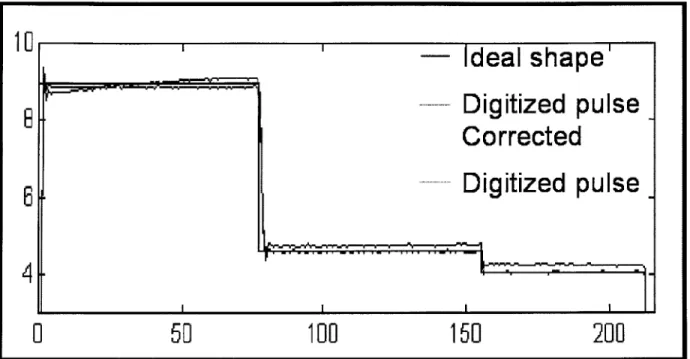
corrected waveform closely matched the desired pulse found by the algorithm. Figure 4-1 shows a comparison of the desired, uncorrected and corrected waveforms further details of this method can be found at [30]

-

Ideal shape'

Digitized pulse

Corrected

---

D

ig itiz

e d p u

lse

41

0

50

100

150

200

Figure 4-1: A feedback method of realizing the desired robust pulse. The desired pulse requires a set of step functions. The uncorrected waveform shows transient and steady state errors. The corrected waveform more closely tracks the desired waveform.

4.2

State and Process Tomography

Once the preparation steps have been taken to implement the pulse parameters, the ex-periment can be performed. However, as will all quantum mechanical systems special care must be taken to make the proper measurements. The goals is to extract the experimental fidelity for a given set of pulse parameters. This requires a method called Quantum Pro-cess Tomography (QPT) [31]. By Equation 3.3, 22N states needed to be prepared for each

experiment to be done. This is difficult, but is further complicated by the fact that the output density matrix can not be acquired in a single measurement. In NMR only single quantum coherence product operators are observable [17]. In other words, the NMR signal

three spin system like Alanine, the 24 observables are,

Jxl Uxlz2 UxIz3 Ux1Uz2Oz3 Uyl Uylz2 JylOz3 Uy1Uz2Uz3

Ex2 UzlOx2 Ux2Uz3 Uzlx2Uz3 Uy2 Ozly2 %y2Uz3 Uz1'y2Oz3 (4.1)

U3 (zlx3 Uz2Ux3 Uzlz2Ux3 Uy3 UzlUy3 Uz2Uy3 az1'z2Uy3

In order to obtain the coefficients of the product operators, QPT requires another method called quantum state tomography [31]. This process is done by applying 'read out' pulses that rotate non-observable product operators to observables. Figure 4-2 gives a conceptual diagram of the entire process of QPT. An infinite number of different sets of read out pulses

State Preparation Robust Read Out

P u lse P u lse * * J P u lse Pobserva 'l

Figure 4-2: On the left is a an initial guess of the optimization parameters. On the right is the end result of the optimization algorithm; a set of piecewise constant time dependent parameters that gives a 1800 rotation on Alanine's first spin.

yield all the product operators, but the following set of 8 E pulses is sufficient.

r1 r 1,2 7 12,3 3 7 1,2,3 11,2,3

(4.2)

where the short hand 7rI means the unitary operation of ' rotation on the first spin around

the x axis.

Once all of the product operators have been shown to be experimentally accessible, it is necessary to determine their weighting from the NMR signal. Neglecting noise, the NMR signal for Alanine has 12 sinusoidal components with distinct frequencies; one for each spin and its positive and negative coupling to the remaining two spins. More specifically, these frequencies Wijk are found from the internal Hamiltonian [17].

Wijk 1Woi ± rij ± irJik

(4.3)

where i,j,k are different permutations of the vector [1 2 3]. The signal will also have phase information stored within its real and imaginary parts. Finally, the NMR signal has an

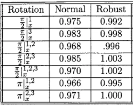
Rotation Normal Robust 0.975 0.992 0.983 0.998 7 11,2 0.968 .996

E3

0.970

1.002

Table 4.1: Correlations of seven pulses; robust and uncompensated. All of the robust pulses show an improved fidelity over uncompensated pulses. All values have an error margin of ±0.01.

exponential relaxation with time constant T2. The signal's general form is;

S(t) = e(-t/T2)

( (

+

(4.4)

i j k

The signal's spectra can be obtained by taking its Fourier transform. The result is a sum of 12 Lorentzians each described by two parameters; the magnitude of its real and imaginary parts. These 24 parameters map linearly to the coefficients of the 24 observables. For example, the coefficient to u.i is the average of the magnitudes of the four Lorentzians with highest frequency.

4.3

Experimental Results

Two sets of seven pulses were made. The first did not compensate for RF inhomogeneity while the second did. Quantum Process Tomography was done on each of the fourteen pulses. To cut down on experiment time, only three of the 64 input states. These states are Ej a-2j, Ej oyi, and E> u-zi. The resulting correlations were calculated and are presented in 4.3. All of the robust pulses yielded correlations greater than their uncompensated counterparts. The average improvement in the correlation is 0.024. This is well beyond the estimated error margin of +0.01.

4.4

Degree of Improvement in RF Inhomogeneity

Compen-sation

As stated in the previous section, the experimental fidelity was improved by using pulses robust towards RF inhomogeneity. Figure 4-3 summarizes the estimated error contributions of all the pulses. Of the five major error types, coherent errors, pulse distortions,

measure-0.05

0.04 k

0.03[

0.02 F

0.01

k

0 L_

0.0007

Figure 4-3: A Summary of Pulse Performance. On the left is pulses found without RF inhomogeneity compensation. On the right is pulses found with RF inhomogeneity com-pensation.

ment errors, decoherence, and RF inhomogeneity, the last was the greatest in magnitude. After compensation, it was reduced by approximately a factor of six. This is about the same as the magnitude of measurement errors. The combination of these two method reduced errors by approximately 60 percent.

0.05

0.04 k

0.03 F

0.02 k

0.01 k

0 L_

-

-Chapter 5

Discussion

Chatpers 3 and 4 showed the theoretical and experimental performance of pulses that im-plement evolutions that are robust towards incoherent errors. Theoretically, they show well maintained fidelities in the presence of RF inhomogeneity, and experimentally high correla-tion values were measured. This chapter will continue by showing further aspects of these robust pulses, and it will try to propose extensions to other problems while illuminating the method's limitations.

5.1

Further Aspects of Pulse Performance

Chapter 3 showed previously in Figure 3-4 that the algorithm yields a set of robust pulse parameters. Specifically, performance is maintained as the RF inhomogeneity strength is varied. This, however, does not predict the performance of the pulse parameters when RF coil is perfectly homogeneous but has systematic bias in its power. Figure 5-1 shows the fidelity of the pulse as its power is amplified by a constant factor.

As expected the uncompensated pulses show a sensitivity to the scaling of the RF pulse power. Comparatively, the robust pulses maintain their fidelity especially for attenuations of the pulse power. Interestingly, the robust pulses on average perform best with a constant attenuation of about 3 percent. This is close to the average power of 3.50 percent attenuation delivered by the RF coil. Finally, this asymmetry of the robust pulses, in comparison to the symmetry of the compensated ones, suggests that it is due to asymmetry of the RF coil's power density function. In fact, this result correlates to the power density function's

n

--

Robust

0.99 -

-

Normal

0.9

0.85

0.9

0.95

1

1.05

1.1

1.15

RF Scaling

Figure 5-1: The fidelity performance of 11 robust and 11 uncompensated pulses as their RF power is scaled by a constant factor. The robust pulses show a greater ability to maintain fidelity especially at attenuated RF powers.

reasonable to conjecture that this algorithm would yield the opposite asymmetry if given a power density function with an excess of higher powers.

5.2

Pulse Fidelity in the Presence of Temporally Incoherent

Errors

The above figure also suggests a robustness towards some time types of temporally inco-herent errors. One can imagine an experimental situation where many pulses are cascaded and the pulse power varies but at a rate significantly slower than the duration of the pulse. In this instance, each pulse individually will create an evolution robust to the variation in the pulse power; and the train of pulses as a whole will more closely approximate the desired evolution than a train of pulses that did not compensate for incoherent errors. This argument is of great importance because QIP requires the use cascaded unitary operations that implement a series of one and two qubit quantum gates.

5.3

Exploring Achievable Fidelities

The proposed algorithm shows a good way of finding optimal RF pulse parameters in the presence of incoherent errors. Additionally, it can be repeatedly used to understand the depth and frequency of optimal points in the search space. Specifically, pulses can be found as the search constraints are relaxed and tightened; thereby simulating this method's achievable limits of control using a variety of equipment. A perfectly homogenous coil was assumed and the a set of parameter guesses was made using all of the previously mentioned intervals. While varying the second term in the power penalty function, these guesses were used to find pulses that implement a 90 degree rotation on Alanine's second carbon spin. Effectively, the upper limit on allowed powers was varied. Figure 5-2 shows the maximum fidelities of these pulses as a function of their maximum power. A total of 2088, 1222, and

Maximum Fidelity Found for a Three Spin n/2]2 Pulse

0.9999

0.999

0.99

0.9

100 10 1 M10 P 10 3

Maximum Pulse Power (Hz)

Figure 5-2: Maximum Fidelities found as function of Maximum Power.High fidelity pulses were found in high power regime defined by the minimum chemical shift difference.

599 pulses were made for 300, 600, and 800 MHz magnets respectively. While this method does not ensure finding globally optimal fidelities, the maximal fidelity among many local

-0 z0 MH - - .-U -A50M;zl. -z --4- 300 MH .- A 500 MH E - 800 MH --- a --- im . . .I I . . I . n 10

analytical result. The dotted vertical lines show the minimum chemical shift difference for alanine on 300, 600 and 800 MHz magnets. The achievable fidelities drop dramatically in a low power regime defined by alanine's minimum chemical difference. For this molecule's high power regime, this algorithm is theoretically capable of achieving fidelities of at least 0.999. It appears that increasingly better fidelities can be achieved when a number of durations with increasingly loose power restrictions are used. Finally, significantly better fidelities were found for higher fields. As the static magnetic field strength is increased, the chemical shift differences increase with respect to the constant scalar coupling leading to a greater ability to make selective rotations. For an 800 MHz magnet, theoretical fidelities greater than 0.9999 were achieved. This is the degree of precision required for some estimates of fault tolerance.

5.4

Further Applications of Algorithm

This method does have general properties that give it applicability to other fields. First, NMR's external Hamiltonian together with the scalar coupling is able to control the system to any given state. These are two requirements for any experimental realization of quantum control. Secondly, the parameterization of amplitude, phase, frequency and time is non-specific to NMR. (Amplitude and phase of a, is equivalent to two amplitudes of a, and o.) Together with the spin spin coupling, the amplitude and phase fully control operators that do not commute with the chemical shift Hamiltonian. Additionally, the frequency controls the chemical shift Hamiltonian itself. Other applications need only have 1.) parameters in the external Hamiltonian that together with qubit coupling control the non-commuting operators and 2.) a parameter that varies the extent of the commuting operator. This of course requires that the system Hamiltonian be well known in advance but not be the same as the liquid state NMR Hamiltonian.

This algorithm can also be applied in the field of classical feedback control. The state feedback equation of motion is [32] ,

x =Ax+Bu u=Gx (5.1)

This is mathematically equivalent to Schrodinger's equation where A is the internal Hamil-tonian, x is the wave function, and BG is the external Hamiltonian. In this type of state

feedback, there exists more than one set of values that place the system eigenvalues in the desired locations in phase space. This algorithm would yield a set of optimal values for the feedback gains that resulted in the desired unitary evolution.