State estimation and fault detection using box particle filtering with stochastic measurements

HAL Id: hal-01206548

https://hal.archives-ouvertes.fr/hal-01206548

Submitted on 30 Oct 2015

HAL is a multi-disciplinary open access

archive for the deposit and dissemination of

sci-entific research documents, whether they are

pub-lished or not. The documents may come from

teaching and research institutions in France or

abroad, or from public or private research centers.

L’archive ouverte pluridisciplinaire HAL, est

destinée au dépôt et à la diffusion de documents

scientifiques de niveau recherche, publiés ou non,

émanant des établissements d’enseignement et de

recherche français ou étrangers, des laboratoires

publics ou privés.

State estimation and fault detection using box particle

filtering with stochastic measurements

Joaquim Blesa, Françoise Le Gall, Carine Jauberthie, Louise Travé-Massuyès

To cite this version:

Joaquim Blesa, Françoise Le Gall, Carine Jauberthie, Louise Travé-Massuyès. State estimation and

fault detection using box particle filtering with stochastic measurements. 26th International Workshop

on Principles of Diagnosis (DX-15), Aug 2015, Paris, France. pp.67-73. �hal-01206548�

State estimation and fault detection using box particle filtering with stochastic

measurements

Joaquim Blesa

, Françoise Le Gall

, Carine Jauberthie

and Louise Travé-Massuyès

1

_{Institut de Robòtica i Informàtica Industrial (CSIC-UPC), Llorens i Artigas, 4-6, 08028 Barcelona, Spain}

e-mail: joaquim.blesa@upc.edu

2

_{CNRS, LAAS, 7 avenue du colonel Roche, F-31400 Toulouse, France}

Univ de Toulouse, LAAS, F-31400 Toulouse, France

e-mail: legall,cjaubert,louise@laas.fr

3

_{Univ de Toulouse, UPS, LAAS, F-31400 Toulouse}

Abstract

In this paper, we propose a box particle filter-ing algorithm for state estimation in nonlinear systems whose model assumes two types of un-certainties: stochastic noise in the measurements and bounded errors affecting the system dynam-ics.These assumptions respond to situations fre-quently encountered in practice. The proposed method includes a new way to weight the box particles as well as a new resampling procedure based on repartitioning the box enclosing the up-dated state. The proposed box particle filtering algorithm is applied in a fault detection schema illustrated by a sensor network target tracking ex-ample.

1

Introduction

For various engineering applications, system state estima-tion plays a crucial role. Kalman filtering (KF) has been widely used in the case of stochastic linear systems. The Extended Kalman Filter (EKF) and Unscented Kalman Fil-ter (UKF) are KF’s extensions for nonlinear systems. These methods assume unimodal, Gaussian distributions. On the other hand, Particle Filtering (PF) is a sequential Monte Carlo Bayesian estimator which can be used in the case of non-Gaussian noise distributions. Particles are punctual states associated with weights whose likelihoods are defined by a statistical model of the observation error. The efficiency and accuracy of PF depend on the number of particles used in the estimation and propagation at each iteration. If the number of required particles is too large, a real implementa-tion is unsuitable and this is the main drawback of PF. Sev-eral methods have been proposed to overcome these short-comings, mainly based on variants of the resampling stage or different ways to weight the particles ([1]).

Recently, a new approach based on box particles was pro-posed by [2; 3]. The Box Particle Filter handles box states and bounded errors. It uses interval analysis in the state up-date stage and constraint satisfaction techniques to perform measurement update. The set of box particles is interpreted as a mixture of uniform pdf’s [4]. Using box particles has been shown to control quite efficiently the number of re-quired particles, hence reducing the computational cost and providing good results in several experiments.

In this paper, we take into account the box particle fil-tering ideas but consider that measurements are tainted by

stochastic noise instead of bounded noise. The errors af-fecting the system dynamics are kept bounded because this type uncertainty really corresponds to many practical situa-tions, for example tolerances on parameter values. Combin-ing these two types of uncertainties followCombin-ing the seminal ideas of [5] and [6] within a particle filter schema is the main issue driving the paper. This issue is different from the one addressed in [7] in which the focus is put on Bernouilli filters able to deal with data association uncertainty. The proposed method includes a new way to weight the box par-ticles as well as a new resampling procedure based on repar-titioning the box enclosing the updated state.

The paper is organized as follows. Section 2 describes the problem formulation. A summary of the Bayesian fil-tering is presented and the box-particle approach is intro-duced. The main steps of this approach are developed in section 3. Section 4 and 5 are devoted to the repartitioning of the boxes and the computation of the weight of the box particles in order to control the number of boxes. In section 6 the box particle filter is used for state estimation and fault detection; the results obtained with the proposed method for a target tracking in a sensor network are presented in sec-tion 7. Conclusion and future work are overviewed in the last section.

2

Problem formulation

We consider nonlinear dynamic systems represented by dis-crete time state-space models relating the state x(k) to the measured variables y(k)

x(k + 1) = f (x(k), u(k), v(k)) (1)

y(k) = h(x(k)) + e(k), k = 0, 1, . . . (2) where f :Rnx× Rnu× Rnv → Rnx_{and h :}Rnx → Rny are nonlinear functions, u(k) ∈ Rnu _{is the system input,}

y(k)∈ Rny _{is the system output, x(k)}∈ Rnx _{is the} state-space vector, e(k)∈ Rny _{is a stochastic additive error that} includes the measurement noise and discretization error and is specified by its known pdf pe. v(k)∈ Rnxis the process

noise.

In this work the process noise is assumed bounded

|vi(k)| ≤ σi with i = 1, . . . , nx, i.e pv ∼ U([V]), where

[V] = [−σ1, σ1]× · · · × [−σnx, σnx].

2.1

Bayesian filtering

Given a vector of available measurements at instant k:

solution to compute the posterior distribution p(x(k)|Y(k)) of the state vector at instant k + 1, given past observations

Y(k) is given by (Gustafsson 2002):

p(x(k + 1)|Y(k)) =

∫

Rnx

p(x(k + 1)|x(k))p(x(k)|Y(k))dx(k) (3)

where the posterior distribution p(x(k)|Y(k)) can be computed by

p(x(k)|Y(k)) = 1

α(k)p(y(k)|x(k))p(x(k)|Y(k − 1))

(4) where α(k) is a normalization constant, p(y(k)|x(k)) is the likelihood function that can be computed from (2) as:

p(y(k)|x(k)) = pe(y(k)− h(x(k)) (5)

and p(x(k)|Y(k − 1)) is the prior distribution.

Equations (5), (4) and (3) can be computed recursively given the initial value of p(x(k)|Y(k − 1)) for k = 0 de-noted as p(x(0)) that represents the prior knowledge about the initial state.

2.2

Objective

Considering the assumptions of our problem, we adopt a particle filtering schema which is well-known for solving numerically complex dynamic estimation problems involv-ing nonlinearities. However, we propose to use box particles and to base our method on the interval framework. Box par-ticle filters have been demonstrated efficient, in particular to reduce the number of particles that must be considered to reach a reasonable level of approximation [2].

Let’s consider the current state estimateX (k) as a set, de-noted by{X (k)}, that is approximated by Nkdisjoint boxes

[x(k)]i i = 1,· · · , Nk (6)

where [x(k)]i _{= [x(k)}i_{, x(k)}i_{], with x(k)}i_{, x(k)}i ∈

Rnx_{. The width of every box is smaller or equal to a given} accuracy for every component, i.e

xj(k)i− xj(k)i ≤ δj i = 1,· · · , Nk, j = 1, . . . , nx

(7) where δjis the predetermined minimum accuracy for every

component j.

Moreover, every box [x(k)]i _{is given a prior probability}

denoted as P ([x(k)]i|Y(k − 1)) i = 1, · · · , Nk (8) with Nk ∑ i=1 P ([x(k)]i|Y(k − 1)) ≥ γ (9) where γ∈ [0, 1] is a confidence threshold.

Then, given a new output measurement y(k), the problem that we consider in this paper is:

• to compute the state estimate X (k + 1),

• to decide about the number Nk+1of disjoint boxes of

the approximation of X (k + 1), each with accuracy smaller or equal to δj,

• to provide the prior probabilities associated to the

par-ticles of the new state estimation set

P ([x(k + 1)]i|Y(k)) i = 1, · · · , Nk+1 (10)

3

Interval Bayesian formulation

This section deals with the evaluation of the Bayesian so-lution of the state estimation problem considering bounded state boxes (6).

3.1

Measurement update

Whereas each particle is defined as a box by (6), the mea-surement is tainted with stochastic uncertainty defined by the pdf pe. The weight w(k)iassociated to a box particle is

updated by the posterior probability P ([x(k)]i_|Y(k)):

w(k)i= 1 Λ(k)P ([x(k)] i_{|Y(k − 1))p} e(y(k)− h([x(k)]i) = 1 Λ(k)P ([x(k)] i_{|Y(k − 1))} ∫ x(k)∈[x(k)]i pe(y(k)− h(x(k))) dx(k) (11) i = 1, . . . , Nk

where the normalization constant Λ(k) is given by

Λ(k) = Nk ∑ i=1 P ([x(k)]i|Y(k − 1)) ∫ x(k)∈[x(k)]i pe(y(k)− h(x(k))) dx(k) (12) then Nk ∑ i=1 w(k)i= 1 (13)

The deduction of the measurement update equation (11) from the particle filtering update equation (4) is detailed in the Annex for nx = 1, without the loss of generality. The

principle of the proof is that the point particles are grouped into particle groups inside boxes, then the posterior proba-bility of a box can be approximated by the sum of posterior probabilities of the point particles when the number of these particles tends to infinity.

3.2

State update

This step is similar to the state update state as in [2] and [3]. Hence, we have: p(x(k + 1)|Y(k)) ≈ Nk ∑ i=1 w(k)iU[f ]([x(k)]i_{,u(k),[v(k)])} (14)

The interval boxes [x(k + 1)|x(k)]i are computed from (1) using interval analysis as follows,

[x(k + 1)|x(k)]i≈ [f]([x(k)]i, u(k), [v(k)]) (15) The update interval boxes inherit the weights w(k)i of their mother boxes [x(k)]i_{i = 1, . . . , N}

4

Resampling as repartitioning

Once the updated boxes [x(k + 1)|x(k)]i and their associ-ated weights w(k)i_{have been computed, the objective is to}

compute a new set of disjoint boxes. This corresponds to the resampling step of the conventional particle filter.

We assume that the new boxes are of the same size, that they cover the whole space defined by the union of the up-dated boxes [x(k + 1)|x(k)]i_{i = 1, . . . , N}

k, and that their

weight is proportional to the weight of the former boxes. For this purpose, a support box setZ is computed as the minimum box such that

Z ⊇

Nk ∪

i=1

[x(k + 1)|x(k)]i. (16)

Z is partitioned into M disjoint boxes of the same size

[z]i i = 1,· · · , M (17) where [z]i_{= [z}i_{, z}i_{], z}i_{, z}i∈ Rnx_{, and} zi j− z i j = εj i = 1,· · · , M j = 1, . . . , nx. (18)

The box component widths are computed as

εj=

Zj− Zj

mj

j = 1, . . . , nx (19)

where mj is the number of intervals along dimension j

computed as

mj =⌈

Zj− Zj

δj ⌉ j = 1, . . . , n

x (20)

where⌈.⌉ indicates the ceiling function and δj the

mini-mum accuracy for every state component j defined in Sec-tion 2.2. In this way, we guarantee that

εj ≤ δj j = 1, . . . , nx (21)

Finally, the number M of boxes of the uniform grid par-tition is given by M = nx ∏ j=1 mj (22)

Once the new boxes [z]i_{have been computed, the weight}

of the new boxes w_zi can be computed as

wiz= Nk ∑ j=1 (∏nx l=1|[xl(k + 1)|x(k)]j ∩ [zl]i| ∏nx l=1|[xl(k + 1)|x(k)]j| w(k)j ) (23) i = 1, . . . , M

where [vl]irefers to the l-th component of the vector [v]i

and the interval width xl− xlis denoted by|[xl]| for more

compactness. The new weights fulfill

M ∑ i=1 w_zi = Nk ∑ i=1 w(k)i= 1 (24)

The new weights wi

z in (4) can be computed efficiently

using Algorithm 1. This algorithm searches the number

Ninterof boxes ofZ that intersect every [x(k + 1)|x(k)]j.

Then, the weight w(k)j is distributed proportionally to the volume of the intersection between the updated boxes [x(k + 1)|x(k)]j _{and each of the N}

inter boxes ofZ that

have a non-empty intersection.

Algorithm 1Weights of the new boxes.

Algorithm Weights-new-boxes (Z, [x(k + 1)|x(k)]1_,

. . . , [x(k + 1)|x(k)]Nk_{, w(k)}1_{, . . . w(k)}Nk₎

wi

z← 0 i = 1, . . . , M

for j = 1, . . . , Nkdo

[Ninter, Vinter] = intersec([x(k + 1)|x(k)]j,Z)

for h = 1, . . . , Ninter do i = Vinter(h) wzi = wiz+ ∏nx l=1_∏|[xl(k+1)|x(k)]j∩[zl]i| nx l=1|[xl(k+1)|x(k)]j| w(k) j end for end for Return(w1z, . . . , wMz ) endAlgorithm

5

Controlling the number of boxes

Once the new disjoint boxes and their associated weights have been computed, the associated weights can be used to select the set of boxes that are worth pushing forward through the next iteration. This is performed by selecting the boxes with highest weights and discarding the others. In order to fulfill the confidence threshold criterium (9) pro-posed in Section 2.2, Algorithm 2 is propro-posed. The set Wz

of weights wi

zassociated to the boxes [z]iis defined as

Wz={wz1, . . . , w M

z } (25)

Given a desired confidence threshold γ, the M disjoint boxes [z]ithat compose the uniform grid partition ofZ and vector Wzwith the associated weights, Algorithm 2

deter-mines the minimum number Nk+1of boxes [z]iwith highest

weights wi

zthat fulfill N∑k+1

i=1

w_zi ≥ γ (26)

The new state estimateX (k + 1) is approximated by this set of Nk+1boxes and their prior probability by

P ([x(k + 1)]i|Y(k)) ≈ Wk+1i i = 1, . . . , Nk+1 (27)

where Wi

k+1are the Nk+1highest weights of Wz

associ-ated with the disjoint boxes [x(k + 1)]i, i = 1,· · · , Nk+1,

that approximateX (k + 1). Wi

k+1can be referred as the a

priori weights.

Algorithm 2 State update at step k + 1 with confidence threshold γ.

AlgorithmState-update([z]1, . . . , [z]M_,W z,γ)

γc← 0, {X (k+1)} ← {∅}, Wk+1← {∅}, Nk+1← 0

while γc < γ do

[value, pos] = max(Wz)

addbox(X (k + 1), [z]pos₎ addelement(Wk+1, value) γc = γc+ value Wz(pos)← 0 Nk+1← Nk+1+ 1 endwhile Return(X (k + 1), Wk+1, Nk+1) endAlgorithm

This algorithm generates a set of state boxes{X (k + 1)} that approximate, a list of weights Wi

k+1, an accumulated

weight variable γc, and a cardinality variable Nk+1. At the

beginning of the algorithm, the state boxes and weights list are initialized as empty sets and accumulated weight and cardinality variable are initialized as zero. The loop "while" operates as a sorting, eliminating the boxes with smallest weights so that the accumulative sum of the boxes with largest weights is greater or equal than the threshold γ.

6

State estimation and fault detection

6.1

State estimation

Once the set of Nk+1 disjoint boxes [x(k + 1)]i, i =

1,· · · , Nk+1, that approximate X (k + 1) and their

asso-ciated a priori weights W_k+1i have been computed, their measurement updated weights w(k + 1)i _{are obtained}

us-ing (11). Then, accordus-ing to [2], the state at instant k + 1 is approximated by ˆ x(k + 1) = N∑k+1 i=1 w(k + 1)ixi₀(k + 1) (28)

where xi0(k + 1) is the center of the particle box [x(k + 1)]i.

Algorithm 3 summarizes the whole state estimation pro-cedure.

Algorithm 3State estimation AlgorithmState estimation

Initialize X (0), N0 and P ([x(k)]i|Y(k −

1))k=0,i=1...N0

for k = 1, . . . , end do

Obtain Input/Output data{u(k), y(k)} Measurement update

compute Λ(k) using Eq. (12)

compute w(k)iusing Eq.(11) i = 1 . . . N0

State estimation

compute ˆx(k) using (28)

State update

compute [x(k + 1)|x(k)]ii = 1 . . . N0using (15)

computeZ that fulfils (16)

compute disjoint boxes [z]ii = 1,· · · , M of (17)

compute weights wi

zusing Algorithm 1

compute new state estimation using Algorithm 2

Nk+1disjoint boxes that approximateX (k+1)

Prior probabilities given by weights Wk+1

end for endAlgorithm

6.2

Fault detection

In our framework, fault detection can be formulated as de-tecting inconsistencies based on the state estimation. To do so, we propose the two following indicators:

• Abrupt changes in the state estimation provided by (28)

from instant k−1 to instant k, i.e. abnormal high values of√(ˆx(k)− ˆx(k − 1))(ˆx(k) − ˆx(k − 1))T

• Abnormally low unnormalized posterior probability at

instant k, which can be checked by thresholding Λ(k) defined in (12).

If enough representative fault free data are available, the indicators defined above can be determined by means of thresholds determined with these data. For example, the threshold that defines the abnormal abrupt change in state estimation can be computed as

∆ˆxmax= β1 max

i=2,··· ,L

√

(ˆx(i)− ˆx(i − 1)) (ˆx(i) − ˆx(i − 1))T

(29) where L is the length of the fault free scenario and β1 > 1

a tuning parameter. Then the fault detection test consists in checking at each instant k if

√

(ˆx(k)− ˆx(k − 1)) (ˆx(k) − ˆx(k − 1))T > ∆ˆxmax

(30) In a similar way, threshold Λmin _{that defines the}

min-imum expected unnormalized posterior probability can be computed as

Λmin= β2 min

i=2,_{··· ,L}(Λ(i)) (31)

where Λ(i) is determined using (12) and 0 < β2 < 1 is a

tuning parameter. Then the fault detection test consists in checking at each instant k if

Λ(k) < Λmin (32)

7

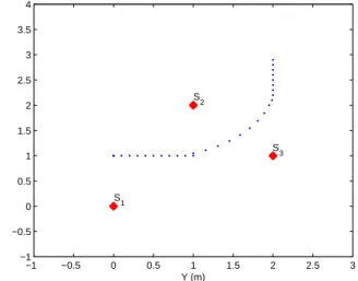
Application example

In this section a target tracking in a sensor network exam-ple presented in [8] is used to illustrated the state estima-tion method presented above. The problem consists of three sensors and one target moving in the horizontal plane. Each sensor can measure distance to the target, and by combining these a position fix can be computed. Fig. 1 depicts a sce-nario with a trajectory and a certain combination of sensor locations (S1, S2and S3). −1 −0.5 0 0.5 1 1.5 2 2.5 3 −1 −0.5 0 0.5 1 1.5 2 2.5 3 3.5 4 Y (m) S₁ S 2 S 3

Figure 1: Target true trajectory and sensor positions in the bounded horizontal plane

The behaviour of the system can be described by the fol-lowing discrete time state-space model:

( x1(k + 1) x2(k + 1) ) = ( x1(k) x2(k) ) + Ts ( v1(k) v2(k) ) (33)

( _y 1(k) y2(k) y3(k) ) =      √ (x1(k)− S1,1) 2 + (x2(k)− S1,2) 2 √ (x1(k)− S2,1)2+ (x2(k)− S2,2)2 √ (x1(k)− S3,1) 2 + (x2(k)− S3,2) 2      + ( _e 1(k) e2(k) e3(k) ) (34)

where x1(k) and x2(k) are the object coordinates bounded

by −1 ≤ x1(k) ≤ 3 and −1 ≤ x2(k) ≤ 4 ∀k ≥ 0.

Ts = 0.5s is the sampling time, v1(k) and v2(k) are the

speed components of the target that are unknown but con-sidered bounded by the maximum speed σv = 0.4m/s

(|v1(k)| ≤ σv and|v2(k)| ≤ σv). y1(k), y2(k) and y3(k)

are the distances measured by the sensors. Si,j denotes

the component j of the location of sensor i. e1(k), e2(k)

and e3(k) are the the stochastic measurement additive

er-rors pei ∼ N(0, σi) with σ1= σ2= σ3=

√

0.05m. Fig. 2 shows the evolution of the real sensor distances and measurements in the target trajectory scenario depicted in Fig. 1. 0 5 10 15 0 2 4 Distance 1 (m) Real Measured 0 5 10 15 0 0.5 1 1.5 Distance 2 (m) 0 5 10 15 0 1 2 3 Distance 3 (m) Time (s)

Figure 2: Real and measured distances from the target to the sensors

In order to apply the state estimation methodology pre-sented above, a minimum accuracy δ1 = δ2 = δ = 0.2m

has been selected for both components. No a priori infor-mation has been used in the initial state. Then, a uniform grid of disjoint boxes with the same weights and component widths ε1 = ε2 = δ that covers all the bounded

coordi-nates−1 ≤ x1 ≤ 3 and −1 ≤ x2 ≤ 4 has been chosen as

initial stateX (0). Posterior probabilities of the boxes have been approximated by weights w(k)i _{computed using the}

new sensor distances measurements in (4). State update has been computed considering speed bounds in (33). The new boxes have been rearranged considering the minimum ac-curacy δ and their associated weights have been computed using (4). Finally, Algorithm 2 with threshold γ = 1 has been applied to reduce the number of boxes.

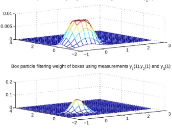
Figs. 3 and 4 depict the box weights and their contours using measurement y1(1) (up) and all the measurements at

−1 0 1 2 3 −2 0 2 40 0.005 0.01

Box particle filtering weight of boxes using measurement y

1(1) −1 0 1 2 3 −2 0 2 40 0.1 0.2

Box particle filtering weight of boxes using measurements y₁(1),y₂(1) and y₃(1)

Figure 3: Box weights using measurement y1(k) (up) and

measurements (y1(k), y2(k), y3(k))T (down) −1 −0.5 0 0.5 1 1.5 2 2.5 3 −1 0 1 2 3 4

Box particle filtering weight contour of boxes using measurement y

1(1) Real point Estimated BPF −1 −0.5 0 0.5 1 1.5 2 2.5 3 −1 0 1 2 3 4

Box particle filtering weight of boxes using measurements y₁(1),y₂(1) and y₃(1) Real point Estimated BPF

Figure 4: Box weight contours using measurement y1(k)

(up) and measurements (y1(k), y2(k), y3(k))T (down)

instant k = 1 (y1(1), y2(1) and y3(1)) (down). Fig. 5

de-picts the box weights and their contours using the measure-ments at hand at instant k = 2.

The real trajectory and the one estimated using (28) are shown in Fig. 6.

Finally, different additive sensor faults have been simu-lated and satisfactory results of the fault detection tests (30) and (32) have been obtained for faults bigger than 0.5m us-ing thresholds ∆ˆxmax and Λmin computed with (29) and (31)with L = 3200, β1= 1.1 and β2= 0.9.

Fig. 7 shows the real trajectory and the one estimated us-ing (28) when an additive fault of +0.5m affects sensor S1

at time k = 22. The behaviour of fault detection tests (30) and (32) is depicted in Fig. 8. As seen in this figure, both thresholds are violated at time instant k = 22 and therefore the fault is detected at this time instant.

−1 0 1 2 3 −2 0 2 40 0.1 0.2

Box particle filtering weight of boxes using available measurements at instant k=2

−1 −0.5 0 0.5 1 1.5 2 2.5 3 −1 0 1 2 3 4

Box particle filtering weight contour of boxes using available measurements at instant k=2 Real point

Estimated BPF

Figure 5: Box weights (up) and Box weights contours (down) at instant k = 2 −1 −0.5 0 0.5 1 1.5 2 2.5 3 −1 −0.5 0 0.5 1 1.5 2 2.5 3 3.5 4 x 1 (m) x2 (m) Real trajectory Box particle estimation

S 1 S 2 S₃ Figure 6: Trajectories

8

Conclusion and perspectives

A Box particle algorithm has been proposed for estimation and fault detection in the case of nonlinear systems with stochatic and bounded uncertainties. Using this method in the case of a target tracking sensor networks illustrates its feasibility. It has been shown how the measurement up-date state for the box particle is derived from the particle case. However convergence and stability of this filter have to be proved. Resampling unfortunatly drops information and waives guaranteed results that characterize interval analysis based solutions. However without resampling the particle filter suffers from sample depletion. This is the reason why resampling is a critical issue in particle filtering (Gustafsson 2002). This approach has to be compared to other PF vari-ants which reduce the number of particles [2] and further investigations concerning resampling are required, in par-ticular if we want to take better benefit of the interval based approach. −1 −0.5 0 0.5 1 1.5 2 2.5 3 −1 −0.5 0 0.5 1 1.5 2 2.5 3 3.5 4 x 1 (m) x2 (m) real

Box Particle Filter

Fault Detection S 2 S 1 S₃ k=21 k=22

Figure 7: Trajectories in fault scenario

5 10 15 20 25 30 0 0.2 0.4 0.6 ∆ ˆx ( k) Time (T_s=0.5s) 5 10 15 20 25 30 0 20 40 60 80 100 120 Λ (k) Time (T s=0.5s) Fault Detection Fault Detection

Figure 8: Fault indicators and thresholds in the fault sce-nario

Acknowledgments

This work is partially supported by CICYT ECOCIS DPI2013-48243-C2-1-R of the Spanish Ministry of Educa-tion and by 2014SGR374 of the Generalitat de Catalunya

A

Demonstration of Measurement update:

"From particles to boxes"

A.1

Particle filtering

j=1uniformly distributed in

x(k)j _{∈ [x(k), x(k)] ∀j = 1, . . . , N where x(k), x(k) ∈}

R. Then according to [1] the relative posterior probability for each particle is approximated by

P (x(k)j|Y(k)) ≈ 1

c(k)P (x(k)

j_|Y(k−1))p

e(y(k)−h(x(k)j))

with c(k) = N ∑ j=1 P (x(k)j|Y(k)) (36)

A.2

Grouping particles

If we group the N particles in Nggroups of ∆N elements

{x(k)j_}N j=1= Ng ∪ i=1 {x(k)l_}i∆N l=1+(i−1)∆N (37) with Ng= _∆NN

If we select the groups of points in such a way that

{x(k)l_}i∆N l=1+(i_−1)∆N ∈ [x(k)] i _{∀i = 1, . . . , N} g (38) where [x(k)]i= [x(k) + (i− 1)∆L, x(k) + i∆L] (39) with ∆L = x(k)− x(k) Ng (40) If the number of particles N → ∞ and therefore ∆N →

∞ P ([x(k)]i|Y(k)) ≈ i∆N∑ j=1+(i−1)∆N P (x(k)j|Y(k)) (41) according to (35) P ([x(k)]i|Y(k)) ≈ ∑i∆N

j=1+(i−1)∆NP (x(k)j|Y(k − 1))pe(y(k)− h(x(k)j))

∑Ng l=1

∑l∆N

j=1+(l−1)∆NP (x(k)j|Y(k − 1))pe(y(k)− h(x(k)j)) (42) If we consider the particles in the same group i have the same prior probabilities, then:

p(x(k)j|Y(k − 1)) = P ([x(k)]i_{|Y(k − 1))} ∆N ∀j = 1 + (i − 1)∆N, . . . , i∆N (43) and (42) leads to P ([x(k)]i|Y(k)) ≈

P ([x(k)]i|Y(k − 1))∑i∆N_{j=1+(i−1)∆N}pe(y(k)− h(x(k)j))

∑Ng

l=1(P ([x(k)]l|Y(k − 1))

∑l∆N

j=1+(l−1)∆Npe(y(k)− h(x(k)j))) (44) If the N particles are uniformly distributed in the interval [x(k), x(k)], i.e x(k)j− x(k)j−1= ∆x(k) ∀j = 2, . . . , N (45) where ∆x(k) =x(k)− x(k) N = ∆L ∆N (46) Then i∆N∑ j=1+(i−1)∆N pe(y(k)− h(x(k)j))∆x(k)≈ ∫ (i∆N )∆x(k) (1+(i_{−1)∆N)∆x(k)} pe(y(k)− h(x(k)))dx(k) ≈ ∫ x(k)∈[x(k)]i pe(y(k)− h(x(k)))dx(k) (47)

Finally, multiplying the numerator and denominator of equation (44) by ∆x, we obtain the particle box measure-ment update equation

P ([x(k)]i|Y(k)) ≈ P ([x(k)]i|Y(k − 1))∫_{x(k)∈[x(k)]}ipe(y(k)− h(x(k)))dx(k) ∑Ng l=1(P ([x(k)]l|Y(k − 1)) ∫ x(k)∈[x(k)]lpe(y(k)− h(x(k)))dx(k)) (48) that corresponds to the equation (11) with

Λ(k) = Ng ∑ l=1 (P ([x(k)]l|Y(k − 1)) ∫ x(k)∈[x(k)]l pe(y(k)− h(x(k)))dx(k)) (49)

References

[1] F. Gustafsson, F. Gunnarsson, N. Bergman, U. Forssell, J. Jansson, R. Karlsson, and P.J. Nordlund. Particle filters for positioning, navigation, and tracking.

Sig-nal Processing, IEEE Transactions on, 50(2):425–437,

2002.

[2] F. Abdallah, A. Gning, and P. Bonnifait. Box particle fil-tering for nonlinear state estimation using interval anal-ysis. Automatica, 44(3):807–815, 2008.

[3] A. Doucet, N. De Freitas, and N. Gordon. An

intro-duction to sequential Monte Carlo methods. Springer,

2001.

[4] A. Gning, L. Mihaylova, and F. Abdallah. Mixture of uniform probability density functions for non linear state estimation using interval analysis. In Information

Fusion (FUSION), 2010 13th Conference on, pages 1–

8. IEEE, 2010.

[5] R.M. Fernández-Cantí, S. Tornil-Sin, J. Blesa, and V. Puig. Nonlinear set-membership identification and fault detection using a bayesian framework: Applica-tion to the wind turbine benchmark. In Proceedings of

the IEEE Conference on Decision and Control, pages

496–501, 2013.

[6] J. Xiong, C. Jauberthie, L. Travé-Massuyès, and F. Le Gall. Fault detection using interval kalman filtering en-hanced by constraint propagation. In Proceedings of the

IEEE Conference on Decision and Control, pages 490–

495, 2013.

[7] A. Gning, B. Ristic, and L. Mihaylova. Bernoulli particle/box-particle filters for detection and tracking in the presence of triple measurement uncertainty. IEEE

Transactions on Signal Processing, 60(5):2138–2151,

[8] F. Gustafsson. Statistical sensor fusion. Studentlitter-atur, Lund, 2010.