The AMBRE project: Iron-peak elements in the solar neighbourhood

HAL Id: hal-03118590

https://hal.archives-ouvertes.fr/hal-03118590

Submitted on 22 Jan 2021

HAL is a multi-disciplinary open access

archive for the deposit and dissemination of

sci-entific research documents, whether they are

pub-lished or not. The documents may come from

teaching and research institutions in France or

abroad, or from public or private research centers.

L’archive ouverte pluridisciplinaire HAL, est

destinée au dépôt et à la diffusion de documents

scientifiques de niveau recherche, publiés ou non,

émanant des établissements d’enseignement et de

recherche français ou étrangers, des laboratoires

publics ou privés.

The AMBRE project: Iron-peak elements in the solar

neighbourhood

Š. Mikolaitis, P. de Laverny, A. Recio–blanco, V. Hill, C. C. Worley, M. de

Pascale

To cite this version:

Š. Mikolaitis, P. de Laverny, A. Recio–blanco, V. Hill, C. C. Worley, et al.. The AMBRE project:

Iron-peak elements in the solar neighbourhood. Astronomy and Astrophysics - A&A, EDP Sciences,

2017, 600, pp.A22. �10.1051/0004-6361/201629629�. �hal-03118590�

DOI:10.1051/0004-6361/201629629 c ESO 2017

Astronomy

&

Astrophysics

The AMBRE project: Iron-peak elements in the solar

neighbourhood

?

,

??

Š. Mikolaitis

1, 2

, P. de Laverny

2

, A. Recio–Blanco

2

, V. Hill

2

, C. C. Worley

3

, and M. de Pascale

4

1 _{Institute of Theoretical Physics and Astronomy, Vilnius University, Saul˙etekio al. 3, 10257 Vilnius, Lithuania}

e-mail: Sarunas.Mikolaitis@tfai.vu.lt

2 _{Université Côte d’Azur, Observatoire de la Côte d’Azur, CNRS, Laboratoire Lagrange, Bd de l’Observatoire, CS_34229,}

06304 Nice Cedex 4, France

3 _{Institute of Astronomy, University of Cambridge, Madingley Road, Cambridge CB3 0HA, UK}

4 _{INAF–Padova Observatory, Vicolo dell’Osservatorio 5, 35122 Padova, Italy}

Received 1 September 2016/ Accepted 24 November 2016

ABSTRACT

Context.The pattern of chemical abundance ratios in stellar populations of the Milky Way is a fingerprint of the Galactic chemical history. In order to interpret such chemical fossils of Galactic archaeology, chemical evolution models have to be developed. However, despite the complex physics included in the most recent models, significant discrepancies between models and observations are widely encountered.

Aims.The aim of this paper is to characterise the abundance patterns of five iron-peak elements (Mn, Fe, Ni, Cu, and Zn) for which the stellar origin and chemical evolution are still debated.

Methods.We automatically derived iron peak (Mn, Fe, Ni, Cu, and Zn) and α element (Mg) chemical abundances for 4666 stars, adopting classical LTE spectral synthesis and 1D atmospheric models. Our observational data collection is composed of high-resolution, high signal-to-noise ratios HARPS and FEROS spectra, which were previously parametrised by the AMBRE project.

Results.We used the bimodal distribution of the magnesium-to-iron abundance ratios to chemically classify our sample stars into different Galactic substructures: thin disc, metal-poor and high-α metal rich, high-α, and low-α metal-poor populations. Both high-α and low-α metal-poor populations are fully distinct in Mg, Cu, and Zn, but these substructures are statistically indistinguishable in Mn and Ni. Thin disc trends of [Ni/Fe] and [Cu/Fe] are very similar and show a small increase at supersolar metallicities. Also, both thin and thick disc trends of Ni and Cu are very similar and indistinguishable. Yet, Mn looks very different from Ni and Cu. [Mn/Fe] trends of thin and thick discs actually have noticeable differences: the thin disc is slightly Mn richer than the thick disc. The [Zn/Fe] trends look very similar to those of [α/Fe] trends. The typical dispersion of results in both discs is low (≈0.05 dex for [Mg, Mn, and

Cu/Fe]) and is even much lower for [Ni/Fe] (≈0.035 dex).

Conclusions.It is clearly demonstrated that Zn is an α-like element and could be used to separate thin and thick disc stars. Moreover,

we show that the [Mn/Mg] ratio could also be a very good tool for tagging Galactic substructures. From the comparison with Galactic

chemical evolutionary models, we conclude that some recent models can partially reproduce the observed Mg, Zn, and, Cu behaviours in thin and thick discs and metal-poor sequences. Models mostly fail to reproduce Mn and Ni in all metallicity domains, however, models adopting yields normalised from solar chemical properties reproduce Mn and Ni better, suggesting that there is still a lack of realistic theoretical yields of some iron-peak elements. The very low scatter (≈0.05 dex) in thin and thick disc sequences could provide an observational constrain for Galactic evolutionary models that study the efficiency of stellar radial migration.

Key words. Galaxy – stars: abundances – Galaxy: stellar content – star: abundances

1. Introduction

The pattern of chemical abundances directly reflect the history of a stellar population. The main contributors to the interstellar medium chemical evolution are believed to be asymptotic gi-ant branch (AGB) stars and type-Ia and type-II supernovae. The final picture of stellar abundances in the Galaxy is thus prede-termined by a complex interplay of several mechanisms: a su-pernovae type that was predominant in the region of the stel-lar nursery, the typical mass of type-II supernovae when stars formed, the timing of the mechanism that switched on the type-Ia

? _{Based on observations collected at ESO telescopes under the}

AMBRE programme.

?? _{Full Table5is only available at the CDS via anonymous ftp to}

cdsarc.u-strasbg.fr(130.79.128.5) or via

http://cdsarc.u-strasbg.fr/viz-bin/qcat?J/A+A/600/A22

supernovae, and the amount of contamination in the region by supernovae and AGB ejecta. This information is important to un-locking the knowledge of the formation and evolution histories of our Galaxy. Among the numerous observational properties that are usually collected to describe the Galactic populations, one of the most powerful properties consists in collecting chem-ical abundance ratios between different key elements. Then, such ratios in the different Galactic components have to be inter-preted together with other signatures (such as kinematical sig-natures, for instance) by chemical models of the Milky Way. Obviously, the solar vicinity is the most studied region of the Milky Way and several chemical evolution models have been developed to explain the chemical composition of the local disc (e.g.Chiappini et al. 2003b,a;François et al. 2004). However, most of these studies typically modelled the solar vicinity as one merged system without reproducing the chemical patterns

of Galactic substructures. Nevertheless, there are several more recent models (Kobayashi et al. 2006; Kobayashi & Nakasato 2011; Romano et al. 2010; Kubryk et al. 2015) that aimed to reproduce most of the chemical abundance patterns of the four main Galactic components (bulge, halo, thin, and thick discs) for elements up to Z= 30. Although such Galactic chemical evolu-tion models are very complex and advanced, one could still see that part of the chemical patterns found in the solar neighbour-hood are still not well understood.

With this paper, we aim to better describe the behaviour of the manganese, nickel, copper, and zinc elements in the Galaxy. We chose these iron-peak chemical species since they are key products of stellar nucleosynthesis.

Manganese (55Mn) is produced during thermonuclear ex-plosive silicon burning and α-rich freeze-out via synthesis of

55_{Co. These reactions are active in type-Ia (Bravo 2013) and}

type-II (Woosley & Weaver 1995) supernovae, although these reactions are thought to be produced more by type-Ia supernovae than by hypernovae or type-II supernovae (Iwamoto et al. 1999;

Kobayashi & Nomoto 2009). However, it is still under debate whether the manganese-to-iron trends behave differently in thin and thick discs at similar metallicities, probably revealing di ffer-ent evolution histories (Feltzing et al. 2007;Hawkins et al. 2015;

Battistini & Bensby 2015). Nickel is also produced by the silicon burning process. However, yields from type-Ia and type-II super-novae are comparable. Thus nickel behaves almost like iron from an observational point of view. However, it is still very difficult for Galactic models to match the observed nickel behaviour in the Milky Way. Copper is an odd iron-peak element and its ori-gin is still not well understood. For example, it is thought that solar copper is mostly the outcome of weak s and r processes (Bisterzo et al. 2004). However, there are other nucleosynthesis channels known for copper, but their relative contributions are under debate (Bisterzo et al. 2006). Finally, in massive stars most of the zinc should have been produced by similar nucleosynthe-sis channels such as copper, but with different contribution ra-tios.64_{Zn is mostly produced from α-rich freeze-out in γ winds}

and (66,67,68,70_{Zn) is produced by the sr process. Other}

contribu-tions are marginal (Bisterzo et al. 2004,2006). The zinc-to-iron ratio pattern should resemble that of the α elements. However, such a behaviour is still not explicitly modelled or confirmed by observations based on large Galactic samples.

Indeed, large and homogeneous samples of Mn, Ni, Cu, and Zn abundances are required in order to better understand the evo-lution of these elements in our Galaxy and to test the quality of chemical evolution models. Although there are already some significant samples of Mn, Ni, Cu, and Zn abundances derived from high-resolution spectra, the size and completeness of these samples vary a lot from element to element. For instance, the largest uniform samples of manganese and nickel abundances were provided by Adibekyan et al. (2012; 1111 dwarf stars),

Bensby et al. (2014; 714 dwarfs), Battistini & Bensby (2015; 596 dwarfs), andHawkins et al.(2015; 3200 giants). However, copper and zinc have been given less attention in observational studies. The largest samples of Cu were studied by Reddy & Lambert(2008; uniform sample of 181 stars) andBisterzo et al.

(2006; non-uniform collection of abundances for more than 300 stars). There exists only one uniform and large sample re-porting zinc abundances (Bensby et al. 2014, 714 dwarf stars), whereasBisterzo et al.(2004) collected a non-uniform sample of more than 300 stars.

In order to increase the size of observed samples for iron-peak elements by about one order of magnitude, in this article we present a very large catalogue of homogeneous magnesium,

manganese, iron, nickel, copper, and zinc elemental abundances derived for 4666 slow-rotating stars. Our sample contains stars in various evolutionary stages and covers a large metallicity do-main in the different Galactic components. This study is part of the Galactic Archaelogy AMBRE project relying on archived ESO spectra (de Laverny et al. 2013). In Sect.2, we describe the observational data sample and the method adopted to derive the chemical abundances. Section3is devoted to tagging the anal-ysed stars to the different Galactic components based on their enrichment in magnesium. In Sect.4, we describe the behaviour of the iron-peak elements in these different Galactic disc compo-nents. In Sect.5, we compare our observational results with re-cent Galactic chemical evolution models. Finally, we summarise and conclude our work in Sect.6.

2. The AMBRE catalogue of iron-peak elements

2.1. Stellar sample and atmospheric parameters

For the present study, we adopted the AMBRE project data that are described in de Laverny et al. (2013) and consist in the automatic parametrisation of large sets of ESO high-resolution archived spectra. Within the AMBRE project,the stellar atmo-spheric parameters (in particular, Teff, log g, [M/H], and [α/Fe]

together with their associated errors) were derived using the MATISSE algorithm (Recio-Blanco et al. 2006). For the present study, we adopted the data of the FEROS and HARPS spectro-graphs (hereafter AMBRE:FEROS and AMBRE:HARPS sam-ples). The complete parametrisation of the AMBRE:FEROS spectra has been performed by Worley et al. (2012, hereafter W12) for 6508 spectra, whereas the 90 174 AMBRE:HARPS spectra have been fully parametrised byDe Pascale et al.(2014, hereafter dP14).

For some stars, these two samples (and particularly the HARPS sample) contain a large number of repeated observa-tions. The actual number of targeted stars is thus smaller than the number of parametrised spectra. As already shown in W12, the number of AMBRE:FEROS stars is actually 3087 as defined by their coordinates. For the AMBRE:HARPS sample, the ac-tual number of stars has been calculated by, first, analysing the spectra in a 3D space (RA, Dec, and radial velocity). For that purpose, we selected every spectra found within a radius of 500

and look for clusters in the radial velocity (Vrad). We defined in-dependent clusters as spectra with Vrad departing by more than 2σ from the mean Vrad value of the cluster. Then, we checked the atmospheric parameters to disentangle stars within a cluster. We thus made the so-called single linkage cluster analysis for well-separated clusters to search for the statistical clusterisation of solutions in a 4D space (Te_ff, log g, [M/H], and [α/Fe]). If all

4D parameters of one cluster of solutions were different from an-other cluster by at least 2σ in the parameter values, we accepted this solution as a single star. In such a way, we found 5049 in-dividual stars in the AMBRE:HARPS sample. Moreover, if a given star did not have a single observation with CHI2_FLAG=0 (quality flag of the fit between the observed and reconstructed synthetic spectra with the AMBRE parameters, zero meaning very good fit), this star was omitted from further analysis. This procedure led to a AMBRE:HARPS sample with 4355 stars and to a AMBRE:FEROS sample with 1925 stars.

For the chemical analysis presented in Sect.2.2and in case of repeats within one of these two samples, we selected one spectrum per star by favouring the best combination of AMBRE CHI2 and signal-to-noise ratio (S/N) values. The CHI2 is the log (χ2_{) fit between the observed spectrum and the synthetic}

spectrum reconstructed with the AMBRE atmospheric parame-ters. The S/N is a signal-to-noise ratio estimated by the AMBRE pipeline (see Table A.1 in W12 and Table 2 in dP14 for details). In case of multiple observations of the same star (ten or more), we first selected five spectra with the best S/N. Then, among these spectra, we selected the spectrum with the highest CHI2 value. If the number of repeats is rather small (∼10), we simply selected the spectrum with the best S/N.

Finally, we also found that there are 320 stars in common between the final AMBRE:FEROS and AMBRE:HARPS sam-ples; this was checked by coordinates, radial velocities, and at-mospheric parameters. The comparison between FEROS and HARPS stellar parameters and abundances for 320 stars in com-mon is shown in Fig. 1. Therefore, even if a small dispersion and bias are present for some stellar parameters, they do not affect the derived [El/Fe] abundance ratios. We then consid-ered only the HARPS spectra for our final analysis since they usually have higher S/N values and higher spectral resolution. We therefore have a final catalogue of 5960 (4355 HARPS and 1605 FEROS) individual slow-rotating stars (and spectra) homo-geneously parametrised by the AMBRE project.

2.2. Chemical abundance analysis 2.2.1. Adopted methodology

The method used to derive individual chemical abundances of Mg, Mn, Fe, Ni, Cu, and Zn is described in Mikolaitis et al.

(2014). Here we briefly describe the most relevant informa-tion. We adopted the AMBRE atmospheric parameters (Teff,

log g, h[M/H]i, and [α/Fe]) to derive the chemical abundances. We use the notation [M/H] for the metallicity of the atmo-spheric model and the value derived by the AMBRE Project. For the neutral and ionised iron abundances, we use the notations [Fe

_i

/H] and [Fe

_ii

/H]. Similarly, [α/Fe] refers to the α to iron ratio of the atmospheric model derived by AMBRE. We com-puted the microturbulent velocity using the fixed function of Teff,

log g, and [M/H] as defined within the Gaia-ESO Survey (GES) (Bergemann et al., in prep.). We also kept the original spectral resolution for the analysis, i.e. around 48 000 and 120 000 for FEROS and HARPS, respectively. These spectral resolutions are much larger than that adopted by the AMBRE Project for the stellar parametrisation.

As for the atomic line selection of the considered chemical species, we first look for lines that can be found in both spec-tral domains covered by the FEROS and HARPS instruments. Then, to consider the best possible line data, we looked at the lines provided by the Gaia-ESO Survey line list group (Heiter et al. 2015). Atomic lines that were selected for the abundance analysis are presented in Table1. Iron lines are too numerous (139 in total) to be presented in Table 1, but we confirm that these lines are typically used in stellar spectroscopy since they are well observed in solar or Arcturus spectra (seeSousa et al. 2014, for instance). Some types of stars were slightly sensitive to molecular absorption, thus it was necessary to use molecular line lists kindly provided by T. Masseron for C2(Brooke et al. 2013;

Ram et al. 2014), CN (Sneden et al. 2014), OH (Masseron, priv. comm.), MgH (Masseron, priv. comm.), CH (Masseron et al. 2014), CaH (Plez, priv. comm.), NH (Masseron, priv. comm.), SiH (Kurucz 1993), and FeH (Dulick et al. 2003).

Regarding the normalisation of the observed spectra, our chemical analysis pipeline determines the continuum level in two steps. First, we employed the DAOSPEC tool (Stetson & Pancino 2008) to estimate the continuum function over the whole

Table 1. Lines (λ(Å)) used for the analysis.

Mgi 5167.3 5172.6 5183.6 5528.4 5711.0 6318.7 6319.2 6319.4 Mni 4783.4B _4823.5B _5004.9BW _5117.9J _5255.3J _5394.7D 5407.4De 5420.4De 5432.5D 5516.8De 6013.5H 6016.7H 6021.8H _6440.9H Nii 4811.9 4814.5 4873.4 4953.2 4976.1 4976.3 4976.6 5003.7 5035.3 5137.0 5157.9 5424.6 5435.8 5578.7 5587.8 5709.5 5846.9 6108.1 6128.9 6176.8 6204.6 6223.9 6230.0 6327.5 6378.2 6384.6 6414.5 6482.7 6643.6 6767.7 Cui 5105.5F 5153.2 5218.2He 5220.1He 5700.2Be 5782.1Be Zni 4722.1 4810.5 6362.3

Notes. HFS data from: (B) _{Brodzinski et al. (1987);}

(BW) _{Blackwell-Whitehead et al.(2005);} (J) _{Johann et al. (1981);} (D) _{Davis et al.(1971);}(De) _{Dembczy´nski et al. (1979);}(H) _Handrich

et al. (1969); (F) _{Fischer et al. (1967);} (He) _{Hermann et al. (1993);} (Be)_{Bergström et al.(1989).}

spectrum. We used this function as a first guess of the con-tinuum. Then we adjusted the continuum locally in the region (±5 Å) around every line of interest. This was carried out by selecting the possible line-free zones of the normalised syn-thetic spectrum, defined as regions where the intensity of the synthetic spectrum is depressed by less than 0.02%. If the pos-sible line-free zones are too narrow or do not exist for cer-tain types of stars, we iteratively searched for the possible less contaminated zones in the synthetic spectrum. We adopted interpolated MARCS (Gustafsson et al. 2008) model atmo-spheres and the version v12.1.1 of the spectrum synthesis code TURBOSPECTRUM (Alvarez & Plez 1998) for all spectral syn-thesis.

Then, the abundance analysis was divided into two indepen-dent steps after having performed the radial velocity correction, adopting the AMBRE Vrad.

First, we estimated the average line broadening for each star; the spectral line broadening is mainly caused by stellar rotation (v sin i). However, lines are also broadened by veloc-ity fields in the stellar photosphere known as macroturbulence (vmac). Unfortunately, disentangling the rotational profile from

the radial-tangential vmacprofile is difficult, leading to a

degener-acy between both quantities measured (Doyle et al. 2014). Thus, we assume in the following that the line broadening parameter corresponds to the rotational velocity keeping in mind that there is a small influence of the vmacprofile. We note that the AMBRE

Project focuses on slow-rotating stars only (up to ∼20 km s−1). The v sin i of each star was measured together with their iron [FeI/H] and [FeII/H] abundances, which could differ slightly from the AMBRE mean metallicity [M/H]. We then computed the individual chemical abundances adopting the derived v sin i.

The v sin i was adjusted iteratively by minimising the χ2 _of

the fit between the synthetic spectrum and observed spectrum around some specific lines. We chose to adjust v sin i using neu-tral iron lines (up to 139 are available in the analysed specneu-tral domains) because (i) we were able to adopt the AMBRE metal-licity as a first guess of the iron abundance; and (ii) iron lines are the most numerous. First, for a given spectrum and iron line, we created a grid of synthetic spectra with different v sin i values

4500 5000 5500 6000 6500 -300 0 300 2 3 4 5 -1.0 -0.5 0.0 0.5 1.0 -2 -1 0 1 -1.0 -0.5 0.0 0.5 1.0 -100 0 100 -5 0 5 4500 5000 5500 6000 6500 -0.4 -0.2 0.0 0.2 0.4 4500 5000 5500 6000 6500 -0.4 -0.2 0.0 0.2 0.4 4500 5000 5500 6000 6500 -0.4 -0.2 0.0 0.2 0.4 4500 5000 5500 6000 6500 -0.4 -0.2 0.0 0.2 0.4 4500 5000 5500 6000 6500 -0.4 -0.2 0.0 0.2 0.4 4500 5000 5500 6000 6500 -0.4 -0.2 0.0 0.2 0.4 T e ff F E R O S T e ff H A R P S ( K ) Teff HARPS (K)

Teff = 23 K, (Teff)= 53 K log(g) = 0.14, (log(g)) = 0.12 [M/H] = 0.02, ([M/H]) = 0.10 RV = -0.01 km/s, ([M/H]) = 0.31 km/s

l o g ( g ) F E R O S l o g ( g ) H A R P S log(g) HARPS [ M / H ] F E R O S [ M /H ] H A R P S [M/H] HARPS R V F E R O S -R V H A R P S ( km / s) RV HARPS (km/s) [Mg/Fe] = 0.02, ([Mg/Fe]) = 0.05 [ M g / F e ] F E R O S -[ M g / F e ] H A R P S Teff HARPS (K) [Mn/Fe] = 0.01, ([Mn/Fe]) = 0.04 [ M n / F e ] F E R O S -[ M n / F e ] H A R P S Teff HARPS (K) [Ni/Fe] = 0.00, ([Ni/Fe]) = 0.04 [ N i / F e ] F E R R O S -[ N i/ F e ] H A R P S Teff HARPS (K) [Cu/Fe] = 0.01, ([Cu/Fe]) = 0.04 [ C u / F e ] F E R O S -[ C u / F e ] H A R P S Teff HARPS (K) [M/H] = 0.02, ([/Fe]) = 0.04 [Zn/Fe] = 0.01, ([Zn/Fe]) = 0.04 [ Z n / F e ] F E R O S -[ Z n /F e ] H A R P S Teff HARPS (K) [ / F e ] F E R O S -[ /F e ] H A R P S [M/H] HARPS

Fig. 1.Comparison between the stellar parameters derived by the AMBRE:FEROS and the AMBRE:HARPS pipeline (top five plots); comparison

between [El/Fe] abundance ratios (lower five plots) for 320 stars in common between the final AMBRE:FEROS and AMBRE:HARPS samples.

Fig. 2.Rotational velocity distribution in bins of∆v sin i = 2 km s−1_.

The grey vertical line indicates the selection cut-off at v sin i =

10 km s−1_.

(from v sin i = 0.0 to 20.0 km s−1with a step 0.1 km s−1) and searched for the best fit (lowest χ2). Then, we adopted this cho-sen v sin i as a first guess to compute the iron abundance of the specific line; see below for a short description of the methodol-ogy adopted for the chemical analysis. We repeated those two steps until convergence on both v sin i and [Fe/H] was reached for the specific iron line studied. Finally, we computed the mean and scatter of v sin i, excluding iron lines that were too weak as defined by their line depth (i.e. excluding lines with a line depth smaller than twice the noise level). We point out that the num-ber of lines available for this v sin i estimation varies from star to star. On average, we used 98 iron lines; this number varies from 29 in very metal-poor stars to 139 in metal-rich, high S/N spectra. The derived iron abundances ([FeI/H] and [FeII/H]) are presented in Sect. 2.3together with their comparison with the AMBRE [M/H] mean metallicity.

As shown in Fig.2, most of the sample stars are slow ro-tators (v sin i < 10 km s−1 for 86% of the sample, hv sin ii = 5.1 km s−1). This confirms the assumption adopted within the AMBRE Project to reject spectra with rotational velocity that is too high (actually, high values of the full width at half maxi-mum (FWHM) of the cross-correlation function (CCF) between the spectra and binary masks), with a limit around v sin i ∼ 15 km s−1.

In the following, and in order to consider only spectra with accurate atmospheric parameters derived by the AMBRE pipeline that relies on a grid of non-rotating spectra, we per-formed the chemical analysis only for the stars with v sin i < 10 km s−1. This very strict criterion rejected 987 stars from the original sample leading to a final sample of 4973 stars (with FEROS or HARPS spectra).

For these stars, we determined the LTE Mg

_i

, Mn

_i

, Ni

_i

, Cu

_i

, and Zn

_i

abundances (in addition to Fe

_i

and Fe

_ii

) by the same line-fit method as inMikolaitis et al.(2014) using previously de-rived v sin i and the AMBRE atmospheric parameters (Teff, log g,

[M/H], and [α/Fe]). We point out that because of the lack of NLTE correction tables available for all the studied species, all forthcoming discussions are based on the derived LTE abun-dances. However, some possible NLTE deviations have already been estimated in previous works. For instance,Mishenina et al.

(2015) observed average LTE-NLTE abundance variations of 0.01 ± 0.04 and 0.02 ± 0.04 dex for the thin and thick discs, re-spectively. Our LTE determinations for the Mn abundance can be accepted within the given uncertainty of 0.1 dex and the NLTE effect for this element cannot affect our discussion about thin and discs. We reach a similar conclusion about the NLTE ef-fect for Cu abundances sinceShi et al. (2014) and Yan et al.

(2016) have shown that the NLTE-LTE deviations for typical thin and thick disc stars are generally small (up to 0.1 dex for [Fe/H] ≈ –1.0 dex). Moreover,Yan et al.(2016) have shown in their Fig. 2 and similar samples as ours that the Cu NLTE ef-fects should not affect our discussion. Also, we point out, that the Zn

_i

6362 line suffers from Ca

_i

auto-ionisation broad absorp-tion feature as identified byMitchell & Mohler(1965). However,

Chen et al.(2004) showed that differentially with respect to the Sun, the largest effect from this auto-ionisation line would then be a decrease of [Zn/Fe] for the most metal-poor stars by only about 0.02 dex. Typically, our combined errors are significantly larger than this possible error contribution, which has thus been neglected in the present analysis.

2.2.2. Error estimation for the chemical abundances

The different sources of error impacting the chemical abun-dances are described inMikolaitis et al.(2014). We briefly dis-cuss these in the following.

The first category of errors includes those affecting a single line (e.g. random errors of the line fitting or continuum place-ment). The second category includes the errors affecting all lines. One way (see also the item 1 below) to evaluate this sort of error is to select a statistically significant set of spectra of the same object (repeats) with different S/N, and then to evaluate

the dispersion of the results. Another way is to follow the line-to-line scatter (see also the item 2 below). Finally (see also the item 3), we studied the propagation of the errors from the atmo-spheric parameters (Teff, log g, [M/H], and vt) to the chemical

abundances. These error analyses are presented below.

1. Error evaluation using object repeats. The present project benefits from the large number of repeated observations of the same star (particularly for the HARPS sample). As a con-sequence, we are able to select a large number of spectra targeting the same stars observed during different observa-tional conditions and covering a large domain of S/N values. The selected stars (dwarf and giants, metal-rich and poor), their number of available spectra and the estimated disper-sions (σ) on the derived chemical abundances are presented in Table2. We point out that the effects induced by differ-ences in the continuum normalisation are included in the es-timated dispersions. One can see that the eses-timated disper-sions are always very small (a couple of hundredths of dex) for every tested star and any chemical species.

2. Error evaluation according line-to-line scatter. We provide such scatter estimates for all elements in Table3, where hσi is the mean and σmaxis the maximum of the standard

devia-tion for a given element. These errors are very small and we adopted the values of Table3(hσi) in the estimation of the total error budget.

3. Propagation of the uncertainties on the main atmospheric parameters. The typical errors on the atmospheric pa-rameters are provided by the AMBRE Project. For the AMBRE:HARPS sample (De Pascale et al. 2014) they are: ∆Teff ≈ 93 K,∆logg ≈ 0.26 dex, and ∆[M/H] ≈ 0.08 dex.

For the AMBRE:FEROS sample (Worley et al. 2012) they are: ∆Teff ≈ 120 K, ∆log g ≈ 0.37 dex (if log g < 3.2),

∆log g ≈ 0.20 dex (if log g ≥ 3.2), and ∆[M/H] ≈ 0.10 dex. The adopted errors of∆vt are ≈0.3 m/s for both samples.

The impact of errors of the atmospheric parameters on the derived abundances are reported in Table4. We first provide the typical errors (Cols. 2 to 5) from errors on Teff, log g,

[M/H], and vt separately. Then, the combination of these

four contributions has been summed in quadrature (Col. 6), thus providing a conservative estimate of the error bar, which is probably slightly overestimated since the covariance be-tween the stellar parameters has been neglected. However, one should expect that the errors in the [X/H] abundance dif-fer from those of the [X/Fe] ratios, since in many cases the effect of changing the stellar parameters is similar for lines of different elements. Thus, the [X/Fe] ratio is often less sen-sitive to stellar parameter uncertainties. The error budget in the [X/Fe] scale therefore is reported in Col. 7, confirming that σtotal([X/H])is larger than σtotal([X/Fe])for every species.

Finally, the total error budget has been estimated by taking into account the errors from stellar parameter uncertainties as well as random errors. We thus calculated σall([X/Fe]) (Table4,

Col. 8) for every given element of every given star as

σall([X/Fe])= s σ2 total([X/Fe])+ σN √ N !2 ,

where σNis the line-to-line scatter and N is the number of

anal-ysed atomic lines. If the number of lines is N = 1, we adopted hσi from Table3for a given element as σN. The typical errors

(in [X/Fe]) for the abundances are between 0.03 and 0.12 dex, but most of these errors are smaller than 0.07 dex.

Table 2. Mean and dispersion of atmospheric parameters, signal-to-noise ratios and the derived chemical abundances for repeated spectra.

Line Mean σ Mean σ

HARPS HD 188512 (1033∗) HD 190248 (1160) Teff 5132.56 54.26 5567.14 3.77 log g 3.53 0.11 4.21 0.00 [M/H] –0.27 0.01 0.30 0.00 S/N 123.80 36.73 99.9 38.39 [Mg

_i

/M] 0.07 0.00 –0.0 0.00 [Fe

_i

/M] –0.13 0.03 –0.15 0.01 [Fe

_ii

/M] 0.04 0.01 –0.01 0.00 [Mn

_i

/M] –0.02 0.01 –0.08 0.00 [Ni

_i

/M] 0.03 0.01 0.04 0.01 [Cu

_i

/M] 0.01 0.03 0.02 0.04 [Zn

_i

/M] –0.14 0.04 –0.22 0.02 HD 31128 (47) HD 11977 (181) Teff 5807.10 37.14 4970.80 33.10 log g 3.97 0.05 2.46 0.03 [M/H] –1.74 0.01 –0.31 0.03 S/N 81.7 28.38 52.6 54.85 [Mg

_i

/M] 0.37 0.00 0.17 0.00 [Fe

_i

/M] 0.23 0.03 0.16 0.01 [Fe

_ii

/M] 0.24 0.01 0.11 0.00 [Mn

_i

/M] –0.32 0.01 0.19 0.00 [Ni

_i

/M] –0.09 0.01 0.12 0.01 [Cu

_i

/M] –0.31 0.03 0.28 0.04 [Zn

_i

/M] 0.17 0.04 0.15 0.02 FEROS HD 217107 (107) HD 156384B (38) Teff 5624.31 7.49 4648.78 8.90 log g 4.44 0.00 4.60 0.01 [M/H] 0.25 0.01 –0.47 0.00 S/N 66.26 22.97 96.75 20.01 [Mg

_i

/M] 0.18 0.02 0.16 0.01 [Fe

_i

/M] 0.17 0.02 0.04 0.01 [Fe

_ii

/M] 0.17 0.01 0.04 0.01 [Mn

_i

/M] 0.12 0.02 0.04 0.04 [Ni

_i

/M] 0.23 0.01 0.06 0.01 [Cu

_i

/M] 0.23 0.01 0.12 0.01 [Zn

_i

/M] 0.08 0.02 0.11 0.04 HIP 11952 (26) HD 10042 (25) Teff 5866.41 15.68 4903.90 20.04 log g 3.65 0.05 2.59 0.06 [M/H] –1.93 0.04 –0.44 0.05 S/N 78.26 28.75 67.34 30.50 [Mg

_i

/M] 0.43 0.02 0.51 0.01 [Fe

_i

/M] 0.35 0.02 0.21 0.01 [Fe

_ii

/M] 0.27 0.01 0.12 0.01 [Mn

_i

/M] 0.12 0.02 0.03 0.04 [Ni

_i

/M] –0.05 0.01 0.16 0.01 [Cu

_i

/M] –0.23 0.01 0.26 0.01 [Zn

_i

/M] 0.32 0.02 0.41 0.04

Notes. The numbers in parenthesis refers to the number of analysed

Table 3. Mean line-to-line scatter when two or more lines are available.

Line hσi σmax∗ Nmax∗∗

[Mg

_i

/H] 0.02 0.05 8 [Mn

_i

/H] 0.03 0.05 14 [Fe

_i

/H] 0.04 0.07 139 [Fe

_ii

/H] 0.02 0.07 11 [Ni

_i

/H] 0.03 0.05 30 [Cu

_i

/H] 0.03 0.07 6 [Zn

_i

/H] 0.02 0.07 3

Notes.(∗)_{Largest line-to-line scatter when two or more lines are}

avail-able.(∗∗)_N

maxis the maximum number of available lines.

2.3. The final catalogue

The metallicity value ([M/H]) derived by AMBRE corresponds to the mean metallicity of a star. However, we also derived the Fe

_i

and Fe

_ii

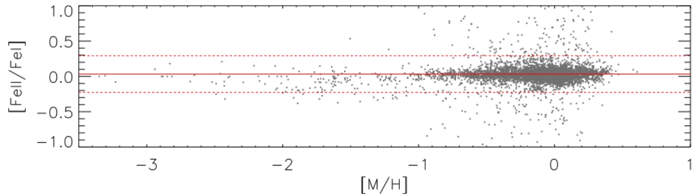
abundances in the present work. Since this mean metallicity and these iron abundances were computed in dif-ferent and slightly independent ways, it is important to check whether they are consistent between each other. We thus provide this comparison in Fig.3. First, the bias of [Fe

_i

/H] according to [M/H] is +0.072 dex with a scatter σ = 0.10 dex. For metal-poor stars, we detect slightly higher Fe

_i

abundances than for metal-rich stars. We did not detect any other notable systematic effects (regarding for instance some dependencies with stellar parameters).

Secondly, Fig.4compares the neutral and ionised iron abun-dances to check the ionisation equilibrium. We detect a very small bias (0.033 dex) for [Fe

_ii

/Fe

_i

] and a scatter σ= 0.13 dex. One can see that ionisation equilibrium is better preserved for metal-rich stars (for which the NLTE effects are believed to be smaller). For metal-poor stars ([M/H] < –1.0 dex) the [Fe

_ii

/Fe

_i

] values are lower by about 0.101 dex. Obviously, NLTE effects are significantly stronger for metal-poor stars, but the prime ef-fect is over-ionisation. However, our metal-poor stars are mostly giants (Teff < 5250 K, log g < 3.5) for which the gravity is

derived with larger uncertainties. Anyway, the detected small, unbalanced ionisation equilibrium and stronger drift of [Fe

_i

/H] from [M/H] could be caused by some NLTE effects and larger uncertainties of atmospheric parameters, especially for these metal-poor stars.

On the other hand, there are some stars that depart in [Fe

_i

/M] by more than 2σ with respect to the mean [Fe

_i

/M] at a given metallicity. Also there are some stars for which the ionisation balance is not preserved (|[Fe

_ii

/Fe

_i

]−h[Fe

_ii

/Fe

_i

]i| > 2σ). To avoid any spurious effect on abundances, we decided that, if at least one of these two conditions is not preserved for a given star, it is rejected from further analysis and from the final catalogue.

As a consequence, we omitted 987 stars from the primary list of 5960 because of our v sin i criteria and 307 additional stars because of the M-FeI-FeII test. The cool portion of the main se-quence (Teff < 4500 K and log g < 4.25) shows slightly lower

gravity than expected (log g > 4.3) as already pointed out by several independent analyses (e.g. within the Gaia-ESO survey). All stars (62) that show very large (more than 0.5 dex) positive or negative [Fe

_i

/M] and [Fe

_ii

/Fe

_i

] belong to that cool main-sequence potion. As already pointed out byWorley et al.(2012), one of the (several) causes of this problem could be the normal-isation procedure that may not be as robust for these cool stars. We also checked whether this issue could affect the individual chemical abundances, and we confirmed that the [X

_i

/Fe] ratios

Table 4. Effects on the derived abundances ([X/H]), resulting from the atmospheric parameters uncertainties for four types of stars, selected by

Teff, and log g.

El ∆Teff ∆log g ∆[M/H] ∆vt σtotal[X

H] σtotal[FeX] σall[FeX] Teff < 5000 K, log g < 3.5 Mg

_i

0.08 0.11 0.03 0.03 0.15 0.08 0.10 Mn

_i

0.06 0.01 0.01 0.03 0.07 0.04 0.05 Fe

_i

0.05 0.06 0.07 0.02 0.11 0.06 0.07 Fe

_ii

0.08 0.11 0.02 0.04 0.15 0.08 0.10 Ni

_i

0.03 0.04 0.02 0.02 0.06 0.03 0.04 Cu

_i

0.12 0.10 0.08 0.04 0.18 0.10 0.12 Zn

_i

0.11 0.09 0.09 0.04 0.17 0.10 0.11 Teff > 5000 K, log g < 3.5 Mg

_i

0.07 0.10 0.02 0.03 0.12 0.07 0.08 Mn

_i

0.07 0.01 0.01 0.03 0.08 0.04 0.05 Fe

_i

0.07 0.10 0.09 0.02 0.16 0.09 0.10 Fe

_ii

0.02 0.08 0.01 0.04 0.09 0.05 0.06 Ni

_i

0.07 0.02 0.01 0.02 0.08 0.04 0.05 Cu

_i

0.08 0.02 0.02 0.04 0.09 0.05 0.06 Zn

_i

0.03 0.04 0.03 0.04 0.08 0.04 0.05 Teff < 5000 K, log g > 3.5 Mg

_i

0.05 0.09 0.04 0.04 0.11 0.06 0.07 Mn

_i

0.03 0.03 0.01 0.03 0.05 0.03 0.03 Fe

_i

0.07 0.05 0.08 0.02 0.12 0.07 0.08 Fe

_ii

0.10 0.09 0.02 0.03 0.14 0.08 0.09 Ni

_i

0.01 0.05 0.02 0.03 0.06 0.03 0.04 Cu

_i

0.03 0.06 0.02 0.04 0.08 0.04 0.05 Zn

_i

0.06 0.05 0.04 0.04 0.10 0.06 0.07 Teff > 5000 K, log g > 3.5 Mg

_i

0.04 0.04 0.03 0.03 0.09 0.05 0.06 Mn

_i

0.03 0.03 0.01 0.02 0.04 0.02 0.03 Fe

_i

0.06 0.05 0.07 0.02 0.09 0.05 0.06 Fe

_ii

0.09 0.07 0.02 0.03 0.11 0.06 0.07 Ni

_i

0.01 0.03 0.02 0.03 0.06 0.03 0.04 Cu

_i

0.03 0.05 0.02 0.03 0.07 0.04 0.05 Zn

_i

0.05 0.05 0.03 0.04 0.09 0.05 0.06

Notes. The table shows the median of the propagated errors on [X/H]

ratios due to∆Teff,∆log g, ∆[M/H], ∆vt. The σtotal([X/H])stands for the

median of the quadratic sum of all four effects on [X/H] ratios. The σtotal([X/Fe])stands for the median of the quadratic sum of all four effects

on [X/Fe] ratios. The σall([X/Fe])is the combined effect of σtotal([X/Fe])and

the line-to-line scatter from Table3.

are not very sensitive to the log g for these stars. Such stars have been however rejected from the initial sample.

Finally, the AMBRE catalogue of iron-peak elements con-tains 4666 stars and at least Fe and Mg are provided for all of these stars. The Mn, Ni, Cu, and Zn lines were too weak in some metal-poor stars, thus Mn, Ni, Cu, and Zn were provided for stars 4646, 4643, 4602, and 4646, respectively. We point out again that because of the lack of NLTE correction tables avail-able for all chemical species studied, all forthcoming discussions are based on the derived LTE abundances. This set is called the main sample hereafter. The effective temperature versus grav-ity diagram of this sample is shown in Fig. 5. It consists of 4252 dwarf stars (log g ≥ 3.5) and 414 giant stars (log g < 3.5). Among these 4666 stars, 783 are metal poor ([M/H] < –0.5) and 144 are very metal poor ([M/H] < –1.0). The final catalogue of stellar photospheric elemental abundances is listed in Table5.

Fig. 3.Comparison between the [Fe

_i

/H] and [M/H] (i.e. [Fe

_i

/M] ratio) vs. the metallicity for the whole initial sample of stars. The mean of

[Fe

_i

/M] is indicated by a solid red line. Dashed lines indicate the difference of ±2σ that we adopted to define the final sample.

Fig. 4.Same as Fig.3but for the Fe

_ii

and Fe

_i

abundances.

Table 5. Chemical abundances of iron-peak elements and magnesium in the solar neighbourhood.

RA Dec Sepctrograph [Mgi] σ_allhMgI FeI

i [Mn_i] σ

all[MnI

FeI] [Fei] σall[ FeI

H] [Feii] σall[ FeII

H] [Nii] σall[ NiI

FeI] [Cui] σall[ CuI FeI] [Zni] σall[ ZnI FeI] GC ∗ 11.11568 –65.65181 FEROS 0.08 0.07 0.07 0.06 0.09 0.05 0.06 0.05 0.01 0.07 0.02 0.05 0.08 0.05 THIN

Notes.(∗)_{Galactic components (GC) defined in Sect.3are listed: thin disc (THIN), thick disc (THICK), metal-rich high-α sequence (MR_HA),}

metal-poor low-α sequence (MP_LA) and metal-poor high-α sequence (MP_HA). This is a small part of the table (The full table is available at the CDS).

3. Chemical definition of the Galactic components

In this section, we describe the procedure adopted to define chemically the different Galactic components that are explored later in this article.

The abundances of the α elements are a well-known chem-ical probe for chemchem-ically defining thin and thick discs (see

Fuhrmann 1998; Recio-Blanco et al. 2014; Mikolaitis et al. 2014; Rojas-Arriagada et al. 2016). Thin disc stars are known to have significantly lower [α/Fe] abundances than thick disc stars, making both populations easy to disentangle chemically. In Mikolaitis et al.(2014), we already discussed that [Mg/Fe]

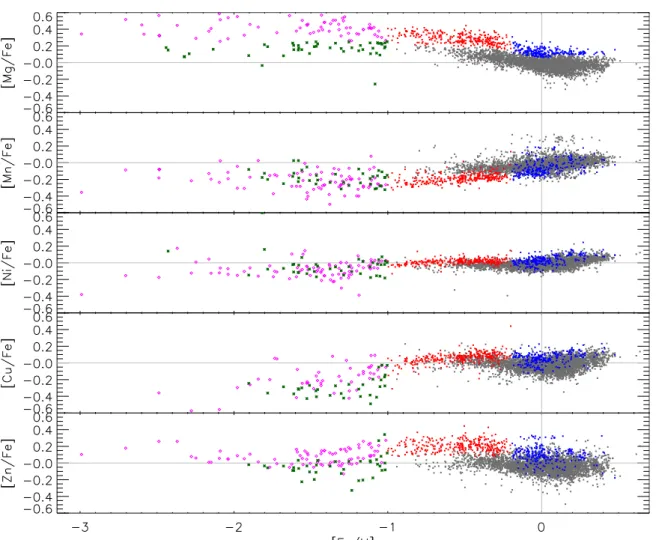
is one of the best α elements to define the Galactic disc com-ponents. We therefore adopt the same procedure in the present study, and the top panel of Fig.6shows the [Mg/Fe] distribution as a function of [Fe/H] for our final sample with a specific colour code for the different Galactic components defined below. This definition is based on [Mg/Fe] distributions in various metallic-ity bins, where the sample stars are tagged as thin (α-rich) or thick (α-poor) disc members.

As expected, the stars with [Fe/H] > –1.0 dex clearly sep-arate into two distinct α-poor and α-rich (thin and thick disc) populations. One can also see that the thick disc population has a gap in metallicity at about [Fe/H] ≈ –0.2 dex. This gap lies at the same location as inAdibekyan et al.(2011,2012), who used it to define the thick disc and α-rich metal-rich sequence. In the

following, we adopted this separation at [Fe/H] ≈ –0.2 dex to de-fine these two subpopulations of the disc.

As for the metal-poor stars ([Fe/H] < –1.0 dex), the top panel of Fig.6 shows that this subpopulation is also very well sepa-rated into α-rich and α-poor components. This trend was already observed byNissen & Schuster(2011). We identified the low-α and high-low-α metal-poor sequences using the same separation function as inNissen & Schuster(2010,2011) for metallicities in the range –1.6 dex to –1.0 dex. For [Fe/H] < –1.6 dex range, we adopted a separation criterium at [Mg/Fe] = 0.25 dex to de-fine the low- and high-α sequences. These authors have shown that low-α and high-α metal-poor sequences separate visually in the [Fe/H] versus [α/Fe] plane. They also have checked kine-matically, via a Toomre diagram, that the two sequences are dis-tinct. We point out that the metal-poor high-α group could con-tain both halo and thick disc stars because these populations are chemically indistinguishable (see e.g.Nissen & Schuster 2010). If these five Galactic components are mixed well, chemi-cally homogeneous, and well defined, one could expect that the scatter inside each component should be similar to the expected measurement errors. If not, either one of the component is not very well defined and/or the measurement errors are underes-timated; for example, some of the adopted atomic lines could be sensitive to NLTE effects. As a sanity check, we thus show a comparison between expected errors (red line) and measured dispersion (black line) in metallicity bins in the top panel of

Fig. 5.Effective temperature – surface gravity diagram of the main sam-ple stars. The metallicity is coded in colours in the upper panel and the assigned Galactic component is colour coded in the lower panel (tags

in the legend are the same as in Table5).

Fig.7. We require every metallicity bin to contain at least five stars. Otherwise the statistical result is not trustworthy, so it is not shown in the plot. That is why the metal-poor part of Fig.7

contains different number of data points for different elements. It can be seen that the observed dispersion around the trends is fully described by the expected errors, leaving little room for astrophysical dispersion. However, we point out that errors are overestimated in some metallicity bins. We indeed already no-ticed that the atmospheric parameters errors that we use are too pessimistic for many stars in our sample. We adopted the gen-eral typical errors (see footnote in Table2) provided by AMBRE (neglecting the co-variance and hence overestimating the errors) and summed than quadratically to compute the total error. For metal-poor stars, only the high-α sequence is shown because the low-α is too weakly populated.

Moreover, Fig. 7 indicates that the scatter in the thin and thick disc sequences is very low (≈0.05 dex). Actually, it pro-vides a very important observational constrain for Galactic evo-lutionary models that study the efficiency of the possible stellar radial migration. These models should satisfy the observed up-per limit of disup-persions for both discs.

In summary, we therefore defined five different compo-nents in our sample data: (1) the thin disc (α-poor) population that covers the metallicity range between [Fe/H] ≈ −0.8 dex

to [Fe/H] ≈ +0.5 dex and consists of 3949 stars (84.5% of the total sample); (2) the metal-rich high-α sequence from [Fe/H] ≈ –0.2 dex to [Fe/H] ≈ +0.3 dex (260 stars, 6% of the total sample); (3) the metal-poor (α-rich) thick disc that starts from [Fe/H] ≈ –1.0 dex and ends at [Fe/H] ≈ –0.2 dex (313 stars, 6.5% of the total sample). There are also 144 metal-poor ([Fe/H] < –1.0 dex) stars (3% of the total sample): (4) 49 of which are low-α stars, whereas (5) 95 of which are high-α stars. We have a rather similar population ratios between these five Galactic components as Adibekyan et al. (2012), but our final sample is more than four times larger. Every star from our final catalogue is tagged as a member of one of these five components in last column of Table5. The assigned Galactic components are colour coded in lower panel of effective temperature – surface gravity diagram (Fig.5).

4. Properties of the iron-peak elements in the different Galactic disc components

In this section, we present and discuss the iron-peak abundances for stars of our sample (4666 stars). We mostly focus on the disc components, although we further compare our results to other Galactic components. First we present the iron-peak chemical characterisation of the defined Galactic component (Figs.8and9

which show the mean tendencies), and then we discuss them in comparison with previous high-resolution spectroscopic studies devoted to the chemical properties of the Galactic disc.

4.1. Manganese

The only stable manganese isotope55_{Mn is produced by type-Ia}

and type-II supernovae in which thermonuclear explosive silicon burning and alpha-rich freeze-out via synthesis of55_{Co are}

ac-tive. They decay then via55Fe isotope to the stable55Mn (Truran et al. 1967). However, the yields from type-Ia supernovae are much larger (approximately by two orders of magnitude; see

Nomoto et al. 1997b,a;Kobayashi et al. 2006), so manganese is logically considered a characteristic yield of type-Ia supernovae (Seitenzahl et al. 2013).

In our sample stars, we observe an increasing trend of [Mn/Fe] with [Fe/H] (see Fig.6and8). Moreover, thin and thick disc populations are seen to follow the same trend with metal-licity. However, [Mn/Fe] abundances of thick disc stars tend to be smaller than thin disc stars by about 0.05 dex in the same metallicity range (Fig.8). More metal-rich high-α sequence stars could also be slightly less enriched in manganese than thin disc stars. Finally, the high-α and low-α metal-poor populations over-lap and do not have any distinguishable trends, although they seem to follow the thick disc trend forming a plateau around [Mn/Fe] = –0.25 dex.

The number of published observations of manganese is very large, but only three studies (Adibekyan et al. 2012;Battistini & Bensby 2015;Hawkins et al. 2015) report statistically represen-tative samples (1111, 714, 3200 stars, respectively). The man-ganese abundances of the thin and thick disc was first explicitly studied byFeltzing et al.(2007) who kinematically divided their sample of 95 dwarf stars into thin and thick disc components. Their thick disc sample is found to be lower in [Mn/Fe] than their thin disc stars by about 0.05 dex at the same metallicities, which agrees with our results based on a much more statisti-cally significant sample spanning a broader range of metallic-ity.Adibekyan et al. (2012) also clearly showed an increasing trend of [Mn/Fe] versus [Fe/H] for their sample of 1111 HARPS

Fig. 6.Observed element vs. iron abundance ratios as a function of the iron abundance. The different Galactic components defined in Sect.3

are plotted: thin disc (grey dots), thick disc (red dots), metal-rich high-α sequence (blue dots), metal-poor low-α sequence (green asterisk), and metal-poor high-α sequence (magenta rhombus); the light grey lines represent the solar values.

stars, which were chemically separated thin and thick disc sam-ples in a similar manner as in our study. They concluded that there are some hints indicating that the two discs have di ffer-ent [Mn/Fe] ratios, but there is no clear boundary between both discs. On the contrary and owing to our smaller dispersion, such a thin/thick disc dichotomy appears in a much clearer way in our sample, particularly for metallicities that are smaller than [Fe/H] ∼ −0.2 dex (see, for instance, Fig. 8). Furthermore, in their smaller sampleBattistini & Bensby (2015) found no sig-nificant distinction between thin and thick disc populations con-trary to what we clearly see. This could be because of a larger dispersion in their chemical analysis. However, NLTE correc-tions to their Mn abundances revealed a much clearer distinc-tion. Finally,Hawkins et al.(2015) reported high accuracy mea-surements of manganese abundance from the APOGEE survey for 3200 giant stars. They found different behaviours of man-ganese in the thin and thick discs: [Mn/Fe] abundance ratios in thin disc stars are generally larger than in thick disc stars. This is in good agreement with our results. For example, their thin and thick disc trends in [Fe/H] varying from –0.7 dex to –0.5 dex differ by 0.09–0.06 dex, which is very close to what we see in our data.

On the other hand, our metal-poor sample (144 stars) can be compared to the smaller samples of Reddy et al. (2006) and Reddy & Lambert (2008; 36 stars), Sobeck et al. (2006; 200 globular cluster stars),Nissen & Schuster(2011; 98 stars),

and Ishigaki et al. (2013; 78 stars). These investigations, in agreement with our results, observed an almost flat trend at [Mn/Fe] ∼ –0.3 dex from [Fe/H] ≈ –1.6 dex to –1.0 dex. We fi-nally point out thatNissen & Schuster(2011) andIshigaki et al.

(2013) also performed a chemical separation between high-α and low-α metal-poor stars. Similar to our results, based on a sample that was two times larger, they did not find any distinguishable [Mn/Fe] separation between the high-α and low-α metal-poor populations.

We have however several results for [Fe/H] < −2.5 dex that correspond to extremely metal-poor (EMP) stars. The num-ber of such stars is too small to have any statistics, but we can compare tendencies of our results with largest literature abun-dance sources of EMP stars; these sources are Cayrel et al.

(2004; 70 stars) andLai et al.(2008; 28 stars). The [Mn/Fe] be-haviours from both literature sources scatter by 0.3 dex around [Mn/Fe] ≈ –0.4 dex and our points are in agreement with these literature trends.

It is interesting to compare our results with other Galactic substructures, even if there is no bulge or any dwarf spheroidal galaxy (dSph) stars in our sample. Mn abundances of bulge gi-ants from Barbuy et al. (2013; 56 bulge giant stars) show a good agreement with our thin and thick disc stars for metallici-ties higher than [Fe/H] >≈ −0.7 dex, whereas, for lower abun-dances, the [Mn/Fe] values in the bulge appear to decrease faster than for the thick disc stars with [Fe/H] >≈ −0.7 dex. Similarly,

Metal-poor high-á Thin disc Thick disc Metal-rich high-á

Fig. 7.Mean expected errors (red line) and measured dispersion (black line) for the [El/Fe] ratios with respect to the metallicity (binned every

0.2 dex and 0.3 dex for the metal-rich and metal-poor samples, respectively) for the main Galactic components.

[Mn/Fe] abundances in dSphs are approximately at a similar level as our thin and thick disc stars (North et al. 2012;Jablonka et al. 2015;Romano et al. 2011;Sbordone et al. 2007). However, some of them show very specific trends that are opposite from what we see in the solar neighbourhood. For example, [Mn/Fe] in the dSph Sculptor galaxy (North et al. 2012) slowly de-creases from –0.2 to –0.5 dex with increasing metallicity (from −1.8 to –0.8 dex) and also ω Cen exhibits a decrease from –0.2 to −0.7 dex with increasing metallicity (from –1.8 to –0.8 dex). This very specific behaviour of [Mn/Fe] reveals that the chemi-cal enrichment history is different from that of Milky Way.

From the point of view of Galactic chemical evolution (GCE), it would be interesting to use reference elements other than iron because its nucleosynthesis channels are not uniquely coming both from explosive nucleosynthesis in type-II or type-I supernovae. A good choice would be oxygen (Cayrel et al. 2004) since it is the most abundant element after H and He and it comes from a single source. However, because of observational di fficul-ties, it would considerably degrade the accuracy of the derived trends. Another natural choice is magnesium, since its abun-dances are accurately determined and it is also mainly formed in massive supernovae (Shigeyama & Tsujimoto 1998). In the fol-lowing, we thus discuss our iron-peak abundances with respect to the Mg abundances (see Fig.9).

In our sample stars, we observe a global underabundance of [Mn/Mg] for the metal-poor stars. This [Mn/Mg] ratio then in-creases with [Mg/H] after type-I supernovae start to enrich the interstellar medium (ISM; see Fig. 9). This is expected since type-II supernovae produce significantly less manganese than magnesium (e.g. yields byKobayashi et al. 2006). We also point out that the [Mn/Mg] ratio in high-α metal-poor stars is much larger than in low-α metal-poor stars (by ≈–0.2 dex). However, this is probably caused by magnesium, since both metal-poor trends also differ by the same amount in the [Mn/Fe] versus [Mg/Fe] plot (see Fig.9, top panel). Moreover, the thin and thick disc trends are seen to be much more distinct in [Mn/Mg] (by ≈0.3 dex) than in [Mn/Fe] plane of Fig. 8. This manganese-magnesium behaviour suggests that the manganese enrichment history clearly has the opposite behaviour.

Actually, there are rather few studies in the literature devoted to the [Mn/α]-[α/H]. The only valuable sources for compari-son areBattistini & Bensby(2015), which is devoted to rather metal-rich stars, andHawkins et al.(2015).Battistini & Bensby

(2015) used another α element (titanium) as a reference element and showed fully separated [Mn/Ti]-[Ti/H] trends (by ≈0.2 dex) for the thin and thick discs.The [Mn/Ti] ratios for both discs are closer than the [Mn/Mg] discs probably because the yields of Ti from type-I supernovae are larger than those of Mg (e.g. yields byKobayashi et al. 2006). Nevertheless the trends ofBattistini & Bensby (2015) are in general agreement with our results.

Hawkins et al. (2015) suggested a new set of chemical abun-dance planes: [Mn/Mg], [α/Fe], [Al/Fe], and [C+N/Fe], which can help to disentangle Galactic components in a clean and e ffi-cient way independent of any kinematical data. From their Fig. 9, we actually see that the [Mn/Mg] ratio plays a key role in con-firming the thin and thick disc separation. Of course, that method should be studied in much more detail. However, we agree with

Hawkins et al.(2015) that the Mn-α ratio could be another good tool to chemically disentangle thin and thick disc stars.

In Fig. A.1, we show some interesting results about the [Fe, Ni, Cu, and Zn/Mn] trends with respect to [Mn/H]. The thick disc [Fe, Ni, Cu, and Zn/Mn] trends are generally found to be higher than the thin disc trends. The largest difference is found for [Zn/Mn] where the thin and thick discs differ by about ≈0.25 dex. In the metal-poor regime, the metal-poor trends of [Fe, Ni/Mn] overlap and are close to ≈0.20 dex. This is not the case for the [Cu, Zn/Mn] trends in the metal-poor regime for which the high-α sequence is found to be ≈0.20 dex larger than the low-α sequence.

4.2. Nickel

Nickel is also produced by silicon burning, but the [Ni/Fe] ra-tio in yields of type-Ia and type-II supernovae is similar (see

Nomoto et al. 2013). This leads to the characteristic flat [Ni/Fe] versus [Fe/H] behaviour shown in the second panel of Fig.6. The metal-poor stars are found in a plateau around [Ni/Fe] ≈ –0.1 dex with a small scatter. However, metal-poor trends are exactly

Fig. 8.Same plot as Fig.6, but data are averaged in [Fe/H] bins. Thin disc (thick grey solid line), thick disc (red solid line), metal-rich high-α sequence (blue dotted line), metal-poor low-α sequence (dash-dot green line), and metal-poor high-α sequence (dashed magenta line); the light

grey lines represent the solar values. The binning structure is the same as in Fig.7. The error bars represent the standard deviation associated with

the mean value.

equal between high-α and low-α stars. The thick disc popula-tion forms a plateau around [Ni/Fe] ≈ 0.0 dex with a very small scatter (σ = 0.04 dex). This plateau is also seen for the metal-rich high-α sequence with a soft increase of [Ni/Fe] at super-solar metallicities. The [Ni/Fe] distribution of the thin disc is very tight and steady around [Ni/Fe] ≈ 0.0 dex with a small in-crease in the supersolar metallicity regime as well. Generally thin and thick disc populations overlap with no strong evidence of any chemical separation, although thin disc stars could reveal a slightly smaller [Ni/Fe] ratio.

To date, the largest samples of observed [Ni/Fe] were stud-ied byBensby et al.(2014; 714 stars),Adibekyan et al.(2012; 1111 stars), and alsoHawkins et al.(2015; 3200 APOGEE gi-ant stars). Regardless the adopted method for the thin/thick disc separation (Bensby et al. 2014, kinematically;Adibekyan et al. 2012, chemically and kinematically;Hawkins et al. 2015, chem-ically), the chemical patterns of [Ni/Fe] for the thin and thick discs are rather similar to ours. The [Ni/Fe] plateau was also

observed for metal-poor stars (around ∼ –0.1 dex for [Fe/H] < −1.0 dex) byReddy et al.(2006),Reddy & Lambert(2008) and it agrees with our results.Nissen & Schuster(2010) found that the high-α sequence is tight and follows the solar Ni value whereas the low-α sequence has a lower [Ni/Fe] ratio by –0.15−–0.1 dex. However, this finding is not confirmed in a similar study by

Ishigaki et al. (2013) who did not report any different nickel trends between their high-α and low-α samples. Our results sup-port the conclusion ofIshigaki et al.(2013).

[Ni/Fe] results of EMP stars byCayrel et al.(2004; 70 stars) and Lai et al. (2008; 28 stars) scatter by 0.25 dex around [Mn/Fe] ≈ –0.1 dex. That is in general agreement with our results.

The Ni abundances in the bulge fromJohnson et al.(2014; 156 giant stars) show a similar trend as our thin and thick disc stars, although they seem to be richer by ≈0.1 dex in the bulge. Such a small difference could be caused by small systematic offset.

Fig. 9.Same plot as Fig.8, but for the [X/Mg] vs. [Mg/H] ratios. The binning structure is the same as in Figs.7and8. The error bars represent the standard deviation associated with the mean value.

On the other hand, we point out that the trend of [Ni/Mg] with respect to [Mg/H] (Fig.9) is very similar to the [Fe/Mg] trend, confirming that nickel and iron are produced in similar supernovae environments.

We used nickel as a reference element in Fig.A.2. Obviously, since nickel and iron are very close in behaviour, all [Mn, Fe, Cu, and Zn/Ni] ratios with respect to [Ni/H] show very similar trends as was the case for [El/Fe] versus [Fe/H] in Fig.8.

4.3. Copper

Copper is an intermediate element between the iron-peak and the neutron capture elements, thus its nucleosynthesis is very complex. For instance, Bisterzo et al. (2004) highlighted sev-eral possible nucleosynthesis scenarios of the Cu origin: (i) ex-plosive nucleosynthesis during type-Ia; (ii) type-II supernovae explosions; (iii) weak s process occurring during He-burning in massive stars; (iv) main s process during helium burning in low-mass AGB stars; and also (v) weak sr process. First,McWilliam & Smecker-Hane (2005), based on a comparison of Cu in our

Galaxy and the Sgr dwarf spheroidal galaxy, showed that the type-Ia supernovae yields of Cu could be negligible and the type-II supernovae contribution of Cu could be up to 5%. Thus neutron capture processes are significant contributors of copper in the Galaxy (Bisterzo et al. 2004). The Cu contribution of s processes in the solar system is indeed around 27% (Bisterzo et al. 2004) coming from AGB and massive stars. However AGB stars could contribute only marginaly (5% contribution) since Bisterzo et al. claim that the bulk of cosmic Cu has actu-ally been produced by the weak sr process.

The Cu abundances derived for our sample stars (see Figs.6

and 8) show that each Galactic component has a specific be-haviour in the [Cu/Fe] versus [Fe/H] plane. First, the thick disc stars look slightly more enriched in Cu than thin disc stars by about 0.05 dex. The thin disc sample varies around [Cu/Fe] ≈ 0.0 dex with a small positive slope in the superso-lar metallicity regime. Both discs also show a mild increase in [Cu/Fe] at supersolar metallicities up to [Cu/Fe] ≈ 0.1 dex. On the other hand, the metal-poor stars ([Fe/H] < −1.0) show a larger scatter and an increase of [Cu/Fe] towards higher

metallicities from [Cu/Fe] ≈ –0.5 at [Fe/H] ≈ –2.0 to solar at [Fe/H] ≈ –1.0, reaching the level of the thick disc stars. High-and low-α sequences partially overlap but low-α stars are found to have a smaller [Cu/Fe] than the high-α stars by about 0.2 dex. There are no published observations of very large samples of stellar copper abundances. Homogoenous samples were anal-ysed byReddy & Lambert (2008; 60 metal-poor stars),Reddy et al. (2003; 181 metal-rich stars), Yan et al. (2015; 64 late type stars), and Mishenina et al. (2011; 172 metal-rich stars). The largest non-uniform sample was collected byBisterzo et al.

(2006; more than 300 stars) from various literature sources. Generally, our results agrees with Reddy & Lambert (2008), where they showed a tight distribution and mild positive trend of a kinematically defined thick disc (up to [Fe/H] = –0.25 dex) sample. Also, similar to our results, the thin and thick disc distri-butions ofMishenina et al.(2011),Reddy et al.(2003), andYan et al.(2015) are generally mixed and scattered, but with a mild thick disc overabundance comparing to thin discs. The overall picture of the sample collected by Bisterzo et al. (2006) from various sources is also in agreement with our observation. Thin disc stars (Bisterzo et al. 2006, sample) are obviously [Cu/Fe] poorer than thick disc stars at the same metallicities; thick disc stars show a distinguishable trend and mild [Cu/Fe] increase up to [Fe/H] = –0.4 dex.

For the metal-poor stars, Reddy et al. (2006), Reddy & Lambert(2008),Nissen & Schuster(2011),Ishigaki et al.(2013) observed scattered [Cu/Fe] abundances with a positive slope from [Cu/Fe] ≈ –0.5 dex up to solar [Cu/Fe] at [Fe/H] ≈ –1.0 dex. This agrees very well with our results. Furthermore, Nissen & Schuster(2011) showed that low-α metal-poor stars have signif-icantly lower [Cu/Fe] than high-α stars. This was later confirmed by Ishigaki et al. (2013). Cu from Nissen & Schuster (2011) was also reanalysed in LTE and NLTE byYan et al.(2016) who showed that even if there are some differences in the LTE/NLTE abundances, the general behaviour is not changed. Our study strengthens these results.

Finally, [Cu/Fe] abundance ratios in EMP stars byLai et al.

(2008; 28 stars) show a tendency to decrease with decreasing metallicity. Our results for the most metal-poor stars show the same tendency.

We also point out that the [Cu/Fe] abundances in the bulge fromJohnson et al.(2014; 156 giant stars) generally overlap that of the thin and thick discs. However these abundances scatter a lot (by ≈0.4 dex). Moreover, these abundance trends extend up to [Cu/Fe] ≈ 0.8 dex at [Fe/H] ≈ 0.5 dex.

Finally, the trend of [Cu/Mg] with respect to Mg (see Fig.9) is actually similar to those of [Fe/Mg] or [Ni/Mg]. As for these iron-peak species, the division between thin and thick discs are weak but real. The [Cu/Mg] ratio is found to stay constant and null for almost all thin discs, suggesting that the enrichment by supernovae of type-I did not produce any large amounts of copper.

In Fig. A.3, we adopted copper as a reference element to study the [Mn, Fe, Ni, and Zn/Ni] trends. This figure shows that the evolution of copper, nickel. and ion are actually very similar in the [Cu/H] > −1.0 dex regime. All these three sequences indeed overlap and are close to [El/Cu] ≈ 0.0 dex. Moreover, whereas [Mn/Cu] and [Zn/Cu] show the exact opposite be-haviour, the [Mn/Cu] thick disc trend is noticeably lower than the thin disc trend and the [Zn/Cu] thick disc trend is higher than in the thin disc. Finally, the picture in the metal-poor regime is rather different. Every [Mn, Fe, Ni, and Zn/Ni] high-α and low-α sequences behave similarly, i.e. [El/Cu] increases with decreas-ing of [Cu/H].

4.4. Zinc

Zinc, as copper, is an intermediate element between the iron-peak and the neutron capture elements. It is produced by the same nucleosynthesis channels but with different contribution ratios. Up to half of the zinc is indeed spread out by type-II su-pernovae or hysu-pernovae via64_{Zn, which is produced from α-rich}

freeze-out in γ winds. The remaining part (66,67,68,70_{Zn) is}

pro-duced by the sr process in massive stars (Bisterzo et al. 2004). Type-Ia supernovae and s process occurring in AGB stars pro-duce only a marginal part of zinc nuclei.

Our study reveals that the [Zn/Fe] versus [Fe/H] distribution of thick and thin disc stars show specific and distinct behaviours (see Figs.6 and8). The entire thick disc is obviously [Zn/Fe] richer than the thin disc. Moreover, the metal-poor part of the thick disc distribution is (red points) is tight and clearly sepa-rates from the thin disc at the same metallicities by about 0.2 dex whereas the thin disc [Zn/Fe] distribution is constant around the solar value, regardless of the metallicity. These thin and thick disc distributions of [Zn/Fe] are very similar to the [α/Fe] distri-butions (see top panel of Fig.6). We therefore propose that zinc could be a very good species to chemically disentangle the thin and thick disc components in the Galaxy.

The main α-like behaviour of zinc in the discs was already marginally mentioned in some previous studies, which anal-ysed uniform, but smaller samples (see, for instance the results of 172 FGK stars by Mishenina et al. 2011 or 714 stars by

Bensby et al. 2014) and also non-uniform data collections as in

Bisterzo et al.(2006; 380 stars) andSaito et al.(2009; 434 stars).

Barbuy et al.(2015) showed that [Zn/Fe] in bulge stars also con-firms its α-like behaviour. However, the very clear separation between the thin and thick discs was never demonstrated before. On the other hand, the trend of [Zn/Fe] for the metal-poor α-rich stars is close to the solar value up to [Fe/H] ≈ –1.3 and then becomes slightly positive up to [Fe/H] ≈ –1.0 dex, where it reaches supersolar [Zn/Fe] values and smoothly connects to the thick disc. The low-α sequence is generally lower than the high-α sequence (by ≈0.15 dex). The largest uniform sample that can be used for comparison is that ofIshigaki et al.(2013; 97 stars), which showed very similar results that are also seen in the non-uniform samples ofBisterzo et al.(2004) andSaito et al.(2009). Finally,Nissen & Schuster(2011) also found that low-α metal-poor stars have significantly lower [Zn/Fe] ratios than high-α stars in their analyses. This tendency was confirmed byIshigaki et al.(2013) and, again, agrees with our results based on a much larger and confident sample. According toNissen & Schuster

(2011), NLTE corrections would lead to systematic changes in the derived [Zn/Fe] values by less than than ±0.1 dex. This con-clusion is based on the work ofTakeda et al.(2005) who esti-mated the NLTE corrections for the three zinc lines selected for our analysis. Indeed, most of the NLTE-LTE abundance di ffer-ences do not exceed 0.1 dex for the 4722 and 4810 Å lines. These differences are mostly used to derive abundances for metal-poor stars, as shown byTakeda et al.(2005), whereas the 6362 Å line, mostly used in the [Fe/H] > –1.0 dex regime, is even less affected by such differences. According toTakeda et al.(2005,2016), we thus do not expect Zn NLTE-LTE corrections to be larger than 0.03 dex and 0.06 dex for dwarfs and giants, respectively.

The [Zn/Fe] abundances of EMP stars byCayrel et al.(2004; 70 stars) andLai et al.(2008; 28 stars) show a clear tendency to increase with decreasing metallicity from [Zn/Fe] ≈ 0.15 dex at [Fe/H] ≈ –2.5 dex to [Zn/Fe] ≈ 0.50 dex at [Fe/H] ≈ –3.5 dex, although with a scatter as large as 0.25 dex. Our [Zn/Fe] results