HAL Id: hal-03084224
https://hal.archives-ouvertes.fr/hal-03084224
Submitted on 30 Dec 2020
HAL is a multi-disciplinary open access
archive for the deposit and dissemination of
sci-entific research documents, whether they are
pub-lished or not. The documents may come from
teaching and research institutions in France or
abroad, or from public or private research centers.
L’archive ouverte pluridisciplinaire HAL, est
destinée au dépôt et à la diffusion de documents
scientifiques de niveau recherche, publiés ou non,
émanant des établissements d’enseignement et de
recherche français ou étrangers, des laboratoires
publics ou privés.
Distributed under a Creative Commons Attribution - NoDerivatives| 4.0 International
License
Spatial and Temporal Variability of the North Atlantic
Eddy Field From Two Kilometric-Resolution Ocean
Models
Adekunle Ajayi, Julien Le Sommer, Eric Chassignet, Jean-marc Molines,
Xiaobiao Xu, Aurelie Albert, Emmanuel Cosme
To cite this version:
Adekunle Ajayi, Julien Le Sommer, Eric Chassignet, Jean-marc Molines, Xiaobiao Xu, et al..
Spa-tial and Temporal Variability of the North Atlantic Eddy Field From Two Kilometric-Resolution
Ocean Models.
Journal of Geophysical Research.
Oceans, Wiley-Blackwell, 2020, 125 (5),
Ocean Models
Adekunle Ajayi1 , Julien Le Sommer1 , Eric Chassignet2 , Jean-Marc Molines1,
Xiaobiao Xu2 , Aurelie Albert1 , and Emmanuel Cosme1
1Universite Grenoble Alpes /CNRS/IGE, Grenoble, France,2Florida State University, Tallahassee, FL, USA
Abstract
Ocean circulation is dominated by turbulent geostrophic eddy fields with typical scales ranging from 10 to 300 km. At mesoscales (>50 km), the size of eddy structures varies regionally following the Rossby radius of deformation. The variability of the scale of smaller eddies is not well known due to the limitations in existing numerical simulations and satellite capability. Nevertheless, it is well established that oceanic flows (<50 km) generally exhibit strong seasonality. In this study, we present a basin-scale analysis of coherent structures down to 10 km in the North Atlantic Ocean using twosubmesoscale-permitting ocean models, a NEMO-based North Atlantic simulation with a horizontal resolution of 1/60 (NATL60) and an HYCOM-based Atlantic simulation with a horizontal resolution of 1/50 (HYCOM50). We investigate the spatial and temporal variability of the scale of eddy structures with a particular focus on eddies with scales of 10 to 100 km, and examine the impact of the seasonality of submesoscale energy on the seasonality and distribution of coherent structures in the North Atlantic. Our results show an overall good agreement between the two models in terms of surface wave number spectra and seasonal variability. The key findings of the paper are that (i) the mean size of ocean eddies show strong seasonality; (ii) this seasonality is associated with an increased population of submesoscale eddies (10–50 km) in winter; and (iii) the net release of available potential energy associated with mixed layer instability is responsible for the emergence of the increased population of submesoscale eddies in wintertime.
Plain Language Summary
The ocean is dominated by circular currents of water in swirling motion called oceanic eddies. This class of motion is by far the largest reservoir of oceanic kinetic energy. Much is known about this oceanic eddies at scale>50 km while we are yet to fully comprehend their distribution in terms of size and dynamics at scales<50 km. This is due to the lack of sufficientobservational data sets at these scales in the ocean. In this study, we use two kilometric-resolving models of the North Atlantic ocean to investigate the spatial and temporal variability of oceanic eddies down to 10-km scale. Our results show that the distribution of oceanic eddies at spatial scale<100 km undergo strong seasonality and that this seasonality is as a result of an increased population of smaller eddies (10–50 km) often called submesoscales eddies in wintertime. We found that submesoscale turbulence (a class of oceanic turbulence at fine scale) is responsible for the increase in smaller-scale eddy distribution in winter.
1. Introduction
Ocean circulation combines large (>500 km), meso (50–500 km) and submesoscale (1–50 km) structures that result from direct forcing and energy exchanges through nonlinear scale interactions. The ocean is a turbulent fluid, and most of its energy is concentrated in geostrophically balanced eddy fields. The coher-ent structures that make up the eddy field are mostly generated by baroclinic instability in an intensified ocean flow (Stammer, 1997) and therefore scale with the first Rossby radius of deformation. These ubiqui-tous, energetic, time-dependent circulations have their signature in all aspects of ocean activities and have, therefore, been defined as the weather system of the ocean (Bryan, 2008; McWilliams, 2016).
Improving our knowledge of the scale of eddy structures is key to several applications in physical oceanog-raphy. The interaction between the eddy field and large-scale flow is one of the main drivers of ocean circulation. This interaction is presently parameterized in noneddy-resolving ocean and climate models, and
Key Points:
• The scale of North Atlantic eddies with scale<100 km is studied using two kilometric-resolution ocean models
• The mean size of these eddies varies across the basin and shows a strong seasonality
• This seasonality is driven by mixed layer instability and is associated with an increased population of submesoscale eddies in winter
Correspondence to:
A. Ajayi,
adekunle.ajayi@univ-grenoble-alpes.fr
Citation:
Ajayi, A., Le Sommer, J., Chassignet, E., Molines, J.-M., Xu, X., Albert, A. & Cosme, E. (2020). Spatial and temporal variability of the North Atlantic eddy field from two kilometric-resolution ocean models. Journal of Geophysical
Research: Oceans, 125, e2019JC015827. https://doi.org/10.1029/2019JC015827
Received 30 OCT 2019 Accepted 14 APR 2020
Accepted article online 20 APR 2020
©2020. The Authors.
This is an open access article under the terms of the Creative Commons Attribution License, which permits use, distribution and reproduction in any medium, provided the original work is properly cited.
Journal of Geophysical Research: Oceans
10.1029/2019JC015827
the parameterizations used in these models are usually derived from a mixing length hypothesis based on eddy velocity and eddy length scale to derive eddy diffusivity (Bates et al., 2014; Fox-Kemper et al., 2008). The correlation scale of mesoscale eddies is also central to the design of the inversion algorithm used in satellite remote sensing. For instance, the optimal interpolation method currently used in calibrating AVISO prod-ucts takes as input correlation radii based on eddy length scales (Amores et al., 2019; Ducet & Traon, 2001). If the typical scale of eddies varies in time and space in the ocean, then this variability should be accounted for in ocean model parameterizations schemes and satellite data interpolation algorithms, hence the need to document how the scale of eddy vary in space and time.Satellite missions have revolutionized the way we see the Earth surface from space and continue to serve as a large-scale observational platform for modern oceanography. Satellite data are currently the primary source of knowledge about oceanic eddies, their scales, and their variability. A concise review of the knowledge gained from using satellite altimeters to study mesoscale eddies in the global ocean is presented in Fu et al. (2010). Early works include a regional study on the variability of mesoscale eddies using Geosat by Le Traon et al. (1990), where the authors inferred scales of eddies from the spatial autocorrelation function of observed sea surface height (SSH) fields and recorded a high variability of mesoscale eddy fields in space across the entire North Atlantic. More recently, the merging of altimeter products covering a 16-year period paved the way for the automated identification, tracking, and documentation of about 35,000 mesoscale eddies with a lifetime greater than 16 weeks (Chelton et al., 2011). This analysis confirmed that the observed eddy scales mostly fall between the first Rossby radius of deformation Ldand the Rhines scale Ld(Klocker & Abernathey, 2014). This is in agreement with Eden (2007) who found in an eddy-permitting numerical simulation of the North Atlantic that north of 30◦N eddy scales are isotropic and proportional to Ld, while south of 30◦N the eddies' scales are more closely related to the Lr. The scale min(Lr,Ld) was found to be the best predictor of eddy scale over the entire North Atlantic domain.
Studies focusing on coherent eddy structures in the ocean have mostly been limited to structures with scales on the order of 100 km (Amores et al., 2018). This is mainly due to the nonavailability of a high-resolution global oceanic data set for the smaller wavelength range, a consequence of the limitations of existing numerical and satellite altimetry capability (Dufau et al., 2016). That being said, several ocean models, such as the NEMO-based North Atlantic simulation with a horizontal resolution of 1/60◦(NATL60) and the HYCOM-based Atlantic simulation with a horizontal resolution of 1/50◦(HYCOM50), were designed in preparation for the upcoming Surface Water and Ocean Topography (SWOT) altimeter mission (Fu & Ubelmann, 2014). These simulations now have the ability to capture explicitly ocean circulation at the basin scale down to 10 km and therefore provide a platform to investigate the variability of eddy structures at scales less than 100 km.
At scales smaller than 100 km, oceanic flows are dominated by surface-intensified energetic submesoscale motions, and they include coherent vortices, fronts, and filaments. Furthermore, both observations and model simulations have shown that submesoscale motions undergo a strong seasonality with large ampli-tudes in winter (Brannigan et al., 2015, 2015 Callies, Ferrari, Klymak, et al., 2015; Qiu et al., 2014; Rocha et al., 2016; Sasaki et al., 2014). The emergence in winter of submesoscale motions has been attributed to frontogenesis, wind-induced frontal instabilities, and mixed layer instability (McWilliams, 2016; Thomas, 2013). Mixed layer instability (which is associated with the weakening of surface stratification in winter conditions) has been put forward as the dominant mechanism driving the emergence of submesoscales in winter in midlatitudes (Callies, Flierl, Ferrari, et al., 2015; Capet et al., 2008; Mensa et al., 2013; Qiu et al., 2014 Sasaki et al., 2014).
In this paper, the emphasis is on eddies with scales<100 km, with a focus on coherent structures within the 10–50 km-scale range, hereafter referred to as submesoscale eddies (SMEs) (Sasaki et al., 2017). Our key objective is to investigate how resolving submesoscales affects eddy motions and their variability, specifically in terms of spatial scale and depth penetration. This paper intends to answer this question by documenting the statistics of SMEs and their overall impact on the variability of mean eddy scales in the North Atlantic. This is done by first performing a basin-scale analysis of the spatial and temporal variability of coherent structures down to 10 km in the North Atlantic Ocean using two submesoscale resolving ocean models, NATL60 and HYCOM50. Then, we examine the impact of the seasonality of submesoscale energy on the distribution and depth penetration of eddy structures in the North Atlantic. The result of this study (to name a few) would contribute to (i) improve eddy parameterization scheme used in noneddying ocean models and
(ii) inform satellite data interpolation algorithms by taking into account the temporal and spatial variability of eddy scales.
This paper is organized as follows: In section 2, we provide a description of the NATL60 and HYCOM50 data sets. In sections 3 and 4, we present the temporal and spatial variability of eddy scales, respectively. Section 5 presents the impact of the seasonality of submesoscale energy on eddy scale variability. We summarize and conclude our analysis in section 6.
2. Data Sets and Methodology
2.1. North Atlantic Ocean Model Simulations
In this study, we use numerical outputs from two submesoscale eddy-permitting simulations of the North Atlantic: a NEMO-based North Atlantic simulation with a horizontal resolution of 1/60◦(NATL60) and a HYCOM-based Atlantic simulation with a horizontal resolution of 1/50◦(HYCOM50).
The NEMO-based NATL60 has a horizontal grid spacing that ranges from 1.6 km at 26◦N to 0.9 km at 65◦N. The grid has been designed so that the model explicitly simulates the scales of motions that will be observed by the SWOT altimetric mission. In practice, the model's effective resolution is about 10–15 km in wavelength. The initial and open boundary conditions are based on GLORYS2v3 ocean reanalysis with a relaxation zone at the northern boundary for sea ice concentration and thickness. The model has 300 verti-cal levels with a resolution of 1 m at the topmost layers. The atmospheric forcing is based on DFS5.2 (Dussin et al., 2018). The grid and bathymetry follow Ducousso et al. (2017). In order to implicitly adapt lateral vis-cosity and diffusivity to flow properties, a third-order upwind advection scheme is used for both momentum and tracers in the model simulation. The model is spun-up for a period of 6 months, and a 1-year simulation output from 2012 to 2013 is used in this study. The outputs of this simulation have also been used in recent studies (Amores et al., 2018; Buckingham et al., 2019).
The HYCOM-based HYCOM50 extends from 28◦S to 80◦N and has a horizontal grid spacing ranging from 2.25 km at the equator, ∼1.5 km in the Gulf Stream region, and 1 km in the subpolar gyre. As for NATL60, the effective resolution is about 10–15 km. The vertical coordinate is hybrid and consists of 32 layers. The simulation is initialized using potential temperature and salinity from the GDEM climatology and spun up from the rest for 20 years using climatological atmospheric forcing from ERA-40 (Uppala et al., 2005), with 3-hourly wind anomalies from the Fleet Numerical Meteorology and Oceanography Center 3-hourly Navy Operational Global Atmospheric Prediction System (NOGAPS) for the year 2003. The last year of the simu-lation is used to perform the analysis. The horizontal viscosity operator is a combination of Laplacian and Biharmonic. The bathymetry is based on the Naval Research Laboratory (NRL) digital bathymetry database. The model configuration and a detailed evaluation of the model results in the Gulf Stream region with observations are documented in Chassignet and Xu (2017).
Both NATL60 and HYCOM50 resolve the first Rossby radius of deformation everywhere within the model domains, and these simulations reproduce realistic eddy statistics with levels of kinetic energy in the range of altimetric observations (Figure 1). HYCOM50 shows a higher eddy kinetic energy (EKE) level along and around the Gulf Stream-North Atlantic Current path. The less energetic Gulf Stream-North Atlantic Current in the NATL60 simulation may be due, in part, to its shorter spin-up period (6 months versus 19 years). A summary of the model parameters is tabulated in Table 1. In this study, we consider the outputs of HYCOM50 for exactly the same region covered by NATL60 to have comparable results, and we perform statistical anal-ysis of the model outputs in two-dimensional 10◦×10◦boxes, following earlier approaches by Stammer and Böning (1992), Uchida et al. (2017), and Chassignet and Xu (2017).
2.2. Wave Number Spectra
Wave number spectra provide a way to quantify the variability and energy associated with motions of dif-ferent spatial scales across difdif-ferent regions. In this study, spectral analysis is performed in subdomains of 10◦×10◦boxes across the North Atlantic in order to document regional variability. Prior to spectral analy-sis, the field of each box is detrended in both directions, and a 50% cosine taper window (turkey windowing) is applied for tapering. a fast Fourrier transform (FFT) is applied to the tapered data, and a one-dimensional isotropic spectrum is obtained by averaging over all azimuthal directions. Our spectral approach is in line with Chassignet and Xu (2017), and because we are making use of year 20 of the HYCOM50 simulation used in Chassignet and Xu (2017), we were able to compare our SSH wave number spectra estimates with the already published results for the same data set and found our result to be consistent as well (not shown).
Journal of Geophysical Research: Oceans
10.1029/2019JC015827
Figure 1. Surface eddy kinetic energy (cm2s−2) computed from daily mean outputs of the total velocity. (a) NATL60 and (b) HYCOM50.
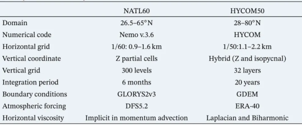
Figure 2 shows the wave number power spectral density for SSH, surface kinetic energy (KE), and surface relative vorticity (RV) in a region close to the Gulf Stream (Box 1, as defined in Figure 1) for the two data sets. The wave number power spectra from the two models agree well, indicating that the distribution of energy across scales is similar in both models. The estimated slope from the SSH and KE spectra indicates that the two models agree with quasigeostrophic dynamics, which predict a slope of k−5and k−3for SSH and KE spectra, respectively. This agreement is particularly strong for the wavelength band of 10–100 km. HYCOM50 shows more variance at low wave numbers compared to NATL60. This is consistent with the lower EKE in NATL60 compared to HYCOM50 at these scales (Figure 1). In Figure 3, we present the seasonality of SSH, KE, and RV wave number power spectral density. At scales smaller than 100 km, the variance of SSH, KE, and RV is of higher magnitude in winter (January, February, and March) compared to summer (July, August, and September). Whereas, the variance associated with scales larger than 100 km has a higher magnitude in
Table 1
Table of Model Parameters for NATL60 and HYCOM50
NATL60 HYCOM50
Domain 26.5–65◦N 28–80◦N
Numerical code Nemo v.3.6 HYCOM
Horizontal grid 1/60: 0.9–1.6 km 1/50:1.1–2.2 km
Vertical coordinate Z partial cells Hybrid (Z and isopycnal)
Vertical grid 300 levels 32 layers
Integration period 6 months 20 years
Boundary conditions GLORYS2v3 GDEM
Atmospheric forcing DFS5.2 ERA-40
Figure 2. One year average wave number power spectra density in a 2-D 10◦square box (Box 1, Figure 1) around the energetic Gulf Stream region computed from daily output of NATL60 (thick black line) and HYCOM50 (thick dash line). (a) SSH, (b) surface KE from total velocity, and (c) surface relative vorticity.
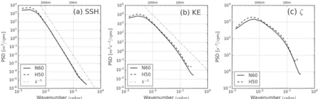
the summer compared to winter. This winter-to-summer contrast is more pronounced in RV wave number spectra and is usually more visible in a winter-summer contrast of an RV snapshot (Figure 4).
The overall assessment shows that NATL60 and HYCOM50 agree reasonably well with each other on the dynamics governing the ocean surface. The small mismatch between the result of the models may be a function of the differences in the model parameters and the length of their spin-up. In the next section, we focus on describing the statistics of eddy scales, as seen in the two simulations.
2.3. Eddy Length Scale Metric
A well-known approach for describing turbulent oceanic flows is to identify the typical length scale of motion that characterizes the dynamics of the flow. This involves computing the integral length scale of the energy-containing eddies (Moum, 1996; Qiu et al., 2014) or the enstrophy-containing scale (Morris & Foss, 2005; Scott, 2001) from the velocity and vorticity wave number spectrum, respectively. These length scales in physical space correspond to the scale of the most energetic eddy structures and are roughly consistent with the mean scale of eddies that can be identified by eddy detection algorithms (Chelton et al., 2007, 2011; Stammer, 1997).
In this paper, we measure mean eddy scales in each of our study regions by estimating the enstrophy-containing scale L𝜁from the vorticity wave number power spectra density following Scott (2001).
Figure 3. Winter (January-February-March) (thick black line) and summer (July-August-September) (thick dash line)
wave number power spectra density in a 2-D 10◦square box (Box 1, Figure 1) around the energetic Gulf Stream region
Journal of Geophysical Research: Oceans
10.1029/2019JC015827
Figure 4. Seasonality of resolved vorticity field in (a, b) NATL60 and (c, d) HYCOM50 in Box 1.
The vorticity wave number spectral density is estimated (as described in section 2.2) using surface rel-ative vorticity computed from the daily averaged model outputs. The enstrophy-containing scale is the enstrophy-weighted mean scale defined in equation (1), and it represents the scale of the most intense vor-tical structure in that flow. In equation (1), Z(k, l) denotes the vorticity wave number power spectral density, while k and l are the zonal and meridional wave number, respectively.
L𝜁 = ∫ ∫ Z(k, l)dkdl
∫ ∫ √k2+l2Z(k, l)dkdl (1)
To describe the distribution of the individual coherent eddy structures, we used an automated eddy detection algorithm. The algorithm detects coherent eddies by identifying closed SSH contours. A closed contour is then identified as an eddy if it satisfies some specific criteria with regard to its amplitude, number of pixels, the existence of at least one local extremum, and so forth. The successful application of the algorithm is documented in Chelton et al. (2011). This method is hereafter referred to as C11, and the corresponding eddy scale is referred to as L𝜂. We applied C11 to daily averages of SSH in two-dimensional 10◦boxes for a period of 1 year. The implementation of the C11 algorithm in Python is available online at this site (https:// github.com/chrisb13/eddyTracking).
3. Temporal Variability of Eddy Scale
In this section, we present the temporal variability of eddy statistics across the North Atlantic. The analysis is presented for both winter (January, February, and March) and summer (July, August, and September) in two regions: the Gulf Stream extension (Box 1 (Boxes already defined in Figure 1.)) and the Labrador sea (Box 11). These two boxes were selected because Box 1 is a well-documented high-EKE region (Mensa et al., 2013) while Box 11 (a relatively low EKE region compared to Box 1) is a region with a very deep mixed layer in winter and energetic submesoscale activities.
In Figure 5, we present the vorticity wave number spectra for winter and summer in Box 1 and Box 11. In both boxes, vorticity wave number spectra vary notably from winter to summer, with the peak and the estimated
Figure 5. Surface relative vorticity wave number spectra for Box 1 and Box 11 (box defined in Figure 1), calculated from daily averages for winter time, JFM (red line) and summer time, JAS (blue line). Thick dots represent
enstrophy-containing scale (L𝜂) for each spectra. (a) NATL60 Box 1, (b) HYCOM50 Box 1, (c) NATL60 Box 11,
and (d) HYCOM50 Box 11.
enstrophy-containing scale, L𝜁(thick dots) of the spectra shifting to finer scales in winter. This change is evident in both models and in both regions. This seasonality is made more obvious in the 1-year time series of L𝜁 for Box 1 (Figure 6). The winter and summer mean of the enstropy-containing scale presented in Figure 7 show that this seasonality is pronounced everywhere in the North Atlantic. The mean of L𝜁is about a factor of 2 larger in summer compared to winter. Similarly, the magnitude of the enstrophy-containing scale and spectra density vary from one region to another. The enstrophy-containing scale in Box 1 is of higher wavelength compared to that in Box 11. This type of regional difference in the spectra estimates and its weighted scale represents the spatial variability associated with the energy of the vortical structures across
Figure 6. Time series of the enstrophy-containing scale L𝜁for Box 1 (NATL60 data set). The enstrophy-containing scale is the enstrophy-weighted mean scale defined in equation (1). The dashed vertical lines represent the beginning and end of the seasons.
Journal of Geophysical Research: Oceans
10.1029/2019JC015827
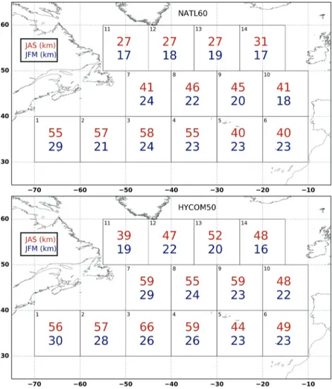
Figure 7. Map of mean eddy length scale (L𝜁) in winter (JFM) and summer (JAS) for (a) NATL60 and (b) HYCOM50.
the North Atlantic. We are going to discuss this further in section 4. Regardless of the model or region, the winter spectra compared to the summer spectra show higher variance at high wave numbers (Figure 5). This indicates that smaller-scale structures (>70 km) are more energetic in winter compared to summer. In order to explain the seasonality of the enstrophy-containing scale in terms of the statistics of isolated eddy structures, Figure 8 shows the distribution of eddy scales obtained from the application of C11 to SSH fields. The histogram shows eddies with a lifetime greater than 10 days, in order to filter out short-lived features wrongly identified as eddies by the algorithm. In the plot, the seasonal differences in the distributions of the scales of eddies are more pronounced for eddies with scales smaller than 50 km. Following our definition of submesoscales eddies (SMEs) as eddies with scales from 10 to 50 km, we find that the seasonality of enstrophy-containing scale is attributed to an increased population of SMEs in winter. This information is supported by our analysis for both models across the North Atlantic and is, therefore, a robust signal. The increase in the number of detected SMEs in winter corroborates the large variance at high wave num-bers in the vorticity spectra and also explains the reduction in the mean scale of eddies from summer to winter. However, we should note that the information about SME seasonality from the application of C11 highlights only the coherent structures, while the results of the spectra at a high wave number might include the vorticity variance coming from fronts, filaments, and all other active submesoscales features other than coherent vortices. Noticeable in Figure 8 is the discrepancy in the tails of eddy scale distribution. In particu-lar, there are more large-scale eddies (>50 km) in HYCOM50 compare to NATL60. This difference, observed in most of the boxes, maybe due to the difference in the choices of the subgrid closures used in the models and/or, as discussed later, evidence of a stronger inverse energy cascade in HYCOM50.
Figure 8. Histogram of eddy scale from eddy detection algorithm for Box 1 and Box 11 (defined in Figure 1), for winter time, JFM (red line) and summer time, JAS (blue line). (a) NATL60, Box 1, (b) HYCOM50, Box 1, (c) NATL60, Box 11, and (d) HYCOM50, Box 11.
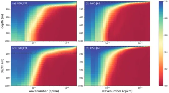
In order to characterize the depth penetration of eddy structures, we estimate for typical length scale the phase relationship between the vorticity spectral density at the surface and in the interior down to 1,000 m. This spectral correlation provides a proxy for the depth penetration of energetic surface structures (Klein et al., 2009). In Figure 9, we present the winter and summer averages of spectral correlation of vorticity in Box 1 for the two simulations. In both seasons and in the two models, we see that energetic motions with a scale larger than 100 km are strongly correlated down to a depth of about 1,000 m. On the other hand, scales smaller than 100 km penetrate less into the water column with an observed seasonality. In fact, at these scales, surface motions are correlated with the interior roughly down to 170 min winter and down to 40 min summer. Scales of motions less than 50 km tend to penetrate slightly deeper into the water column in NATL60. These summer and winter depth penetration values coincide fairly with the average mixed layer depth in the two seasons. This indicates that mixed layer instability could be a possible modulator of the vertical structure of fine-scale eddy motions. Overall, despite the differences in vertical resolution (300 vertical z levels in NATL60 and 36 hybrid isopycnal layers in HYCOM50), it is worth noting that the two simulations agree reasonably well in terms of depth penetration of eddies.
4. Spatial Variability of Eddy Scale
The spatial variability of the eddy scale is documented by computing the annual mean of the enstrophy-containing scale (L𝜁) computed from daily relative vorticity spectra for each box. The values of the mean length scale in each of the boxes for the two models are presented in Figure 10. The mean scale varies spatially with a factor of about 2 from the south to the north in the North Atlantic. This spatial vari-ability is consistent in the two models, but HYCOM50 has an annual mean scale slightly larger than NATL60 in almost all the boxes. This is consistent with what is observed in Figure 8 where typical eddy scales are larger in HYCOM50 than in NATL60.
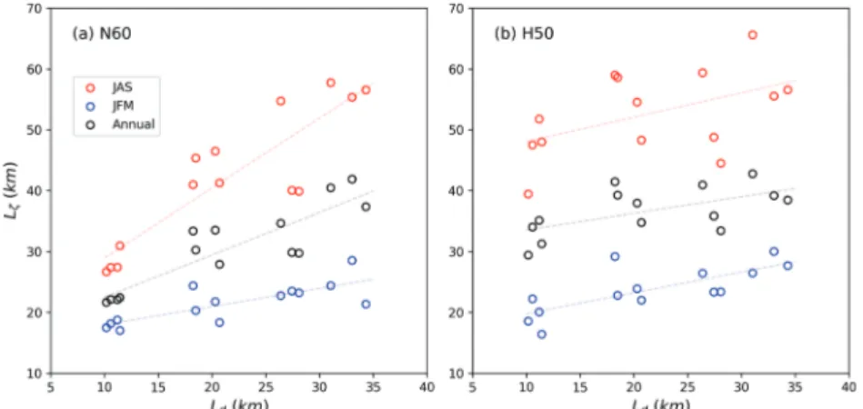
To better understand how the eddy scales compare with the Rossby radius of deformation, we present in Figure 11 a plot of the annual mean of L𝜁 versus the estimate of the first Rossby radius of deformation.
Journal of Geophysical Research: Oceans
10.1029/2019JC015827
Figure 9. (a, c) Winter and (b, d) summer averages of vorticity spectral coherence as a function of depth for NATL60 and HYCOM50 in Box 1.
The deformation radius is estimated using the GLORYS2v3 data sets following the approach highlighted in Chelton et al. (1998). The spatial variability of the annual mean scale is consistent with the estimate of the Rossby radius of deformation (Ld) with latitude (Figure 11). The length scales from HYCOM50 show less variability, and this is evident in the slope of the fitted line plot (gray dash line). The slope for the annual mean eddy scale is steeper for NATL60 (0.70) and shallower for HYCOM50 (0.27). The mean eddy scale in winter is roughly consistent in the two models, while the difference in the annual mean of the eddy scale between the two models is mainly due to the difference in the scale of eddies in summer.
Following Klocker et al. (2016), we present a regime diagram for eddies identified from the application of C11 to SSH fields. The regime diagram presents a plot of eddy scale (L𝜂) normalized by the Rossby radius of deformation against a nonlinearity parameter (r = U∕c) computed as the ratio of the root-mean-square eddy velocity (U) and the Rossby wave phase speed (c =𝛽L2
d). The eddy velocity used in this study is the
characteristic flow speed (U) within the eddy, which is defined as the average geostrophic speed within the eddy interior (Chelton et al., 2007). U = (g∕f)(A∕L), where g is the gravitational acceleration, f is the Coriolis parameter, A is the eddy amplitude, and L is the effective radius of the eddy.
Figure 11. Eddy length scale L𝜁versus first baroclinic Rossby radius Ld. (a) NATL60 and (b) HYCOM50. Dash line represents estimated regression line and each circle corresponds to a mean eddy scale in box.
The regime diagram introduces frontiers along which the dynamical behavior of eddies is expected to change significantly (Klocker et al., 2016). Two different boundaries are considered in this study: (i) rotation dom-inated (L∕Ld < 1) to stratification dominated (L∕Ld > 1) and (ii) weak to strong Rossby elasticity which is represented by the Rhines scale (Lr). Figure 12 presents a kernel density plot and describes the relative
position of eddies (as a function of eddy nonlinearity) to Ldand Lr. The first baroclinic Rossby radius of
deformation defines the length scale of variability over which the internal vortex stretching is more impor-tant than relative vorticity (Chelton et al., 1998), while the Rhines scale can be thought of as a threshold of scale at which the inverse cascade of energy is arrested. The Rhines scale can also be interpreted as the scale where the dispersion of the Rossby wave begins to dominate the ocean signal (Rhines, 1975).
Most of the detected eddies are nonlinear, and the spread of eddy nonlinearity increases with latitude. The eddy scales lie between Ldand Lr, which is consistent with the findings of Eden (2007), but the scales mostly
follow the Ldfor NATL60 (Figure 12a) while most scales in HYCOM50 are much bigger than Ld(Figure 12b). This difference follows from the argument presented in section 4 with regard to the abundance of eddies with larger scales in HYCOM50. Also, eddies in the 55◦N latitude band (gray shading) are more nonlinear in NATL60 compared to HYCOM50. One explanation could be that 55◦N latitude eddies in HYCOM50 are more elastic due to their bigger size (with respect to NATL60) and thus have smaller speed magnitude and hence smaller nonlinearity compared to NATL60. This could be interpreted as evidence of a stronger inverse cascade in HYCOM50, possibly because of the longer spin-up phase. The result from NATL60 is similar to that of Eden (2007), where the author argued that north of the 30◦N, the eddy length scale should follow the Rossby radius of deformation and not the Rhines scale.
5. Impact of Submesoscale Energy on Eddy Scale Variability
So far, we have shown that the average eddy scale varies in time across the entire North Atlantic following the seasonality of the number of SMEs. In what follows, we study the mechanism responsible for the sea-sonality of eddies from a dynamical point of view. Submesoscales are relatively more active in wintertime (Thompson et al., 2016). Their emergence is believed to be driven by mechanisms such as frontogenesis, wind-induced frontal instabilities, and mixed layer instability among other processes (McWilliams, 2016; Thomas et al., 2013). Recent studies have identified baroclinic mixed layer instability (a specific frontal instability occurring in regions with a deep mixed layer and intense horizontal buoyancy gradients) as the dominant mechanism driving the emergence of submesoscale turbulence at midlatitudes (Boccaletti et al., 2007; Capet et al., 2008; Fox-Kemper et al., 2008; Mensa et al., 2013; Sasaki et al., 2017). Also, Uchida et al. (2017), using a mesoscale-permitting ocean model on a global scale, surmised that mesoscale seasonality is a direct result of an inverse cascade of submesoscale energy generation by mixed layer instability. However, how the seasonality of submesoscales translates to the seasonality of SMEs is still unclear. This section aims to show that the increased population of SMEs in winter is directly linked to the advent of submesoscale turbulence in winter. Frontal structures that generate submesoscale eddies (Gula et al., 2016) exhibit high
Journal of Geophysical Research: Oceans
10.1029/2019JC015827
Figure 12. Kernel density plot of eddy nonlinearity (r) versus normalized eddy scale L𝜂∕Ldfor eddies identified by the
automated eddy detection algorithm. The nonlinearity parameter (r) is defined as r=U∕cfollowing Chelton et al 2007.
Colors blue, red, and gray represent eddies in the 35◦, 45◦, and 55◦latitudinal band, respectively. This regime diagram
is adapted from Klocker et al. (2016). This plot combines data corresponding to 4,680 and 3,755 detected eddy structures for (top) NATL60 and (bottom) HYCOM50 respectively.
values of relative vorticity (Held et al., 1995). We intend to show the relationship between relative vortic-ity and submesoscale eddy statistics following a correlation of the later with mixed layer depth as shown in Sasaki et al. (2017).
In order to establish the relationship between the seasonality of submesoscale energy and eddy scale season-ality, we quantify the conversion of KE through baroclinic mixed layer instability following Boccaletti et al. (2007), Fox-Kemper et al. (2008), and Capet et al. (2008). This conversion rate of available potential energy (APE) to eddy kinetic energy is defined as
PK = 1 h∫ −h 0 ⟨w ′b′⟩ x𝑦dz. (2)
Figure 13. Time series of available potential energy, PK (blue line) and mixed layer depth, MLD (black line) for NATL60. The two dashed vertical lines represent the beginning and the end of winter: JFM.—These results are based on the year 2012/2013 of NATL60 simulation and are therefore not representative of a climatology state.
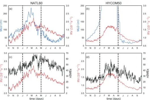
Figure 14. Time series of mixed layer depth, MLD (thin black line), root-mean-square of the surface relative vorticity RV (red line) and the number of submesoscale eddies (thick black line) in Box 1 for (a, c) NATL60 and (b, d)
HYCOM50 data sets. nSMEs (daily number of L𝜂with a scale between 10 and 50 km). The two dashed vertical lines
represent the beginning and the end of winter: JFM.
The parameters h, w, and b represent the mixed layer depth, vertical velocity, and buoyancy gradient, respectively. The prime sign[′]
indicates the small-scale component of the flow obtained by applying Lanc-zos windowing (with a cutoff frequency of 0.0125 and window size of 80 grid points) method to the two-dimensional fields of vertical velocity (w) and buoyancy (b).
Figure 15. Time series of mixed layer depth, MLD (thin black line), root-mean-square of the surface relative vorticity RV (red line) and the number of submesoscale eddies (thick black line) in Box 11 for (a, c) NATL60 and (b, d)
HYCOM50 data sets. nSMEs (daily number of L𝜂with a scale between 10 and 50 km). The two dashed vertical lines
Journal of Geophysical Research: Oceans
10.1029/2019JC015827
Figure 16. March (blue line) and September (red line) profile of w′b′in (left) Box 1 and (right) Box 11 for NATL60 (thick line) and HYCOM50 (dashed line). Thick dots represent mixed layer depth.
Figure 13 presents the time series of mixed layer depth (MLD) (blue line) and PK (black line) in Box 1 and Box 11 for NATL60. These two quantities are correlated with similar peaks in wintertime. This is consistent with previously published results of Boccaletti et al. (2007) and Sasaki et al. (2014), and this underscores mixed layer instability as the major driver for the emergence of submesoscale in winter.
We show similar time series for MLD (blue line), RV (red line) and daily counts of SMEs (thick black line) in Figures 14 and 15 for Box 1 and Box 11, respectively. Indeed, Figures 14a, 14b and 15a, 15b highlight how mixed layer instability drives the evolution of relative vorticity with a peak value in winter. An abrupt decay of MLD is observed in late winter that is not observed for RV. A similar result was recorded by Sasaki et al. (2017), and the authors attributed this difference in MLD and RV (starting in late winter) to the evolution of RV in two-dimensional turbulent flow in free decay after an abrupt decay of MLD. This implies that the dynamics immediately after wintertime is characterized by an inverse cascade of energy. This inverse cas-cade is evident in the subsequent decline in the number of submesoscale eddies in late winter (Figures 14c, 14d and 15c, 15d). It is, however, worth mentioning that SMEs and RV show a strong correlation with a similar peak in winter.
Figure 16 presents the vertical profile of eddy buoyancy fluxes⟨w′b′⟩ in March and September for Box 1 and Box 11. We see seasonality in the profiles, and this is associated with changes in mixed layer depth. The magnitude of⟨w′b′⟩ in March is higher compared to September for the two simulations. A higher ⟨w′b′⟩ is responsible for feeding the growth and emergence of submesoscales eddies in winter. This growth is, however, region dependent. The winter-summer change in APE in Box 1 is about a factor of 3 higher than Box 11 for both NATL60 and HYCOM50.
6. Conclusion
The spatial and temporal variability of the typical size of oceanic eddies smaller than 100 km is investigated in this study using two submesoscale-permitting ocean model simulations of the North Atlantic; NATL60 and HYCOM50. The scale of oceanic eddies shows a substantial temporal and spatial variability, as reflected in the enstrophy-containing scale estimated from the vorticity wave number spectra. Our analysis reveals that the increased population of submesoscale eddies (10–50 km), driven by mixed layer instability in win-tertime, is responsible for the seasonality of the scales of eddies in the North Atlantic. The winter/summer difference in the mean eddy scale is about a factor of 2 in favor of summer. The map of mean eddy scale reveals that the spatial variability of eddy length scale is consistent with the latitudinal dependence of the first Rossby radius of deformation and that most of the eddies 30◦N of the North Atlantic are nonlinear in nature with a wider nonlinearity spread in the 55◦N latitudinal bands. There are concerns as to the size of the eddies identified in the models. We nonetheless stress that the eddies are relatively smaller in NATL60 than in HYCOM50, and this is possibly a consequence of NATL60 short spin-up phase (6 months) and smaller
inverse energy cascade. In light of that, a longer run of NATL60 is recommended for future study to allow enough time for the simulated eddies to equilibrate. In terms of eddy penetration, we found that at scales less than 100 km, the vertical structures of energetic eddy motion (diagnosed from the spectral coherence of vorticity) vary seasonally as a function of the mixed layer depth. In fact, the depth penetration of eddies with scales<50 km is confined to the mixed layer. This further highlights how mixed layer instability modulates fine-scale dynamics.
While the focus of this study is to investigate eddy scale variability, we also examined the ability of NATL60 and HYCOM50 as a virtual observation scene for the SWOT mission. Following the analysis presented in this study and despite the model differences in terms of numerics, parameterization scheme, and verti-cal resolution, the statistics of eddy sverti-cale and the vertiverti-cal structure of eddy motions captured by the two models are comparable. We can reasonably conclude that both NATL60 and HYCOM50 have the capabil-ity to resolve and characterize fine-scale dynamics down to 15-km scales in the North Atlantic and that the fine-scale dynamics predicted by the models are a robust feature of this class of kilometric ocean models. This is key for the SWOT mission because information about eddy scale variability from these simulations (with respect to their horizontal resolution) is useful for the calibration of inversion techniques for esti-mating two-dimensional maps of SSH from SWOT data. This knowledge of eddy scale variability will also be useful for improving the eddy parameterization schemes of ocean models. Also, submesoscale eddies are visible in surface chlorophyll observations from high-resolution remote sensing data (Choi et al., 2019; McWilliams, 2016), and recent studies have argued that vertical transport due to submesoscales plays an important pathway in supplying nutrients to the euphotic layer (Levy et al., 2018; Zhang et al., 2019). Given that these oceanic motions and their scales undergo strong seasonality as clearly shown in this study, their contribution to vertical transport of nutrients might suffer the same seasonality, and this has implications for climates models that parameterize this process of upwelling by submesoscale motions.
References
Amores, A., Jorda, G., Arsouze, T., & Le Sommer, J. (2018). Up to what extent can we characterize ocean eddies using present-day gridded altimetric products? Journal of Geophysical Research: Oceans, 123, 7220–7236. https://doi.org/10.1029/2018JC014140
Amores, A., Jorda, G., & Monserrat, S. (2019). Ocean eddies in the Mediterranean Sea from satellite altimetry: Sensitivity to satellite track location. Frontiers Marine Science, 10, 68. https://doi.org/10.3389/fmars.2019.00703
Bates, M., Tulloch, R., Marshall, J., & Ferrari, R. (2014). Rationalizing the spatial distribution of mesoscale eddy diffusivity in terms of mixing length theory. Journal of Physical Oceanography, 44(6), 1523–1540. https://doi.org/10.1175/JPO-D-13-0130.1
Boccaletti, G., Ferrari, R., & Fox-Kemper, B. (2007). Mixed layer instabilities and restratification. Journal of Physical Oceanography, 37(9), 2228–2250. https://doi.org/10.1175/JPO3101.1
Brannigan, L., Marshall, D. P., Naveira-Garabato, A., & George Nurser, A. J. (2015). The seasonal cycle of submesoscale flows. Ocean
Modelling, 92, 69–84. https://doi.org/10.1016/j.ocemod.2015.05.002
Bryan, F. O. (2008). Introduction: Ocean modeling-eddy or not. Gophysical Monthly Series, 177, 1–4. https://doi.org/10.1029/177GM02 Buckingham, C. E., Natasha, L., Stephen, B., Tom, R., Alan, G., Julien, L. S., et al. (2019). The contribution of surface and submesoscale
processes to turbulence in the open ocean surface boundary layer. Journal of Advances in Modeling Earth Systems, 11, , 4066–4094. https://doi.org/10.1029/2019MS001801
Callies, J., Ferrari, R., Klymak, J. M., & Gula, J. (2015). Seasonality in submesoscale turbulence. Nature Communication, 6, 6862. https:// doi.org/10.1038/ncomms7862
Callies, J., Flierl, G., Ferrari, Ra., & Fox-Kemper, B. (2015). The role of mixed-layer instabilities in submesoscale turbulence. Journal of
Fluid Mechanics, 788, 5–41. https://doi.org/10.1017/jfm.2015.700
Capet, X., Campos, E. J., & Paiva, A. M. (2008). Submesoscale activity over the Argentinian shelf. Geophysical Research Letters, 35, L15605. https://doi.org/10.1029/2008GL034736
Chassignet, E. P., & Xu, X. (2017). Impact of horizontal resolution (1/12◦to 1/50◦) on Gulf Stream separation, penetration, and variability.
Journal of Physical Oceanography, 47(8), 1999–2021. https://doi.org/10.1175/JPO-D-17-0031.1
Chelton, D. B., DeSzoeke, R., Schlax, M., El Naggar, K., & Siwertz, N. (1998). Geographical variability of the first baroclinic Rossby radius of deformation. Journal of Physical Oceanography, 28(3), 433–460. https://doi.org/10.1175/1520-0485(1998)028h0433:GVOTFBi2.0.CO;2 Chelton, D. B., Schlax, M. G., & Samelson, R. M. (2011). Global observations of nonlinear mesoscale eddies. Progress in Oceanography,
91(2), 167–216. https://doi.org/10.1016/j.pocean10.1016/j.pocean
Chelton, D. B., Schlax, M. G., Samelson, R. M., & DeSzoeke, R. (2007). Global observations of large oceanic eddies. Geophysical Research
Letters, 34, L15606. https://doi.org/10.1029/2007GL030812
Choi, J., Park, Y. G., Kim, W., & Kim, Y. H. (2019). Characterization of submesoscale turbulence in the East/Japan Sea using geostationary ocean color satellite images. Geophysical Research Letters, 46, 8214–8223. https://doi.org/10.1029/2019GL083892
Ducet, N., & Traon, P. L. (2001). A comparison of surface eddy kinetic energy and Reynolds stresses in the Gulf Stream and the Kuroshio Current systems from merged TOPEX/Poseidon and ERS-1/2 altimetric data. Journal of Geophysical Research, 106, 16,603–16,622. https://doi.org/10.1029/2000JC000205
Ducousso, N., Le Sommer, J., Molines, J. M., & Bell, M. (2017). Impact of the symmetric instability of the computational kind at mesoscale-and submesoscale-permitting resolutions. Ocean Modelling, 120, 18–26. https://doi.org/10.1016/j.ocemod.2017.10.006
Dufau, C., Orsztynowicz, M., G., D., R., M., & P.Y., L. T. (2016). Mesoscale resolution capability of altimetry: Present and future. Journal of
Geophysical Research: Oceans, 121, 4910–4927. https://doi.org/10.1175/JPO-D-11-0240.1
Dussin, R., Barnier, B., Brodeau, L., & Molines, J. M. (2018). The making of the DRAKKAR forcing set DFS5. https://doi.org/10.5281/ zenodo.1209243
Acknowledgments
Adekunle Ajayi was supported by the Universite Grenoble Alpes (AGIR research grant). Aurélie Albert was supported by the CMEMS (Global High-Resolution MFC 22-GLO-HR). Julien Le Sommer and Emmanuel Cosme would like to acknowledge the support from CNES and ANR (ANR-17-CE01-0009-01). This work is a contribution to the SWOT mission Science Team. Eric Chassignet and Xiaobiao Xu are supported by the Office of Naval Research (Grant N00014-15-1-2594) and the NSF Physical Oceanography Program (Award 1537136). HYCOM50 and NEMO-NATL60 data can be accessed at ftp://ftp.hycom.org/pub/xbxu/ ATLb0.02/ and http://meom-group. github.io/swot-natl60/access-data. html, respectively.
Journal of Geophysical Research: Oceans
10.1029/2019JC015827
Eden, C. (2007). Eddy length scales in the North Atlantic Ocean. Journal of Geophysical Research, 112, C06004. https://doi.org/10.1029/ 2006JC003901
Fox-Kemper, B., Ferrari, R., & Hallberg, R. (2008). Parameterization of mixed layer eddies. Part I: Theory and diagnosis. Journal of Physical
Oceanography, 6(38), 1145–1165.
Fu, L. L., Chelton, D. B., Le Traon, P. Y., & Morrow, R. (2010). Eddy dynamics from satellite altimetry. Oceanography, 23(4), 14–25. https:// doi.org/10.5670/oceanog.2010.02
Fu, L. L., & Ubelmann, C. (2014). On the transition from profile altimeter to swath altimeter for observing global ocean surface topography.
Journal Atmosphere Oceanic Technolology, 31, 560–568. https://doi.org/10.1175/JTECH-D-13-00109.1
Gula, J., Molemaker, J., & McWilliams, J. C. (2016). Submesoscale dynamics of a Gulf Stream frontal eddy in the South Atlantic Bight.
Journal of Physical Oceanography, 46(1), 305–325. https://doi.org/10.1175/JPO-D-14-0258.1
Held, I. M., Pierrehumbert, R. T., Garner, S. T., & Swanson, K. L. (1995). Surface quasigeostrophic dynamics. Journal of Fluid Mechanics,
282, 1–20.
Klein, P., Isem-Fontanet, J., Lapeyre, G., Roullet, G., Danioux, E., Chapron, B., et al. (2009). Diagnosis of vertical velocities in the upper ocean from high resolution sea surface height. Geophysical Research Letters, 36, L12603. https://doi.org/10.1029/2009GL038359 Klocker, A., & Abernathey, R. (2014). Global patterns of mesoscale eddy properties and diffusivities. Journal of Physical Oceanography,
44(3), 1030–1046. https://doi.org/10.1175/JPO-D-13-0159.1
Klocker, A., Marshall, D. P., Keating, S. R., & Read, P. L. (2016). A regime diagram for ocean geostrophic turbulence. Journal of the Royal
Meteorological Society. https://doi.org/10.1002/qj.2833
Le Traon, P. Y., Rouquet, M. C., & Boissier, C. (1990). Spatial scales of mesoscale variability in the North Atlantic as deduced from Geosat data. Journal of Geophysical Research, 95, 20,267. https://doi.org/10.1029/JC095iC11p20267
Levy, M., Franks, P. J. S., & Smith, K. S. (2018). The role of submesoscale currents in structuring marine ecosystems. Geophysical Research
Letters, 9, 4758. https://doi.org/10.1038/s41467-018-07059-3
McWilliams, J. C. (2016). Submesoscale currents in the ocean. Proceedings of the Royal Society, A 472, 20160117. https://doi.org/10.1098/ rspa.2016.0117
Mensa, J. A., Garraffo, Z., Griffa, A., Ozgokmen, T. M., Haza, A., & Veneziani, M. (2013). Seasonality of the submesoscale dynamics in the Gulf Stream region. Ocean Dynamics, 63, 923–941.
Morris, S. C., & Foss, J. F. (2005). Vorticity spectra in high Reynolds number anisotropic turbulence. Physics of Fluids, 17(8), 1–4. https:// doi.org/10.1063/1.1989387
Moum, J. N. (1996). Energy-containing scales of turbulence in the ocean thermocline. Journal of Geophysical Research, 101(C6), 14,095–14,109. https://doi.org/10.1029/96JC00507
Qiu, B., Chen, S., Klein, P., Sasaki, H., & Sasai, Y. (2014). Seasonal mesoscale and submesoscale eddy variability along the North Pacific subtropical countercurrent. Journal of Physical Oceanography, 44(12), 3079–3098. https://doi.org/10.1175/JPO-D-14-0071/.1 Rhines, P. B. (1975). Waves and turbulence on a beta-plane. Journal of Fluid Mechanic, 69, 417–443. https://doi.org/10.1017/
S0022112075001504
Rocha, C. B., Gille, S. T., Chereskin, T. K., & M., D. (2016). Seasonality of submesoscale dynamics in the Kuroshio Extension. Geophysical
Research Letters, 43, 11,304–11,311. https://doi.org/10.1002/2016GL071349
Sasaki, H., Klein, P., Qiu, B., & Sasai, Y. (2014). Impact of oceanic scale- interactions on the seasonal modulation of ocean dynamics by the atmosphere. Nature Communication, 5, 5636. https://doi.org/10.1038/ncomms6636
Sasaki, H., Klein, P., Sasai, Y., & Qiu, B. (2017). Regionality and seasonality of submesoscale and mesoscale turbulence in the North Pacific Ocean. Ocean Dynamics, 67, 1195–1216. https://doi.org/10.1007/s10236-017-1083-y
Scott, R. B. (2001). Evolution of energy and enstrophy containing scales in decaying, two-dimensional turbulence with friction. Physics of
Fluids, 13(9), 2739–2742.
Stammer, D. (1997). Global characteristics of ocean variability estimated from regional TOPEX/ POSEIDON altimeter measurements.
Journal of Physical Oceanography, 27, 1743–1769. https://doi.org/10.1175/1520-0485(1997)027h1743:GCOOVEi2.0.CO;2
Stammer, D., & Böning, C. W. (1992). Mesoscale variability in the Atlantic Ocean from Geosat Altimetry and WOCE high-resolution numerical modeling. (Vol. 22) (No. 7).
Thomas, L. N., Tandon, A., & Mahadevan, A. (2013). Submesoscale Processes and Dynamics. In M. W. Hecht & H. Hasumi (Eds.), Ocean
Modeling in an Eddying Regime. https://doi.org/10.1029/177GM04
Thompson, A., Lazar, A., Buckingham, C., Naveira Garabato, A., Damerell, G. M., & Heywood, K. J. (2016). Open-ocean submesoscale motions: A full seasonal cycle of mixed layer instabilities from Gliders. Journal of Physical Oceanography, 46, 1285–1307. https://doi. org/10.1175/JPO-D-15-0170.1
Uchida, T., Abernathey, R., & Smith, S. (2017). Seasonality of eddy kinetic energy in an eddy permitting global climate model. Ocean
Modelling, 118, 41–58. https://doi.org/10.1016/j.ocemod.2017.08.006
Uppala, S. M., Kållberg, P. W., Simmons, A. J., Andrae, U., da Costa Bechtold, V., Fiorino, M., et al. (2005). The ERA-40 re-analysis. Quarterly
Journal of the Royal Meteorological Society, 131(612), 2961–3012. https://doi.org/10.1256/qj.04.176
Zhang, Z., Qiu, B., Klein, P., & Travis, S. (2019). The influence of geostrophic strain on oceanic ageostrophic motion and surface chlorophyll.