HAL Id: hal-03106874
https://hal.archives-ouvertes.fr/hal-03106874
Submitted on 12 Jan 2021
HAL is a multi-disciplinary open access
archive for the deposit and dissemination of
sci-entific research documents, whether they are
pub-lished or not. The documents may come from
teaching and research institutions in France or
abroad, or from public or private research centers.
L’archive ouverte pluridisciplinaire HAL, est
destinée au dépôt et à la diffusion de documents
scientifiques de niveau recherche, publiés ou non,
émanant des établissements d’enseignement et de
recherche français ou étrangers, des laboratoires
publics ou privés.
multispectral image fusion with inter-image variability
Ricardo Borsoi, Clémence Prévost, Konstantin Usevich, David Brie, José
Bermudez, Cédric Richard
To cite this version:
Ricardo Borsoi, Clémence Prévost, Konstantin Usevich, David Brie, José Bermudez, et al..
Cou-pled tensor decomposition for hyper spectral and multispectral image fusion with inter-image
vari-ability.
IEEE Journal of Selected Topics in Signal Processing, IEEE, 2021, 15 (3), pp.702-717.
�10.1109/JSTSP.2021.3054338�. �hal-03106874�
Coupled Tensor Decomposition for
Hyperspectral and Multispectral Image
Fusion with
Inter-image
Variability
Ricardo A. Borsoi, Clémence Prévost, Konstantin Usevich, David Brie, José C. M. Bermudez, Cédric Richard
Abstract—Coupled tensor approximation has recently emerged as a promising approach for the fusion of hyperspectral and multispectral images, reconciling state of the art performance with strong theoretical guarantees. However, tensor-based approaches previously proposed assume that the different observed images are acquired under exactly the same conditions. A recent work proposed to accommodate inter-image spectral variability in the image fusion problem using a matrix factorization-based formulation, but did not account for spatially-localized variations. Moreover, it lacks theoretical guarantees and has a high associated computational complexity. In this paper, we consider the image fusion problem while accounting for both spatially and spectrally localized changes in an additive model. We first study how the general identifiability of the model is impacted by the presence of such changes. Then, assuming that the high-resolution image and the variation factors admit a Tucker decomposition, two new algorithms are proposed – one purely algebraic, and another based on an optimization procedure. Theoretical guarantees for the exact recovery of the high-resolution image are provided for both algorithms. Experimental results show that the proposed method outperforms state-of-the-art methods in the presence of spectral and spatial variations between the images, at a smaller computational cost.
Index Terms—Hyperspectral data, multispectral data, inter-image variability, super-resolution, image fusion, tensor decomposition.
I. INTRODUCTION
Hyperspectral (HS) cameras are able to acquire images with very high spectral resolution. However, the fundamental compromise between signal-to-noise ratio, spatial resolution, and spectral resolution means that their spatial resolution is usually low [1]. Multispectral (MS) devices, on the other hand, are able to achieve a much higher spatial resolution
This work was partly supported by the ANR (Agence Nationale de Recherche) under grant LeaFleT (ANR-19-CE23-0021), by the National Council for Scientific and Technological Development (CNPq) under grants 304250/2017-1, 409044/2018-0, 141271/2017-5 and 204991/2018-8, by the Foundation for Research Support of the State of Rio Grande do Sul (FAPERGS) under grant 19/2551-0001844-4.
We also thank the GdR CNRS ISIS for supporting the collaboration between R.A. Borsoi and C. Prévost, K. Usevich and D. Brie through a bourse de mobilité.
R.A. Borsoi is with the Department of Electrical Engineering, Federal University of Santa Catarina (DEE–UFSC), Florianópolis, SC, Brazil, and with the Lagrange Laboratory, Université Côte d’Azur, Nice, France. e-mail: [email protected].
C. Prévost, K. Usevich and D. Brie are with Centre de Recherche en Automatique de Nancy (CRAN), Université de Lorraine, CNRS, Vandoeuvre-lès-Nancy, France. e-mail: [email protected].
J.C.M. Bermudez is with the DEE–UFSC, Florianópolis, SC, Brazil. e-mail: [email protected].
C. Richard is with the Université Côte d’Azur, Nice, France (e-mail: [email protected]), Lagrange Laboratory (CNRS, OCA).
since they contain only a small number of spectral bands. An approach that attempts to circumvent the physical limitations of imaging sensors consists in combining HS and MS images (MSI) of the same scene to obtain images with high spatial and spectral resolution, in a multimodal image fusion problem [2], commonly referred to as hyperspectral super resolution.
Different algorithms have been proposed to solve this problem. Early approaches were based on component substitution or on multiresolution analysis, which attempt to extract high-frequency spatial details from the MSI and combine them with the HS image (HSI) [3], [4]. Subspace-based formulations have later received a significant amount of interest as they explore the natural representation of the pixels in an HSI as the linear combination of a small number of spectral signatures [2], [5], [6]. Different algorithms have been proposed following this approach using, e.g., Bayesian formulations [7] or sparse representations on learned dictionaries [8], and different kinds of matrix factorization formulations employing sparse and spatial regularizations [9], [10], or estimating both the basis vectors and their coefficients blindly/unsupervisedly from the images [11].
The natural representation of HSIs and MSIs as 3-dimensional tensors has been successfully exploited for hyperspectral unmixing, denoising [12]–[15] and super-resolution. Superior super-resolution performance and exact recovery guarantees have been obtained using this formulation [16], [17].
The image fusion problem was formulated in [16] as a coupled tensor approximation problem. Assuming that the high resolution (HR) image admits a low-rank canonical polyadic decomposition (CPD), the problem was solved using an alternating optimization strategy. The recovery of the correct HR image (HRI) was shown to be guaranteed provided that the CPD of the MSI is identifiable, and state of the art performance was achieved. A recent work extended this approach by assuming the high resolution images to follow a block term decomposition (BTD), which shows a closer connection to the physical mixing model when compared to the CPD [18]. A simpler approach was later proposed in [19] by requiring only the computation of one CPD of the MSI and a singular value decomposition (SVD) of the HSI.
A Tucker decomposition-based approach was later considered in [17], [20]. Closed form SVD-based algorithms were proposed for the image fusion problem, achieving results comparable to [16] at a very small computational complexity; exact recovery guarantees were also provided. A coupled
Tucker approximation was also considered in [21] using an alternating optimization approach and employing a sparsity regularization on the elements of the core tensor. This work was later extended by incorporating the piecewise smoothness of the reconstructed image tensor by using a Total Variation regularization along each of its modes [22].Another approach considered the CPD of non-local similar patch tensors to explore the non-local redundancy of the image [23]. A different non-local approach was also proposed in [24] by using a recent definition of the nuclear norm of order-3 tensors.
Most existing algorithms, however, share a common limita-tion: they assume that the HSI and the MSI are acquired under the same conditions. However, despite the short revisit cycles provided by the increasing number of optical satellites orbiting the Earth (e.g. Sentinel, Orbview, Landsat and Quickbird mis-sions), the number of platforms carrying both HS and MS sen-sors is still considerably limited [25], [26]. This makes com-bining HS and MS observations acquired on board of different satellites of great interest to obtain HRIs [27], [28]. Images acquired at different time instants can be impacted by, e.g., illumination, atmospheric or seasonal changes. This may result in significant variations between the HSI and the MSI [29], negatively impacting traditional image fusion algorithms.
Recently, a method was proposed to combine HSIs and MSIs accounting for seasonal (inter-image) spectral variability [30]. Using a low-rank matrix formulation, the set of spectral basis vectors of the HRIs underlying the HS and the MS observations are allowed to be different from each other, with variations introduced by a set of multiplicative scaling factors [31]. This algorithm led to significant performance improvements when the HSI and MSI are subject to spatially uniform seasonal or acquisition variations. However, it does not account for spatially localized changes commonly seen in practical scenes [29]. Moreover, the algorithm in [30] presented high computation times and does not offer any theoretical guarantees.
In this paper, we propose a tensor-based image fusion formulation that accounts for localized spatial and spectral changes between the HSI and MSI. A general observation model is considered, in which the HRI underlying the MSI admits an additive variability term to account for changes between the scenes. Studying the general identifiability of this model, we show that this variability term can only be identified in general up to its smooth structure (which is defined according to the degradation operators). To introduce additional a priori information and mitigate the ambiguity associated with the proposed model, both the HRI and the additive perturbations are assumed to have low multilinear rank (i.e., to admit a Tucker decomposition). Two algorithms are then proposed, one totally algebraic and another based on an optimization procedure. Theoretical guarantees for the exact recovery of the HRI are provided for both. Simulation results show that the proposed optimization-based algorithm yields superior performance at a considerably lower computational cost when compared to [30], especially when spatially localized variability is considered.
II. TENSORS–BACKGROUND
A. Notation and definitions
An order-3 tensor T P RN1ˆN2ˆN3is an N
1ˆN2ˆN3array
whose elements are indexed by rT sn1,n2,n3. Each dimension
ofan order-3 tensoris called a mode. A mode-k fiber of tensor T is the one-dimensional subset of T which is obtained by fixing all but one of the three modes – the k-th dimension. Similarly, a slab or slice of a tensor T is a matrix whose elements are the two-dimensional subset of T obtained by fixing all but two of its modes. Operator vecp¨q represents the standard matrix column-major vectorization, or tensor vectorization. The (left) pseudo-inverse of matrix X is denoted by X:. We denote scalars by lowercase (x) or uppercase (X) plain font, vectors and matrices by lowercase (x) and uppercase (X) bold font, respectively, and order-3 tensors by calligraphic plain font (T ) or using the blackboard Greek al-phabet (Θ). In the following, we review some useful operations of multilinear (tensor) algebra that will be used in the rest of the manuscript (see, e.g., [32], [33] for more details). Definition 1. The mode-k product between a tensor T and a matrix B produces a tensor U that is evaluated such that each mode-k fiber of T is multiplied by B. For instance, the mode-2 product between T P RN1ˆN2ˆN3
and B P RM2ˆN2 produces a tensor U P RN1ˆM2ˆN3,
denoted by U “ T ˆ2 B. Its elements are accessed as
rU sn1,m2,n3 “
řN2
i“1rT sn1,i,n3rBsm2,i , m2“ 1, . . . , M2.
Note that the mode-k product has the following properties: T ˆiA ˆjB “ T ˆjB ˆiA , i ‰ j , (1)
T ˆkA ˆkB “ T ˆk`AB˘ . (2)
Definition 2. The full multilinear product is denoted by 0T ; B1, B2, B3
8
, and consists of a series of successive mode-k products, for k P t1, 2, 3u, between a tensor T and matrices B1, B2 and B3, respectively, and is expressed as
T ˆ1B1ˆ2B2ˆ3B3.
Definition 3. The mode-k matricization of an order-3 tensor T P RN1ˆN2ˆN3, denoted byT
pkq, arranges its mode-k fibers
to be the columns of the resulting matrixTpkqP RNkˆN`Nm,
k, `, m P t1, 2, 3u, k ‰ ` ‰ m, where the nk-th row of Tpkq
consists of the vectorization of the slice of T obtained by fixing the index of the k-th mode of T as nk.
Definition 4. We define by tSVDRpXq the operator which
returns a matrix containing the R left singular vectors associated with the largest singular values of the matrixX. B. Tensor decompositions
The Tucker decomposition is able to represent an order-3 tensor T P RN1ˆN2ˆN3 compactly, using a set of factor
matrices given by Bi P RNiˆKi, i P t1, 2, 3u and a small
core tensor G P RK1ˆK2ˆK3, as [33]
T “0G; B1, B2, B38 . (3)
The tuple pK1, K2, K3q is called the multilinear rank of
T . Each value Ki is also equal to the rank of the mode-i
The Tucker decomposition allows the rank along each mode of the tensor to be different (i.e., Ki ‰ Kj) [34]. This
property can be very useful since it allows one to set a higher rank to specific modes of the decomposition in order to adequately represent the data diversity while still keeping the model low rank.
The matricizations and vectorization of a tensor T following the Tucker decomposition (3) are given by [33]:
vecpT q “ pB3b B2b B1q vecpGq , (4)
Tp1q“ B1Gp1qpB3b B2qJ, (5)
Tp2q“ B2Gp2qpB3b B1qJ, (6)
Tp3q“ B3Gp3qpB2b B1qJ. (7) The Tucker decomposition can be computed using fast algorithms such as the high-order SVD [35].
Another classic tensor decomposition is the Canonical Polyadic Decomposition (CPD) [33]. The CPD enjoys uniqueness properties under very mild conditions, and its rank can exceed the dimensions of the tensor. However, it is also more difficult to compute, and the same rank value is used to represent all modes of the tensor.
The Block Term Decomposition (BTD) generalizes CPD and Tucker, and allows us to combine benefits from both approaches [36].Specifically, the BTD of an order-3 tensor T is defined as a sum of rank-pK1,r, K2,r, K3,rq terms as [36]:
T “
R
ÿ
r“1
0Gr; Br,1, Br,2, Br,38 , (8)
where Gr, Br,1, Br,2, and Br,3, for r “ 1, . . . , R, are
the core tensors and the factors corresponding to each mode of T . Differently from the Tucker decomposition, the BTD additionally requires the selection of parameter R (number of blocks), and can be more costly to compute. However, the BTD benefits from uniqueness results which, although not as strong than those of the CPD, are still interesting for many applications [36, Section 5]. These results will prove very important to derive the recoverability guarantees for the algorithm in Section V. Note that in the CPD can be viewed as a special case of the BTD with R “ 1.
III. PROPOSED MODEL AND ITS UNDETERMINACIES
A. The imaging model
Let an HSI with high spectral resolution and low spatial res-olution be represented as an order-3 tensor YhP RN1ˆN2ˆLh,
where N1 and N2 are the spatial and Lh the spectral
dimen-sions. Similarly, an MSI with high spatial and low spectral resolution is denoted by an order-3 tensor YmP RM1ˆM2ˆLm,
where M1ą N1 and M2ą N2 are the spatial and Lmă Lh
the spectral dimensions. Both the HSI and the MSI are assumed to be degraded versions of a tensor Z P RM1ˆM2ˆLh
` ,
with high spectral and spatial resolutions. This degradation process is commonly described as [16], [17], [20], [21]:
Yh“ Z ˆ1P1ˆ2P2` Eh, (9)
Ym“ Z ˆ3P3` Em, (10)
where tensors Em P RM1ˆM2ˆLm and Eh P RN1ˆN2ˆLh
represent additive noise. The matrix P3 P RLmˆLh contains
Figure 1. Proposed imaging model. The observed HSI and MSI are acquired under different conditions or at different time instants. Their underlying HRIs, represented by tensors Zhand Zm, respectively, can be different from each
other due to the effect of spectral and acquisition variations, as well as scenery
changes. The changes occurring between the HRIs Zhand Zmare
repre-sented using an additive tensor Ψ which captures variability and changes, and both the HRI and the variability tensors are assumed to have low Tucker rank.
the spectral response functions (SRF) of each band of the multispectral sensor, and matrices P1 P RN1ˆM1
and P2 P RN2ˆM2 represent the spatial blurring and downsampling in the hyperspectral sensor, which we assume to be separable for each spatial dimension as previously done in, e.g., [16], [17], [20], [21]. Note that since the mode-k product obeys (1), the choice of the ordering of P1 and
P2 in (9) does not affect the result. To make notation more
convenient, we also denote the (linear) spatial and spectral degradation operators more compactly as
P1,2pT q “ T ˆ1P1ˆ2P2, (11)
P3pT q “ T ˆ3P3. (12)
Most previous works consider that Yh and Ym are
ac-quired under the same conditions, implicitly assuming that no variability or changes occur between the images. However, when the HSI and MSI are not acquired from the same mission/instrument and at the same time, the scene which un-derlies the (degraded) observations Yhand Ymcan be subject
to significant changes, referred to as inter-image variability1, which include spatial and spectral variations as illustrated in Fig. 1. Spectral variations originate from different chemical, atmospheric, illumination or seasonal conditions between the scenes [29], [37], [38], and are typical even under short acqui-sition time differences. Spatial variations, on the other hand, occur due to, e.g., some regions of the scene being affected unequally by seasonal effects (which are strongly material-dependent [29]) or due to the sudden insertion/removal of an object [39]. Spatial variations can be very prominent when large acquisition time differences are considered. These effects are not accounted for in the majority of the existing algorithms, what motivates the development of more flexible models.
Recently, spatially uniform spectral variability has been considered in [30]. The image fusion problem was formulated as a matrix factorization problem, and the (multiplicative) spectral variability as well as the spatial coefficients were
1Here, variability should not be confused with the spectral variability
estimated from the observed images. However, this work still did not address two fundamental problems: 1) How to account for both spatial and spectral variability and 2) what theoretical guarantees can be offered for the recovery of the HRI and (possibly) of the variability factors under these more challenging conditions.
To address these issues, we adopt a more general approach by considering two different HRIs Zh P RM`1ˆM2ˆLh and
ZmP RM`1ˆM2ˆLh, both with high spectral and spatial
resolu-tions, underlying the observed HSI and the MSI, respectively. This leads to the following extension of model (9)–(10):
Yh“P1,2pZhq ` Eh, (13)
Ym“P3pZmq ` Em. (14) The tensors Zh and Zm represent the underlying HRIs
of the observed scene under different acquisition conditions and at possibly different times. To account for inter-image variability, the HRIs are related to each other as follows:
Zm“Zh` Ψ, (15)
where Ψ P RM1ˆM2ˆLh is an additive variability tensor
representing changes between the scenes. By introducing Ψ, model (15) makes the inter-image variability between the HSI and the MSI explicit.
Considering the variability model (15) along with (13)– (14), we obtain the following observation model for the acquired HSI and MSI:
Yh“P1,2pZhq ` Eh, (16)
Ym“P3pZh` Ψq ` Em. (17) In the following, Zh and Ψ will be referred to as the HRI
and the variability tensor, respectively.
B. The image fusion problem and its undeterminacies The image fusion problem in this case consists in recovering Ψ and Zh from the observed images Yh and Ym.
More precisely, #
findZhP ΩZ and Ψ P ΩΨ,
such that equations (16)–(17) are satisfied. (18) The sets ΩZ Ď RM1ˆM2ˆLh and ΩΨ Ď RM1ˆM2ˆLh denote
prior information about the HRI and the variability factor, respectively.
Since the number of unknowns is significantly greater than the number of observations, problem (18) is severely ill-posed and additional a priori information about the structure ofZh
and Ψ must be introduced through the sets ΩZand ΩΨin order
to obtain a stable recovery. Common information that has been used to construct ΩZ includes spatial (piecewise-)
smooth-ness [10], low matrix (spectral) rank [11], [30], low tensor rank [16], [17], [23], and non-local spatial information [21].
The choice of prior information in ΩZ and ΩΨ turns to the
question of whether assuming additional structure over the pair pZh, Ψq makes these variables identifiable from the
observa-tions pYh, Ymq. Recent works in HS-MS image fusion
advo-cates for a low-rank tensor model [16], [17], [20]. However, the case at hand is more challenging because of the additional variability Ψ, which makes the model more ambiguous.
In many inverse problems such as matrix or tensor factor-ization, dictionary learning and blind deconvolution, identifia-bility of the underlying variables often can only be defined up to some fundamental ambiguities. Transformation groups and equivalence classes [40] can be used to precisely define which sets of solutions can generate each possible observations. These ideas can be leveraged to characterize some of the fundamental ambiguities associated with the model (16)–(17), and to provide insights into the development of efficient algorithms. First, we will show that the presence of Ψ makes the model fundamentally ambiguous, as the content in Zh
cannot be easily distinguished from that of Ψ. Moreover, we will define an equivalence class that characterizes the sets of imagesZhand factors Ψ which are certain to result in different
observed HSI and MSI. This gives us insight into what kind of structure from these variables can be recovered from pYh, Ymq. To proceed, let us first denote byA : pZh, Ψq ÞÑ pYh, Ymq
the operator which describes the degradation process in equations (16)–(17). By representing operators P1,2, P3 and A in matrix form as
r
P1,2 P RN1N2LhˆM1M2Lh, rP
3 P RM1M2LmˆM1M2Lh
and A P RpN1N2Lh`M1M2Lmqˆ2M1M2Lh, respectively,
we can write the model (16)–(17) in the noiseless case (Eh“ Em“ 0) equivalently as: „ vecpYhq vecpYmq “ « r P1,2 0 r P3 Pr3 ff loooooomoooooon A „vecpZhq vecpΨq . (19)
Define also the equivalence relation „Z,Ψ based on
operatorA as follows:
pZh, Ψq „Z,ΨpZh1, Ψ1q ðñ A pZh, Ψq ´A pZh1, Ψ1q “ 0
(20) and its associated equivalence class (EC) rpZh, Ψqs„Z,Ψ as
rpZh, Ψqs„Z,Ψ“ X P ΩZˆ ΩΨ : X „Z,ΨpZh, Ψq(. (21)
Now, we are ready to present the following result.
Theorem 1. Suppose that the observation noise is zero (i.e., Eh “ Em “ 0) and that ΩZ “ RM`1ˆM2ˆLh and
ΩΨ “ RM1ˆM2ˆLh. Then, given a set of HSI and MSI
observations pYh, Ymq, the following is verified:
a) If operatorA has nontrivial nullspace (e.g., if Lmă Lh
or if N1N2 ă M1M2), then the pair pZh, Ψq cannot be
uniquely identified from the observations pYh, Ymq.
b) There is only one (unique) equivalence class rpZ0, Ψ0qs„Z,Ψ containing HR images and scaling
factors pZh, Ψq that can generate pYh, Ymq according
to model (16)–(17). In other words, pZh, Ψq can be
identified uniquely up to rpZ0, Ψ0qs„Z,Ψ.
Proof. Proof of a): Due to the special structure of matrix A in (19), is is clear that rankpAq “ rankp rP1,2q ` rankp rP3q ď
2M1M2Lh. Thus, if A has nontrivial nullspace then either
P1,2 or P3 have nontrivial nullspace. If the operator P1,2
has nontrivial nullspace, then we can find Zh, Zh1, different
from one another, such that
implying that Yh “ Yh1. Now, we can always find Ψ and Ψ1
satisfying
Zh` Ψ “Zh1 ` Ψ1, (23)
which implies that Ym “ Ym1 (i.e., the model is not
identifiable).
Similarly, if operator P3 has nontrivial nullspace, then
suppose we selectZh“Zh1. This makes Yh“ Yh1. Then, we
can select Ψ and Ψ1, distinct from one another, satisfying
P3pΨq ´P3pΨ1q “ 0 , (24)
where 0 is the tensor of zeros. Since Zh“Zh1, this leads to:
P3pZhq “P3pZh1q
“P3pZh1q `P3pΨq ´P3pΨ1q , (25)
which also implies that Ym “ Ym1 (i.e., the model is not
identifiable).
Proof of b): Note that since there is no additive noise,A is a linear operator and, thus, satisfies the following relation: A pZh, Ψq ´A pZh1, Ψ1q “A pZh´Zh1, Ψ ´ Ψ1q . (26)
By inspecting the definition of the equivalence relation in (20), it can be seen that the equivalence class in (21) is characterized by the kernel of the operator A , and can also be written as:
rpZh, Ψqs„Z,Ψ “ pZh, Ψq ` X : X P kerpA q(. (27)
Now, suppose that we have two sets of HR images and variability factors belonging to different ECs, i.e., pZh, Ψq P rpZ0, Ψ0qs„Z,Ψ, pZ 1 h, Ψ1q P rpZ01, Ψ10qs„Z,Ψ, with rpZ0, Ψ0qs„Z,Ψ ‰ rpZ 1 0, Ψ10qs„Z,Ψ. Comparing the
observations pYh, Ymq and pYh1, Ym1 q generated by elements
of each EC, we have:
pYh, Ymq “A ppZh, Ψq ` X q
‰A ppZ1
h, Ψ1q ` X1q “ pYh1, Ym1 q , (28)
for all X , X1 P kerpA q. Thus, elements selected from
different ECs will always lead to different observations, ensuring that the EC is identifiable.
Intuitively, item a) shows that variations in Ψ that occur in the nullspace of operators P1,2 andP3 are not reflected in
the corresponding observations pYh, Ymq in such a way that
they can be differentiated from possible changes in Zh. More
generally, changes of Ψ and Zh that occur in the nullspace of
matrix A do not affect pYh, Ymq, which is clear from (19).
This notion can be further extended by noting that changes occurring in the column space of A will certainly lead to different observations, which is made precise in item b).
Item b) in Theorem 1 allows us to characterize the ambi-guities in the model in more detail. However, it is important to consider the characteristics of kerpA q in our problem to better understand the recoverability of the variability factor Ψ. Let us consider the model in (19), and two sets of variables pZh, Ψq „Z,Ψ pZh1, Ψ1q, belonging to the same EC. It can be
seen that to generate the same observations, the HR images need to satisfy Zh´Zh1 P kerpP1,2q, while the variability
factors have to satisfy P3pZh ´ Zh1q “ ´P3pΨ ´ Ψ1q.
Therefore, the general form of the difference between the
variability factors inside each equivalence class is of the form:
Ψ ´ Ψ1 “ ´ pZ h´Zh1q looooomooooon PkerpP1,2q ` loomoXon PkerpP3q . (29)
The set of all possible Ψ ´ Ψ1 satisfying (29) is the sum of
kerpP3q and kerpP1,2q, which is given by kerpP3˝P1,2q.
We can readily see that Ψ cannot be recovered from the observations. Only the spectrally degraded variability factors P3pΨq can be uniquely recovered (which comes “for
free” with the recovery of Zh since it can be computed as
P3pΨq “ Ym´P3pZhq). This makes it sufficient to study the
capability of an algorithm to recoverZh in our model. Since
the matrices Pi, i P t1, 2, 3u are essentially low-pass filtering
and downsampling operators, their nullspaces intuitively encode high-frequency information along each tensor mode. Thus, only the smooth structure of Ψ can be identified uniquely from observations pYh, Ymq, since otherwise we
cannot separate the effects of Ψ fromZh.
We also note that each EC in (21), which contains all factors Ψ whose difference lies in the nullspace of the combined operator P1,2 ˝P3, is strictly larger than if we
considered changes that occur in the nullspace of each of these operators individually (i.e.,P1,2 andP3).
Theorem 1 guarantees that tensors belonging to different ECs will result in different observations, which is the minimal requirement for having identifiableZhandP3pΨq. However,
the coresponding inverse problem still remains ill-posed as the number of unknowns is greater than the number of observations. Thus, stronger identifiability conditions cannot be obtained unless we provide stricter a priori characterizations of the sets ΩZ and ΩΨ.
C. A Low-Multilinear-Rank Model
One possible condition that can be imposed on the structures of both ΩΨ and ΩZ is the low-rank tensor model. This kind
of structure makes it possible to obtain identifiability and exact recovery guarantees for problem (18), where spatial and spectral variabilities are present. Moreover, it also makes the problem well-posed and easier to solve since the number of unknowns becomes smaller than the amount of available data. Suppose that Zh and Ψ have multilinear ranks
pKZ,1, KZ,2, KZ,3q and pKΨ,1, KΨ,2, KΨ,3q, respectively.
This means that they can be represented as
Zh“0GZ; BZ,1, BZ,2, BZ,38 , (30)
Ψ “0GΨ; BΨ,1, BΨ,2, BΨ,38 , (31)
where BZ,i P RMiˆKZ,i, BΨ,i P RMiˆKΨ,i, i P t1, 2u,
BZ,3P RLhˆKZ,3, BΨ,3P RLhˆKΨ,3 are the factor matrices
and GZ P RKZ,1ˆKZ,2ˆKZ,3, GΨ P RKΨ,1ˆKΨ,2ˆKΨ,3 are the
core tensors.
Our objective is to study the identifiability and exact recovery of these variables given the observation model in (16)–(17). Using this model, and applying the definition of the multilinear product and the properties of the mode-k product defined in Section II-A, the noiseless case of the
degradation model (16)–(17) can be written as
Yh“0GZ; P1BZ,1, P2BZ,2, BZ,38 , (32)
Ym“0GZ; BZ,1, BZ,2, P3BZ,3
8
`0GΨ; BΨ,1, BΨ,2, P3BΨ,38 . (33)
Note that we can represent the multispectral image model in (33) equivalently using a standard Tucker model as:
Ym“0Cm; Cm,1, Cm,2, P3Cm,38 , (34)
where Cm,i, i P t1, 2, 3u and Cm are the factor matrices and
the core tensor of the MSI, which satisfy:
Cm“ GZ‘ GΨ, (35)
Cm,i““BZ,iBΨ,i‰, i P t1, 2, 3u , (36) where for two tensors A and B, the binary operation A ‘ B returns a block-diagonal tensor whose diagonal blocks are A and B.
The model in equations (30)–(36) will be subsequently used in Sections IV and V to develop two image fusion algorithms, one algebraic (faster, but with stringent rank constraints) and another based on an optimization procedure (which allows for higher rank values). In each case, a new algorithm will be presented followed by its recoverability guarantees. It should be noted that in practice, the HRI Zh
and the variability tensor Ψ can have high rank. Nevertheless, we will perform only a coupled tensor approximation, with which we are able to capture most of the energy of the data even with insufficient ranks. In practice, however, higher rank models will be preferred to ensure the data is well represented and to avoid the presence artifacts in the reconstructed HRI (which will be achieved with the method of Section V).
IV. AN ALGEBRAIC ALGORITHM
Considering the model in Section III-C, the image fusion problem consists in estimating the factors and core tensor GZ, BZ,i, i P t1, 2, 3u. However, if the values composing the
multilinear rank of Zh are sufficiently low, those variables
can be computed by solving the following coupled system of equations: $ ’ ’ ’ & ’ ’ ’ % Yh “0GZ; Ch,1, Ch,2, BZ,3 8 Ym “0Cm; Cm,1, Cm,2, P3Cm,3 8 Ch,i “ PiBZ,i, i P t1, 2u
Cm,i ““BZ,i, BΨ,i‰, i P t1, 2, 3u
, (37)
where Ch,i, i P t1, 2u denote the spatial factor matrices of
the HSI, and the HRI is obtained from the solution of (37) as Zh“ vGZ; BZ,1, BZ,2, BZ,3w.
If we suppose that KZ,i` KΨ,i ď Ni, i P t1, 2u, (37)
can be solved using an efficient, algebraic approach detailed in Alg. 1, which we call CT-STAR (Coupled Tucker decompositions for hyperspectral Super-resoluTion with vARiability). The basic intuition behind this algorithm is to use the correspondence between the mode-1 and mode-2 matricizations of the HSI and MSI in order to separate the HRI from the variability tensor when computing its factor matrices. More details will be provided in the following.
It is important to note that CT-STAR does not enforce
the block diagonal structure of the core tensor of the
Algorithm 1: Algebraic image fusion method (CT-STAR)
Input : Images Yh, Ymranks KZ,i, KΨ,i, i P t1, 2, 3u Output: HRIZph, spectrally degraded variability factorsP3ppΨq
1 Check if KZ,i` KΨ,iď Ni, i P t1, 2u ; 2 Compute pCh,3“ tSVDKZ,3pYhp3qq ;
3 Compute pCm,i“ tSVDKZ,i`KΨ,ipYmpiqq for i P t1, 2u ;
4 Compute r
Qi, for i P t1, 2u, as rQi“`PiCpm,i ˘:
tSVDKZ,ipYhpiqq;
5 Compute rCm,i“ pCm,iQri, for i P t1, 2u ; 6 Compute pGZ
by solving p pCh,3b P2Crm,2b P1Crm,1q vecpGZq “ vecpYhq; 7 ComputeZph“ v pGZ; rCm,1, rCm,2, pCh,3w ;
8 ComputeP3ppΨq “ Ym´Zphˆ3P3;
MSI (described in (35)). The following theorem gives a constructive proof of exact recovery conditions from which Alg.1 is derived.
Theorem 2. Suppose that the HRI Zh and the variability
tensor Ψ have multilinear ranks pKZ,1, KZ,2, KZ,3q and
pKΨ,1, KΨ,2, KΨ,3q, respectively, that Yh and Ym admit
Tucker decompositions as denoted in(37), that the observation noise is zero (i.e.Eh“ 0, Em“ 0), and that
rankpPiBZ,iq “ KZ,i, i P t1, 2u (38)
rankpPiBΨ,iq ď KΨ,i, i P t1, 2u (39)
rankpYhpiqq “ KZ,i, i P t1, 2, 3u (40)
rankpYmpiqq “ KZ,i` KΨ,iď Ni, i P t1, 2u (41)
Then, if all columns inPiBZ,i are linearly independent from
those in PiBΨ,i, for i P t1, 2u, Algorithm1 exactly recovers Zh from the observations.
Proof. Let us compute matrices pCm,i, i P t1, 2u, and pCh,i,
i P t1, 2, 3u as the left-singular vectors associated with the non-zero singular values of Ympiq, i P t1, 2u and Yhpiq, i P
t1, 2, 3u, respectively. Then, due to (40)–(41) and to the non-uniqueness of matrix decomposition, these matrices satisfy:
p
Ch,i“ PiBZ,iQh,i, i P t1, 2u (42)
p
Ch,3“ BZ,3Qh,3 (43)
p
Cm,i“ Cm,iQm,i, i P t1, 2u (44)
for invertible matrices Qh,i P RKZ,iˆKZ,i, i P t1, 2, 3u and
Qm,iP RpKZ,i`KΨ,iqˆpKZ,i`KΨ,iq, i P t1, 2u.
Now, the main problem caused by the presence of variability is that matrices Qm,1 and Qm,2 preclude us from distinguishing the factors BZ,1 and BZ,2, associated
with Zh, from BΨ,1 and BΨ,2, associated with Ψ, using
only information available in the MSI. These two become mixed in the spatial factors pCm,i. Nonetheless, consider
the relationship between spatial degradation of the factors estimated from the MSI and the spatial factors of the HSI:
PiCpm,i “ PiCm,iQm,i (45) ““PiBZ,i, PiBΨ,i‰Qm,i. (46)
Now, let us compute matrices rQi P RpKZ,i`KΨ,iqˆKZ,i,
i P t1, 2u such that p
Ch,i“ PiCpm,iQri. (47) By partitioning the following matrix product as
Qm,iQri“ rQ
J Z,i, Q
J
Ψ,isJ, (47) can be represented as
p
Ch,i“ PiBZ,iQh,i
“ PiBZ,iQZ,i` PiBΨ,iQΨ,i. (48)
Since all columns in PiBZ,i are linearly independent
from those in PiBΨ,i, equality (47) will be satisfied if
and only if the result of the product pCm,iQri (i.e., the right hand side of (48)) does not contain any nontrivial linear combination of the columns of PiBΨ,i. Thus, QΨ,i “ 0
and QZ,i “ Qh,i due to (38) and (40). This allows us to
“separate” the variability and image factors as r
Cm,i“ pCm,iQri
“ BZ,iQh,i, (49)
for i P t1, 2u. Now, consider the vectorization of the HSI as: p pCh,3b P2Crm,2b P1Crm,1q vecpGZq “ vecpYhq . (50)
Since the matrix in the left hand side of (50) has full column rank, pGZ can be uniquely recovered from this equation, and
will satisfy pGZ “ GZ ˆ1Q´1h,1ˆ2Q´1h,2ˆ3Q´1h,3. The HRI
and the spectrally degraded scaling factors are then finally recovered as: p Zh“ v pGZ; rCm,1, rCm,2, pCh,3w “ vGZ; BZ,1, BZ,2, BZ,3w “ Z (51) and { Ψ ˆ3P3“ Ym´Zphˆ3P3, (52)
which completes the proof.
Note that CT-STAR does not use the spectral degradation operation P3 to recover the HRI Zh, what makes it a
spectrally “blind” algorithm. The CT-STAR algorithm isalso
fast (see Section VI), but only works for the cases where the ranks of the spatial modes of Zh are smaller than the
dimensions of the HSI, which is quite restrictive. This can make CT-STAR unsuited to process real images which can have high rank values, and motivates the search for a method with more flexibility in the selection of the ranks. Moreover, both Alg.1 and Theorem2, in considering model (37), made no assumptions about the (block diagonal) structure of the core tensor of the MSI. Although this led to more freedom from a modeling perspective, the recoverability conditions turned out to be restrictive. In the following section, we will explore the block diagonal structure of Cm using an
optimization-based algorithm to address these limitations.
V. AN OPTIMIZATION-BASED ALGORITHM
In this section, we pursue a different approach. Assume that model (32)–(33) holds and that the values forming the multilinear ranks of bothZhand Ψ are sufficiently low so that
Ymadmits a block term decomposition (BTD) in the noiseless
case [36]. We can then use uniqueness results thereof to guar-antee the identifiability ofZhunder less restrictive conditions.
Let us consider the image fusion problem as the solution to the following optimization problem:
min Θ J pΘq fi › › ›Yh´0GZ; P1BZ,1, P2BZ,2, BZ,3 8›› › 2 F `λ › › › › Ym´ ÿ ιPtZ,Ψu 0Gι; Bι,1, Bι,2, P3Bι,3 8 › › › › 2 F (53) where Θ “ tGι, Bι,i : ι P tZ, Ψu, i P t1, 2, 3uuand λ P R`
is a fixed parameter which balances the contribution of each term in the cost function. In the following, we first describe a procedure to solve problem (53) in Section V-A, and later provide exact recovery guarantees in Section V-B.
Algorithm 2: Optimization-based image fusion (CB-STAR)
Input : Images Yh,Ymranks KZ,i,KΨ,i, i P t1, 2, 3u, iterations F Output: HRIZph, spectrally degraded variability factorsP3ppΨq
1 Initialize Θp0qaccording to SectionV-A3; 2 while Stopping criteria is not satisfied do
3 Compute GZ and BZ,i, i P t1, 2, 3u by solving (54)
with Algorithm 3 in Appendix A, using F iterations;
4 Compute BΨ,1, BΨ,2, P3BΨ,3and GΨ by solving (55) using the high-order SVD with rank pKΨ,1, KΨ,2, KΨ,3q; 5 end
6 ComputeZph“ v pGZ; pBZ,1, pBZ,2, pBZ,3w ;
7 ComputeP3ppΨq “ Ym´Zphˆ3P3;
A. Optimization
In order to minimize the cost function in (53), we consider a block coordinate descent strategy, which successively minimizes J w.r.t. Zh (i.e., GZ and BZ,i, i P t1, 2, 3u) and
w.r.t. Ψ (i.e., GΨ and BΨ,i, i P t1, 2, 3u), while keeping
the remaining variables fixed. The optimization procedure is detailed in Alg.2, which we call CB-STAR (Coupled Block term decompositions for hyperspectral Super-resoluTion with vARiability).
1) Optimizing w.r.t. Zh: The optimization problem w.r.t.
Zh can be written as:
min GZ,BZ,i › › ›Yh´0GZ; P1BZ,1, P2BZ,2, BZ,3 8›› › 2 F `λ › › ›Y0´0GZ; BZ,1, BZ,2, P3BZ,3 8›› › 2 F , (54) where Y0 “ Ym ´ 0GΨ; BΨ,1, BΨ,2, P3BΨ,3 8 . This is a variability-free, Tucker-based image fusion problem. We propose to solve (54) using a block coordinate descent strategy w.r.t. GZ and BZ,i, i P t1, 2, 3u, with a small number of
iterations F . This procedure is detailed in Alg. 3 and in Appendix A. An approximate closed form solution to (54) can also be computed efficiently using the SCOTT algorithm [17].
2) Optimizing w.r.t. Ψ: This optimization problem can be
written equivalently as min GΨ,BΨ,i,X2 › › ›Y1´0GΨ; BΨ,1, BΨ,2, X2 8›› › 2 F, (55) where Y1 “ Ym ´ vGZ; BZ,1, BZ,2, P3BZ,3w and
X2 “ P3BΨ,3. This problem can be solved by computing
the high-order SVD ofY1with rank pKΨ,1, KΨ,2, KΨ,3q [35].
Note that problem (55) only returns X2 “ P3BΨ,3 instead
of BΨ,3. This is not a problem since the variations of BΨ,3
3) Initialization: Since this optimization problem is non-convex, the choice of initialization can have a significant impact on the performance of the algorithm. This can be particularly prominent in this algorithm since the model considered in (16)–(17) allows for a significant amount of ambiguity. Fortunately, for practical scenes, we can consider a simple strategy to provide a reasonably accurate initial guess.
In the noiseless case, the following relation is satisfied: P1,2pYmq “P1,2 ` P3pZh` Ψq ˘ (56) “P3pYhq `P1,2 ` P3pΨq˘ .
Thus, we can obtain a spatially and spectrally degraded version of Ψ directly from the HSI and MSI simply as:
r
Ψ “P1,2pYmq ´P3pYhq
“P1,2
`
P3pΨq˘ . (57)
Then, if Ψ is smooth, we can spatially upscale rΨ using some
form of interpolation (e.g., bicubic), leading to P3pΨp0qq.
Finally, we can use the Tucker decomposition ofP3pΨp0qq to
initialize GΨ, BΨ,i, i P t1, 2, 3u. We call this the interpolation
initialization.
Another option is to try to invert (57) using the pseudoinverse of operatorP1,2, which can be computed using
properties of the tensor vectorization and Kronecker product: `
P1,2
˘:
“ p¨q ˆ1P:1ˆ2P:2, (58)
where X: denotes the pseudoinverse of X. the initialization
can be then computed as P3pΨp0qq “ rΨ ˆ1P:1ˆ2P:2. We
call this the pseudoinverse initialization.
The initialization of BZ,i, i P t1, 2, 3u can then be
performed as BZ,3 “ tSVDKZ,3pYhp3qq and BZ,i “
tSVDKZ,ipXpiqq for i P t1, 2u, where X “ Ym´P3pΨp0qq.
B. Exact Recovery
Suppose that KZ,i “ KΨ,i, i P t1, 2, 3u, without loss
of generality, so that the MSI follows a standard BTD as considered in [36]. Then we have the following result regarding the identifiability of the proposed algorithm. Theorem 3. Suppose that Ki ” KZ,i “ KΨ,i, i P t1, 2, 3u,
that the observations are noise free (i.e., Eh “ 0, Em “ 0),
that tGι, Bι,i : ι P tZ, Ψu, i P t1, 2, 3uu are drawn from
some joint absolutely continuous distribution, and that the following conditions on the dimensions hold:
M1ě 2K1 andM2ě 2K2 (59)
KZ,3ď min N1N2, KZ,1KZ,2
(
(60) and either one of the following:
$ ’ & ’ % # K3ą K1` K2´ 2 , or |K1´ K2| ą K3´ 2 , and Lmě 2K3 (61) or K1“ K2, K3ě 3 and K3ă Lm, (62)
is satisfied. Then, the solution to optimization problem (53) satisfies Zph“ Zh almost surely.
Proof. Since there is no additive noise, the optimal solution to optimization problem (53) will necessarily make both terms in the cost function equal to zero. This implies that
Yh“ v pGZ; P1BpZ,1, P2BpZ,2, pBZ,3w , (63)
Ym“
ÿ
ιPtZ,Ψu
v pGι; pBι,1, pBι,2, P3Bpι,3w , (64)
where t pGι, pBι,i: ι P tZ, Ψu, i P t1, 2, 3uu denotes a solution
to (53).
Since the dimension conditions (59) and either (61) or (62) are satisfied and the core tensor and factor matrices are drawn from joint absolutely continuous distributions, the BTD decomposition of the MSI in (64) is essentially unique according to Theorems 5.1 and 5.5 in [36]. This means that the following conditions are satisfied:
p BZ,i“ Bι1,iQι1,i, i P t1, 2u (65) p BΨ,i“ Bι2,iQι2,i, i P t1, 2u (66) P3BpZ,3“ P3Bι1,3Qι1,3 (67) P3BpΨ,3“ P3Bι2,3Qι2,3 (68) p GZ“ Gι1ˆ1Q ´1 ι1,1ˆ2Q ´1 ι1,2ˆ3Q ´1 ι1,3 (69) p GΨ“ Gι2ˆ1Q ´1 ι2,1ˆ2Q ´1 ι2,2ˆ3Q ´1 ι2,3 (70)
To account for the possible permutation of the two BTD terms, indexes ι1 and ι2 can be either pι1, ι2q “ pZ, Ψq or
pι1, ι2q “ pΨ, Zq, and QZ,i, QΨ,i, i P t1, 2, 3u are invertible
matrices of appropriate size,which account for rotational and scaling ambiguities of the model.
Let us consider the mode-3 unfolding of the spectrally degraded HSI: P3Yhp3q“ P3BpZ,3GpZ p3q`P2BpZ,2b P1BpZ,1 ˘J loooooooooooooooooomoooooooooooooooooon p X “ P3BZ,3GZ p3q`P2BZ,2b P1BZ,1 ˘J loooooooooooooooooomoooooooooooooooooon X ,
where X and X are generically full row rank by thep assumption (60) on the ranks and on the dimensions. Therefore, we have
span`P3BpZ,3
˘
“ span`P3BZ,3˘ . (71)
However, since K3 ă Lm and due to the distributional
assumptions on the factor matrices, we have that, generically, matrices P3BZ,3 and P3BΨ,3 both have rank K3, and
matrix “P3BZ,3 P3BΨ,3
‰
is full column rank (i.e., it has rank greater than K3). Therefore, the subspaces spanned by
P3BZ,3 and P3BΨ,3 are different, and it is not possible to
have P3BZ,3 “ P3BΨ,3S, for any matrix S. Thus, (71)
implies that the equation P3BpZ,3 “ P3BΨ,3QΨ,3 is not
possible (i.e., it cannot be satisfied for any matrix QΨ,3). This ensures, due to (67) (and to the essential uniqueness of the MSI BTD), that we must have ι1 “ Z in (65), (67)
and (69), (i.e., the factor matrices related to Ψ can not fit the HSI), which shows that the correct permutation of the BTD terms is selected.
Finally, since pX is generically full row rank, (or since Yhp3q has rank K3), we have that pBZ,3 “ BZ,3S for
some S, and (67) ensures that S “ QZ,3. This means that
p
BZ,3 “ BZ,3QZ,3 (almost surely), and, using (65) and (69)
and ι1“ Z, the reconstructed image consequently satisfies p Zh“ 0 p GZ; pBZ,1, pBZ,2, pBZ,3 8 “0GZ; BZ,1, BZ,2, BZ,3 8 “Zh, (72)
(almost surely), which concludes the proof.
By taking the block diagonal structure of Cm into
account, Theorem3obtains generally less restrictive recovery conditions. Comparing Theorems 2 and 3, we can see that: 1) conditions (40) and (60) are equivalent; 2) the conditions for the spectral ranks are not directly comparable but are similarly restrictive for both theorems; and, most notably, 3) The constraint (41) on spatial ranks is much more restrictive when compared to the one in (59), required by Theorem 3.
This shows that, although computationally more demanding, CB-STAR has more flexibility and may be able to deliver better performance when compared to CT-STAR for images with complex spatial content.
VI. COMPUTATIONAL COMPLEXITY
The computational complexity of the algorithms is given as follows. The total cost involved with the main operations in CT-STAR (Alg. 1) are the following: 1) computation of the truncated SVDs in steps 2 and 3, which requires OpmaxtKZ,1, KZ,2uM1M2Lm ` KZ,3N1N2Lhq flops,
2) computation of the equations in steps 4 and 5, which requires OpmaxtKZ,1, KZ,2uN1N2Lh ` M1N1KZ,1 `
M2N2KZ,2q flops, and solution of the linear equation in
step 6, which requires O`LhN1N2pKZ,1KZ,2KZ,3q2
˘ flops. For CB-STAR (Alg. 2), the total cost involved in each iteration is 1) solving problem (54) in step 3 using Alg. 3, whose main costs are based on the solution to Sylvester equations, and are given by O`F pM3
1 ` M23` L3h` pKZ,2KZ,3q3q
˘
(where we assume KZ,1ě KZ,3for simplicity), and 2) computing the high-order
SVD in step 4, which costs O` maxitKΨ,iuM1M2Lm
˘ flops.
VII. EXPERIMENTS
In this section, the performance of the proposed approach is illustrated through numerical experiments considering both synthetic and real data containing spatial and spectral variability. All simulations were coded in MATLAB and run on a desktop with a 4.2 GHz Intel Core i7 and 16GB RAM. A. Experimental Setup
We compared CT-STAR and CB-STAR to both matrix and tensor factorization-based algorithms. Among the matrix factorization-based methods, we considered the HySure [10] and CNMF [11] methods, the FuVar [30] method, which accounts for spectral variability, and the multiresolution analysis-based GLP-HS algorithm [41]. We also considered the LTMR [24],STEREO [16] and SCOTT [17] algorithms,
which are tensor-based image fusion methods.
The real HRIs and MSIs, which were acquired at different time instants but at the same spatial resolution, were pre-processed as described in [10].This consisted in the manual
removal of water absorption and low-SNR bands, followed by the normalization of all bands of the HRIs and MSIs such that the 0.999 intensity quantilecorrespondedto a value of 1. Afterwards, the HRIs were denoised (as described in [42]) to yield the high-SNR reference imageZh [2]. The observed
HSIs Yhwere then generated fromZhby applying a separable
degradation operator, with P1 “ P2 (a Gaussian filter with
unity variance followed by a subsampling with a decimation factor of two2). Gaussian noise was also added to obtain an SNR of 30dB. The observed MSIs Ym were generated by
adding noise to the reference MSI to obtain an SNR of 40dB. The spectral response function P3was obtained from
calibra-tion measurements and known a priori3.Note that the HRI Zh
is not known by the algorithms, and is just used to assess their performance during the experiments using quantitative metrics.
The parameters of the algorithms were selected as follows. We selected the ranks and regularization parameters for HySure, CNMF, FuVar and LTMR according to the original works [10], [11], [24], [30]. For STEREO, we selected the rank in the interval r5, 80s which led to the best reconstruction results. Similarly, for SCOTT and for the proposed algorithms, we selected the spatial ranks in the intervals r10, 80s and the spectral ranks in the interval r2, 30s, which led to the best reconstruction results. For simplicity, we also set λ “ 1 for CB-STAR. The spatial and spectral degradation operators (or, equivalently, the blurring kernels for HySure, CNMF and FuVar) were assumed to be known a priori for all methods. The BCD procedure in Alg. 2 was performed until the relative change in the objective function value was smaller than 10´3.At each iteration of Alg. 2, we ran Alg. 3 for one single inner iteration (i.e., F “ 1), which resulted in good experimental performance with moderate execution times.
Both the interpolation and the pseudoinverse initializations described in SectionV-A3were considered, but only the first one (which performed better) is shown in the visual results.
To evaluate the quality of the reconstructed imagesZph, we
considered four quantitative metrics, which were previously used in [2], [10], [30]. The first metric is the peak signal to noise ratio (PSNR), defined as
PSNR “ 10 L L ÿ `“1 log10 ˜ M1M2E max `rZhs:,:,` ˘( › ›rZhs:,:,`´ r pZhs:,:,` › › 2 F ¸ , where Et¨u denotes the expectation operator.
The second metric is the Spectral Angle Mapper (SAM):
SAM “ 1 M1M2 ÿ n,m arccos ˜ rZhsJ:,n,mr pZhs:,n,m › ›rZhs:,n,m › › 2 › ›r pZhs:,n,m › › 2 ¸ . The ERGAS [43] metric provides a global statistical measure of the quality of the fused data, and is defined as:
ERGAS “M1M2 N1N2 g f f e10 4 Lh Lh ÿ `“1 › ›rZhs:,:,`´ r pZhs:,:,` › › 2 F p1JrZhs:,:,`1{pM1M2qq2 . The last metric is the average of the bandwise UIQI [44], which evaluates image distortions caused by loss of
2Details on how to construct P
1 and P2 can be found in [17]. 3Available for downloadhere.
correlation and by luminance and contrast distortion, with value approaching one asZph approaches Zh.
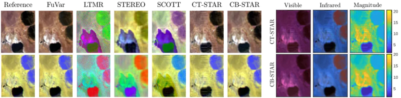
We also evaluate the reconstructed images visually, by displaying true- and pseudo-color representations of the visual and infrared spectra ofZph (corresponding to the wavelengths
0.45, 0.56 and 0.66 µm, and 0.80, 1.50 and 2.20 µm, respectively). Due to space limitations, we only display the results of FuVar, LTMR, STEREO, SCOTT, CT-STAR and CB-STAR, since these are the methods which performed best, and the ones which were conceptually closest to our approach. The spectrally degraded additive factorsP3ppΨq estimated by
CT-STAR and CB-STAR are also evaluated visually, through pseudo-color representations of its visible and infrared spectra, and by the norm (over all bands) of each of its pixels.
Table I
RESULTS-SYNTHETIC EXAMPLE(“RK”STANDS FOR“RANKS”)
Algorithm SAM ERGAS PSNR UIQI time HySure 0.61 19.64 10.85 0.61 5.79 CNMF 0.92 9.03 21.52 0.74 16.3 GLPHS 0.77 4.54 27.44 0.93 7.09 FuVar 0.98 7.85 22.68 0.82 134.2 LTMR 5.69 12.29 18.35 0.71 30.51 STEREO 2.59 12.01 18.44 0.72 0.29 SCOTT 0.58 7.42 22.19 0.89 0.04 CT-STAR, rk:p3, 3, 2q, p2, 2, 1q 0.59 0.73 43.89 1 0.05 CT-STAR, rk:p5, 5, 3q, p3, 3, 2q 0.54 0.63 45.12 1 0.07 CT-STAR, rk:p10, 10, 5q, p5, 5, 3q 0.5 0.59 45.66 1 0.11 CT-STAR, rk:p20, 20, 7q, p7, 7, 3q 1.19 1.29 39.22 1 0.25 CB-STAR, rk:p3, 3, 2q, p2, 2, 1q 0.62 0.78 43.35 1 0.26 CB-STAR, rk:p5, 5, 3q, p3, 3, 2q 0.54 0.63 45.34 1 0.28 CB-STAR, rk:p10, 10, 5q, p5, 5, 3q 0.5 0.55 46.58 1 0.42 CB-STAR, rk:p20, 20, 7q, p7, 7, 3q 1.4 1.47 38.46 0.99 1.08
B. Examples – Synthetic data
To evaluate theproposedalgorithms in a controlled scenario, we first considered a simulation with synthetic data. The tensors Zhand Ψ, of dimensions 100 ˆ 100 ˆ 200, were
gen-erated following the Tucker model, with uniformly distributed entries on the interval r0, 1s and ranks p10, 10, 5q and p5, 5, 3q, respectively. The spectral response function P3P R10ˆ200was
constructed by uniformly averaging groups of 20 bands, and the rest of the simulation setup was the same as described in Section VII-A. For this experiment, we initialized CB-STAR with the results of CT-STAR. We considered two examples. First, we compared the proposed method to other state-of-the-art algorithms, for different choices of rank. Afterwards, we evaluated the sensitivity of CT-STAR and CB-STAR to the presence of additive noise. In both cases, we report average re-sults of a Monte Carlo simulation with 100 noise realizations.
1) Comparison to other algorithms: For this comparison, we set the ranks of STEREO and SCOTT were 50 and p60, 60, 5q, respectively. We also ran the proposed methods with four different rank values (smaller, equal, and larger than the true data ranks), indicated in Table I. The results in Table I show that the proposed methods yielded significant improvements when compared to the other algorithms, which is expected since this dataset was generated according to the model (16)–(17). Moreover, the performance of both CT-STAR
and CB-STAR as a function of the ranks was similar, with the best resultsobservedwhen the rank was the same as the ground truth, but with similar performance when the rank was underestimated. This indicates that CT-STAR and CB-STAR can still perform well when the data rank is higher than the one specified for the model.When the selected rank was over-estimated, the performance of the proposed methods degraded more sharply (with a more prominent decrease for CB-STAR), indicating that the ranks should not be much greater than the true values in order to obtain the best performance.
2) Effect of noise: The exact recovery results obtained in Theorems 2 and 3 assume a noiseless observation model, which is not the case in real applications. To illustrate how the performance of the proposed methods is affected by the presence of additive noise Eh and Em, we evaluated
the quantitative reconstruction metrics for different SNRs, varying from 0dB up to the noiseless case (SNR = 8). For simplicity, we set KZ and KΨas the correct ranks of Zhand
Ψ, respectively. The results are shown in Table II. It can be
seen that the performance of both CT-STAR and CB-STAR decreased for low SNRs. Moreover, CB-STAR achieved better results for high SNRs (ě40dB), but was surpassed by CT-STAR for low SNR scenarios (ď30dB), whose results were considerably better for extremely noisy scenarios (0dB). Moreover, for SNRs found in typical scenes (ě20dB), these results indicate that both methods are able to obtain satisfactory results. Finally, we note that since the ranks of Zh
and Ψ satisfied the requirements of Theorems 2 and 3, exact reconstruction was obtained for SNR = 8 (i.e., the original and reconstructed images were equal up to machine precision). The theoretical results presented in this work made use of two hypotheses to guarantee the recovery of the HRI, namely, that the image and variability factors have low multilinear rank, and that there is no observation noise. However, those hypotheses are often not strictly satisfied in practice. Nonetheless, CT-STAR and CB-STAR only perform a low-rank approximation of the data. Thus, they can still perform well when the true rank of the image is larger than the one specified to the algorithm and under the presence of noise, as illustrated in the previous simulations (even though exact recovery is not guaranteed in those cases). In the following section, we will evaluate the performance of the proposed methods with real HSIs and MSIs, which do not necessarily come from the specified low-rank models.
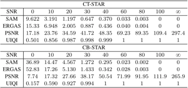
Table II
PERFORMANCE OF THE PROPOSED METHODS FOR DIFFERENTSNRS
CT-STAR SNR 0 10 20 30 40 60 80 100 8 SAM 9.622 3.191 1.197 0.647 0.370 0.033 0.003 0 0 ERGAS 15.33 6.948 2.005 0.887 0.436 0.040 0.004 0 0 PSNR 17.18 23.76 34.59 41.72 48.35 69.23 89.35 109.4 297.4 UIQI 0.501 0.856 0.987 0.998 0.999 1 1 1 1 CB-STAR SNR 0 10 20 30 40 60 80 100 8 SAM 36.89 14.47 4.567 1.272 0.295 0.023 0.002 0 0 ERGAS 52.83 17.26 5.130 1.433 0.342 0.028 0.003 0 0 PSNR 7.74 17.32 27.66 38.17 50.54 71.99 91.95 111.9 265.9 UIQI 0.157 0.590 0.927 0.994 1 1 1 1 1
Lake Isabella Lockwood
Figure 2. Hyperspectral and multispectral images with a small acquisition time difference used in the experiments.
Ivanpah Playa Lake Tahoe A Lake Tahoe B
Figure 3. Hyperspectral and multispectral images with a large acquisition time difference used in the experiments.
C. Example – Real data
In this example, we evaluated the algorithms using real HS and MS images acquired at different time instants, thus presenting different acquisition and seasonal conditions. The reference hyperspectral and multispectral images, with a pixel size of 20 m, acquired by the AVIRIS and by the Sentinel-2A instruments, respectively, were originally considered in [30]. Four sets of image pairs were available. Two of which contained images acquired less than three months apart (thus containing moderate variability). The other two contained images acquired with a time difference of more than one year (thus containing more significant variability). The HSI and MSI contained Lh “ 173 and Lm “ 10 bands, respectively.
The selected ranks for the tensor-based methods are shown in Table III. Although the ranks of CB-STAR satisfied Theorem 3 only for the Ivanpah Playa image pair, this did not have a negative impact on its performance, as will be shown in the following.
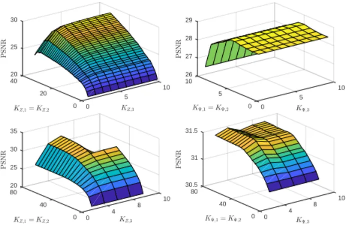
1) Rank sensitivity analysis: Before proceeding, we eval-uate how sensitive the performance of the proposed methods is to the selection of the ranks by plotting the PSNR as a function of each of the ranks KZ,i and KΨ,i, while keeping
the others fixed. For simplicity, we kept the spatial ranks equal to each other (i.e., KZ,1 “ KZ,2 and KΨ,1 “ KΨ,2),
and only show the results for the Lockwood image (to be described in Section VII-C2) due to space limitations4. The
results, shown in Fig. 4, indicate that CT-STAR performs well when KΨ,1 “ KΨ,2 are small, and performs well for values
of KZ,3 which are not small. The optimal KZ,1 “ KZ,2
were relatively large, but a drop in performance was observed when they approach their upper limit Ni´ KΨ,i, i P t1, 2, u.
The performance of CB-STAR increased steadily with KZ,1 “ KZ,2 and for small values of KZ,3, but decreased
more sharply when all values KZ,i, i P t1, 2, 3u were large.
The variability ranks KΨ,i, on the other hand, did not affect the
results too much when KΨ,1“ KΨ,2were sufficiently large.
2) Moderate variability: The first pair of images considered in this example contained 80 ˆ 80 pixels and were acquired over the region surrounding Lake Isabella, on 2018-06-27 and on 2018-08-27. The second pair of images contained 80 ˆ 100
4Additional results are available on the supplemental material.
20 40 25 10 20 30 5 0 0 26 10 27 10 28 5 29 5 0 0 20 80 25 10 30 40 8 35 4 0 0 30.5 80 31 10 40 8 31.5 4 0 0
Figure 4. Sensitivity analysis of the proposed methods Lockwood image. Top: PSNR of CT-STAR as a function of the ranks of Zh(left) and Ψ (right).
Bot-tom: PSNR of CB-STAR as a function of the ranks of Zh(left) and Ψ (right)
Table III
RANKS OF THE TENSOR-BASED ALGORITHMS USED IN THE EXPERIMENTS CT-STAR: CB-STAR: SCOTT: STEREO:
KZ, KΨ KZ, KΨ K K Lockwood p30, 30, 8q, p3, 3, 2q p70, 70, 5q, p40, 40, 3q p60, 60, 5q 50 Lake Isabella p30, 30, 8q, p3, 3, 2q p50, 50, 5q, p40, 40, 3q p60, 60, 5q 50 Lake Tahoe p30, 30, 10q, p3, 3, 1q p35, 35, 9q, p50, 50, 4q p40, 40, 7q 30 Ivanpah Playa p16, 16, 8q, p3, 3, 2q p40, 40, 4q, p40, 40, 5q p30, 30, 30q 10
pixels and was acquired near Lockwood, on 2018-08-20 and on 2018-10-19. A true color representation of the HSI and MSI for this example can be seen in Fig. 2. Due to the relatively small difference between the acquisition dates of both images, the HSI and MSI look similar. However, there are slight differences between them, as seen in the overall color hue of the images and in the upper right part of the Lake Isabella HSI. The quantitative performance metrics of all algorithms are shown in Tables IV and V, while the reconstructed images are presented in Figs.5 and6.
Table IV RESULTS- LOCKWOOD
Algorithm SAM ERGAS PSNR UIQI time HySure 3.38 7.79 23.65 0.88 4.63 CNMF 2.57 5.64 27.6 0.89 8.83 GLPHS 2.57 5.32 28.39 0.91 4.74 FuVar 2.37 4.29 30.59 0.95 218 LTMR 3.47 5.01 29.16 0.94 26.22 STEREO 3.49 5.51 28.72 0.93 1.14 SCOTT 2.52 4.91 29.93 0.95 0.18 CT-STAR 2.96 5.25 28.36 0.92 1.82 CB-STAR, init=interp 2.19 4.35 31.47 0.96 18.8 CB-STAR, init=pseudoinv 2.22 4.34 31.41 0.96 17.98
The quantitative results show that CB-STAR achieved the overall best results for this example, outperforming the other methods in all metrics except in ERGAS, where it performed very similarly to FuVar (which yielded the best results for this metric). CT-STAR, on the other hand, performed similarly to STEREO and SCOTT, being limited by the more stringent constraints on the image ranks. The visual inspection of the results indicates that CB-STAR provides reconstructions
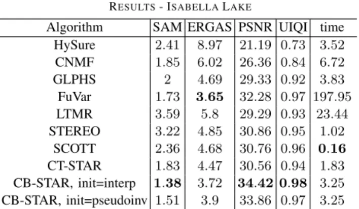
Table V
RESULTS- ISABELLALAKE
Algorithm SAM ERGAS PSNR UIQI time HySure 2.41 8.97 21.19 0.73 3.52 CNMF 1.85 6.02 26.36 0.84 6.72 GLPHS 2 4.69 29.33 0.92 3.83 FuVar 1.73 3.65 32.28 0.97 197.95 LTMR 3.59 5.8 29.29 0.93 23.44 STEREO 3.22 4.85 30.86 0.95 1.02 SCOTT 2.36 4.68 30.76 0.96 0.16 CT-STAR 1.83 4.47 30.56 0.94 1.83 CB-STAR, init=interp 1.38 3.72 34.42 0.98 3.25 CB-STAR, init=pseudoinv 1.51 3.9 33.86 0.97 3.25
closest to the ground truth when compared to the remaining methods. Although FuVar also provided good results, it yielded a slightly worse representation of the road in the left part of the Lockwood HSI, as well as more aberrations in the color of the light-brown regions in the middle of the Isabella Lake scene (which are not seen in the results of CB-STAR).
LTMR, STEREO and SCOTT, not being able to account for variability, yielded slight color aberrations in the reconstruc-tions, which are most clearly seen in the central part of the Isabella Lake image, while CT-STAR produced significant artifacts due to the stringent rank constraints. The estimated factors P3ppΨq are in agreement with the localized changes
observed in Fig.2, particularly in the upper-central area of the Isabella Lake image pair, which is subject to local illumination changes. The computation times of the algorithms show a large difference between that of FuVar and those of the other algorithms, which indicates that CB-STAR achieves better results at a significantly smaller computational complexity.
3) Significant variability: The remaining image pairs used in this example were acquired over the Ivanpah Playa and over Lake Tahoe area. The Ivanpah Playa image pair contained 80ˆ 128 pixels and was acquired on 2015-10-26 and on 2017-12-17. For the Lake Tahoe region, we considered two different im-age pairs (“A” and “B”), both with 100ˆ80 pixels, the first one acquired on 2014-10-04 and on 2017-10-24, and the second one acquired on 2014-09-19 and on 2017-10-24. A true color representation of the HSI and MSI for this example can be seen in Fig.3. Due to the considerable difference between the ac-quisition date/time of the HSI and MSI, significant differences can be found between them. For the Ivanpah Playa images, there are large variations between the sand colors in the central part of the image. For the Lake Tahoe region, significant differences are observed in both image pairs, with differences in the color hues of the ground and of the crop circles for the image pair A, and also a large change in the water level of the lake in the image pair B. The quantitative performance metrics of all algorithms are shown in TablesVI,VII, andVIII, while the reconstructed images are presented in Figs. 7,8 and9.
The quantitative results show that CB-STAR achieved again the overall best results for this example, outperforming the remaining algorithms in most metrics, except in the SAM and UIQI for the Ivanpah Playa HRI and in the SAM of the Lake Tahoe A HRI. Moreover, there was a stronger gap between the performance of the methods that consider variability and the remaining algorithms. CT-STAR, although better thanLTMR,
Table VI RESULTS- IVANPAHPLAYA
Algorithm SAM ERGAS PSNR UIQI time HySure 1.78 4.53 23.35 0.57 6.19 CNMF 1.24 3.22 26.65 0.78 16.36 GLPHS 1.59 3.17 26.84 0.82 5.97 FuVar 1.06 2.04 30.6 0.96 254.97 LTMR 37.25 1,951.53 10.97 0.46 30.53 STEREO 28.17 9,840 20.43 0.61 0.74 SCOTT 35.74 385.28 11.4 0.44 0.21 CT-STAR 1.49 3.44 26.09 0.71 0.18 CB-STAR, init=interp 1.22 1.84 31.56 0.95 71.47 CB-STAR, init=pseudoinv 1.51 2.14 30.3 0.92 48.94 Table VII RESULTS- LAKETAHOEA
Algorithm SAM ERGAS PSNR UIQI time HySure 11.3 13.99 17.37 0.71 4.5 CNMF 8.79 14.59 18.37 0.71 12.1 GLPHS 5.65 7.45 24.08 0.91 4.65 FuVar 3.91 4.73 27.98 0.97 270.91 LTMR 34.45 1,357.42 13.8 0.52 24.94 STEREO 27.07 1,540 20.19 0.68 0.92 SCOTT 33.17 43,100 11.21 0.39 1.47 CT-STAR 5.41 5.25 27.25 0.96 2.88 CB-STAR, init=interp 4.25 3.78 30.1 0.98 63.71 CB-STAR, init=pseudoinv 4.7 3.94 29.67 0.98 31.6 Table VIII RESULTS- LAKETAHOEB
Algorithm SAM ERGAS PSNR UIQI time HySure 7.17 19.08 13.62 0.35 4.36 CNMF 8.08 14.7 16.16 0.42 12.42 GLPHS 3.61 5.58 24.57 0.86 4.53 FuVar 2.58 3.38 28.86 0.96 342.39 LTMR 38.08 1,206.54 12.03 0.46 24.46 STEREO 28.18 6,220 19.99 0.63 0.75 SCOTT 38.45 2,960 10.87 0.31 1.42 CT-STAR 3.07 4.3 26.82 0.92 2.88 CB-STAR, init=interp 2.17 2.64 31.19 0.97 46.46 CB-STAR, init=pseudoinv 2.34 2.73 30.74 0.96 30.08
STEREO and SCOTT, performed significantly worse than CB-STAR due to its stringent constraints on the image ranks. The visual inspection of the results again indicates that CB-STAR provides reconstructions closest to the ground truth when compared to the remaining methods. Although FuVar also provided good results(as it accounts for spectral variability), the reconstructions by CB-STAR were closer to the ground truth, as can be observed in the color shades of the upper part of the Ivanpah Playa image and of the crop circles of the Lake Tahoe A image, and especially in the overall colors in the more uniform regions containing soil and water and vegetation in the Lake Tahoe B image. However, FuVar results showed slightly sharper edges in some regions (e.g., around the crop circles in the Lake Tahoe images), which occurs due to the use of a Total Variation spatial regularization. Nonetheless, a spatial regularization can also be incorporated to the CB-STAR cost function in (53) to achieve a similar effect. LTMR,