HAL Id: hal-01462213
https://hal.inria.fr/hal-01462213
Submitted on 8 Feb 2017
HAL is a multi-disciplinary open access
archive for the deposit and dissemination of
sci-entific research documents, whether they are
pub-lished or not. The documents may come from
teaching and research institutions in France or
L’archive ouverte pluridisciplinaire HAL, est
destinée au dépôt et à la diffusion de documents
scientifiques de niveau recherche, publiés ou non,
émanant des établissements d’enseignement et de
recherche français ou étrangers, des laboratoires
Loris Marchal, Samuel Mccauley, Bertrand Simon, Frédéric Vivien
To cite this version:
Loris Marchal, Samuel Mccauley, Bertrand Simon, Frédéric Vivien. Minimizing I/Os in Out-of-Core
Task Tree Scheduling. [Research Report] RR-9025, INRIA. 2017. �hal-01462213�
0249-6399 ISRN INRIA/RR--9025--FR+ENG
RESEARCH
REPORT
N° 9025
February 2017Out-of-Core Task Tree
Scheduling
RESEARCH CENTRE GRENOBLE – RHÔNE-ALPES Inovallée
Loris Marchal, Samuel McCauley, Bertrand Simon, Frédéric
Vivien
Project-Team ROMA
Research Report n° 9025 — February 2017 — 24 pages
Abstract: Scientific applications are usually described as directed acyclic graphs, where nodes repre-sent tasks and edges reprerepre-sent dependencies between tasks. For some applications, such as the mul-tifrontal method of sparse matrix factorization, this graph is a tree: each task produces a single output data, used by a single task (its parent in the tree).
We focus on the case when the data manipulated by tasks have a large size, which is especially the case in the multifrontal method. To process a task, both its inputs and its output must fit in the main memory. Moreover, output results of tasks have to be stored between their production and their use by the parent task. It may therefore happen, during an execution, that not all data fit together in memory. In particular, this is the case if the total available memory is smaller than the minimum memory required to process the whole tree. In such a case, some data have to be temporarily written to disk and read afterwards. These Input/Output (I/O) operations are very expensive; hence, the need to minimize them.
We revisit this open problem in this paper. Specifically, our goal is to minimize the total volume of I/O while processing a given task tree. We first formalize and generalize known results, then prove that existing solutions can be arbitrarily worse than optimal. Finally, we propose a novel heuristic algorithm, based on the optimal tree traversal for memory minimization. We demonstrate good performance of this new heuristic through simulations on both synthetic trees and realistic trees built from actual sparse matrices.
Résumé : Les applications de calcul scientifique sont souvent décrites comme des graphes de tâches dirigés et acycliques, où les nœuds représentent les tâches et les arêtes représentent les dépendances entre tâches. Pour certaines applications, comme les méthodes multifrontales de factorisation de ma-trices creuses, le graphe correspondant est un arbre: chaque tâche produit un unique fichier de don-nées en sortie qui est utilisé par une unique tâche (son père dans l’arbre).
On s’intéresse ici dans le cas où les fichiers de données manipulés par les tâches sont de grande taille, ce qui est en particulier le cas dans les méthodes multifrontales. Pour traiter une tâche, ses fichiers d’entrée et de sortie doivent se trouver dans la mémoire principale. De plus, les fichiers de sortie doivent être stockés entre leur création et leur utilisation par la tâche père. Il peut donc arriver que, durant une exécution, la mémoire disponible soit inférieure à la mémoire minimum requise pour traiter l’arbre complet. Dans ce cas, certaines données doivent être temporairement transférées sur un disque pour être lues ultérieurement. Ces opérations d’Entrées/Sorties (E/S ou I/O en anglais) sont très coûteuses, d’où le besoin de les minimiser.
Nous revisitons dans cet article ce problème ouvert. Plus précisément, notre objectif est de mi-nimiser le volume total d’Entrées/Sorties effectuées en traitant un arbre de tâche donné. Nous com-mençons par formaliser et généraliser des résultats connus, puis nous prouvons que les solutions exis-tantes peuvent être arbitrairement loin de l’optimal. Finalement, nous proposons une nouvelle heu-ristique, basée sur le parcours d’arbre minimisant l’utilisation mémoire. Nous établissons les bonnes performances de cette heuristique à travers des simulations sur des arbres synthétiques ainsi que des arbres réalistes construits à partir de matrices creuses réelles.
1 Introduction
Parallel workloads are often modeled as task graphs, where nodes represent tasks and edges represent the dependencies between tasks. There is an abundant literature on task graph scheduling when the objective is to minimize the total completion time, or makespan. However, with the increase of the size of the data to be processed, the memory footprint of the application can have a dramatic impact on the algorithm execution time, and thus needs to be optimized. When handling very large data, the available main memory may be too small to simultaneously handle all data needed by the computa-tion. In this case, we have to resort to using disk as a secondary storage, which is sometimes known as
out-of-core execution. The cost of the I/O operation to transfer data from and to the disk is known to
be several orders of magnitude larger than the cost of accessing the main memory. Thus, in the case of out-of-core execution, it is a natural objective to minimize the total volume of I/O.
In the present paper, we consider the parallel scheduling of rooted in-trees. The vertices of the trees represent computational tasks, and the edges of the trees represent the dependencies between these tasks. Tasks are defined by their input and output data. Each task uses all the data produced by its children to output new data for its parent. In particular, a task must have enough available memory to fit the input from all its children.
The motivation for this work comes from numerical linear algebra, and especially the factorization of sparse matrices using direct multifrontal methods [1]. During the factorization, the computations are organized as a tree workflow called an elimination tree, and the huge size of the data involved makes it absolutely necessary to reduce the memory requirement of the factorization. Note that we consider here that no numerical pivoting is performed during the factorization, and thus that the structure of the tree, as well as the size of the data, are known before the computation really happens. It is known that the problem of minimizing the peak memory Mpeakof a tree traversal, that is, the
minimum amount of memory needed to process a tree, is polynomial [2, 3]. However, it may well happen that the available amount of memory M is smaller than the peak memory Mpeak. In this case,
we have to decide which data, or part of data, have to be written to disk. In a previous study [3], we have focused on the case when the data cannot be partially written to disk, and we proved that this variant of the problem was NP-complete. However, it is usually possible to split data that reside in memory, and write only part of it to the disk if needed. This is for instance what is done using paging: all data are divided in same-size pages, which can be moved from main memory to secondary storage when needed. Since all modern computer systems implement paging, it is natural to consider it when minimizing the I/O volume.
Note that as in [3], the present study does not directly focus on parallel algorithms. However, paral-lel processing is the ultimate motivation for this work: complex scientific applications using large data such as multifrontal sparse matrix factorization always make use of parallel platforms. Most involved scheduling schemes combine data parallelism (a task uses multiple processors) and tree parallelism (several tasks are processed in parallel). We indeed have studied such a problem for peak memory minimization [4]. However, one cannot hope to achieve good results for the minimization of I/O vol-ume in a parallel settings until the sequential problem is well understood, which is not yet the case. The present paper is therefore a step towards understanding the sequential version of this problem.
The main contributions of this work are:
• A formalization in a common framework of the results scattered in the literature;
• A proof of the dominance of post-order traversals when trees are homogeneous (all output data have the same size), knowing that an algorithm to compute the best post-order traversal has been proposed by E. Agullo [5].
• A proof that neither the best post-order traversal nor the memory-peak minimization algo-rithms are approximation algoalgo-rithms for minimizing the I/O volume;
• A new heuristic that achieves good performance both on synthetic and actual trees as shown through simulations.
The rest of this paper is organized as follows. We give an overview of the related work in Section 2. Then in Section 3 we formalize our model and present elementary results. Existing solutions are stud-ied in Section 4 before a new one is introduced in Section 5 and evaluated through simulations in Section 6. We finally conclude and present future directions in Section 7.
2 Related work
Memory and storage have always been a limited parameter for large computations, as outlined by the pioneering work of Sethi and Ullman [6] on register allocation for task trees. In the realm of sparse direct solvers, the problem of scheduling a tree so as to minimize peak memory has first been investi-gated by Liu [7] in the sequential case: he proposed an algorithm to find a peak-memory minimizing traversal of a task tree when the traversal is required to correspond to a postorder traversal of the tree. A postorder traversal requires that each subtree of a given node must be fully processed before the processing of another subtree can begin. A follow-up study [2] presents an optimal algorithm to solve the general problem, without the postorder constraint on the traversal. Postorder traversals are known to be arbitrarily worse than optimal traversals for memory minimization [3]. However, they are very natural and straightforward solutions to this problem, as they allow to fully process one subtree be-fore starting a new one. Therebe-fore, they are widely used in sparse matrix software likeMUMPS[8, 9], and achieve good performance on actual elimination trees [3]. Note that peak memory minimization is still a crucial question for direct solvers, as highlighted by Agullo et al. [10], who study the effect of processor mapping on memory consumption for multifrontal methods.
As mentioned in the introduction, the problem of minimizing the I/O volume has been studied in [3] with the constraint that each data either stays in the memory or has to be written wholly to disk. We study here the case when we have the option to store part of the data, which is also the topic of E. Agullo’s PhD. thesis [5]. In his thesis, Agullo exhibits the best postorder traversal for the minimization of the I/O volume, which we adapt to our model in Section 4.1. He also studies numerous variants of the model that are important for direct solvers, as well as other memory management issues—both for sequential and parallel processing. Based on these preliminaries, he finally presents an out-of-core version of the MUMPS solver.
Finally, out-of-core execution is a well-know approach for computing on large data, especially (but not only) in linear algebra [11, 12].
3 Problem modeling and basic results
3.1 Model and notation
As introduced above, we assume that we have an available memory (or primary storage) of limited size M , and a disk (or secondary storage) of unlimited size.
We consider a workflow of tasks whose precedence constraints are modeled by a tree of tasks G = (V, E ). Its nodes v ∈ V represent tasks and its edges e ∈ E represent dependencies. All dependencies are directed toward the root (denoted by root): a node can only be executed after the termination of all its children. The output data of a node i occupies a size wi in the main memory. This data may
be written totally or partially to the disk after task i produces it. In order for a node to be executed, the output data of all its children must be entirely stored in the main memory. An amount of memory
m can be moved between the memory and the disk at a cost of m I/O operations, regardless of which
(such as kilobytes) and are integers. We divide the main memory into slots, where each slot holds one such unit of memory.
At the beginning of the computation of a task i , the output data of i ’s children must be in memory, while at the end of its computation, its own output data must be in memory. The amount of memory needed in order to execute node i is thus
¯ wi= max à wi, X ( j ,i )∈E wj ! .
We assume that M is at least as large as every ¯wi, as otherwise the tree cannot be processed.
Our objective is to find a solution minimizing the total I/O volume. A solution needs to give the order in which nodes should be executed, and how much of each node should be written out during I/O operations. In particular, for a tree of n tasks, we define a solution to our problem as a permutation
σ of [1...n] and a function τ. We call such a solution a traversal. The permutation σ represents the schedule of the nodes, that is,σ(i) = t means that task i is computed at step t, while the function τ
represents the amount of I/O for each data:τ(i) = m means that m among wiunits of the output data
of task i are written to disk (then we assume they are written as soon as task i completes). Note that we do not need to clarify which part of the data is written to disk, as our cost function only depends on the volume. Besides, we assume that whenτ(i) 6= 0, the write operation on the output data of task i is performed right after task i completes (and produces the data), and the read operation is performed just before the use of this data by task i ’s parent, as any other I/O scheme would use more memory at some time step for the same I/O volume. Finally, since there are as many read than write operations, we only count the write operations.
In order for a traversal to be valid, it must respect the following conditions: • Tasks are processed in a topological order:
∀(i , j ) ∈ E , σ(i ) < σ( j );
We say that a node i of parent j is considered active at step t under the scheduleσ if σ(i) < t <
σ(j). This means that its output data is either partially in memory and/or partially written to
disk at time t .
• The amount of data written to disk never exceeds the size of the data: ∀i ∈ V, 0 ≤ τ(i ) ≤ wi;
• Enough memory remains available for the processing of each task (taking into account active nodes):
∀i ∈ G, X
(k,p)∈E
σ(k)<σ(i)<σ(p)
(wk− τ(k)) ≤ M − ¯wi.
The problem we are considering in this paper, called MINIO, is to find a valid traversal that mini-mizes the total amount of I/O, given byP
i ∈Gτ(i).
We formally define a postorder traversal as a traversalσ such that, for any node i and for any node
k outside the subtree Tirooted at i , we have either ∀j ∈ Ti,σ(k) < σ(j) or ∀j ∈ Ti,σ(j) < σ(k).
3.2 Towards a compact solution
Although a traversal is described by both the scheduleσ and the I/O function τ, the following results show that one can be deduced from the other. The first result is adapted from [5, Property 2.1], which has the same result limited to postorder traversals (see Section 2). It states that given a scheduleσ, it is easy to derive a I/O schemeτ which minimizes the I/O volume of the traversal (σ,τ).
Theorem 1. We consider a tree G, a memory bound M , and a scheduleσ. The I/O function τ following
the Furthest in the Future policy achieves the best performance underσ.
The I/O functionτ following the Furthest in the Future (FiF) policy is defined as follows: during the execution ofσ, whenever the memory exceeds the limit M, I/O operations are performed on the active nodes which will remain active the furthest in the future, i.e., whose execution come last in the scheduleσ. This result is similar to Belady’s rule which states the optimality of the offline MIN cache replacement [13, 14], that evicts from the cache the data which is used the latest.
Proof. Given a tree G, a memory bound M , a scheduleσ and a I/O function τ that does not respect the
FiF policy, it is straightforward to transformτ into another I/O function τ0following the rule. Consider
the first step when an I/O is performed on a data i that is not the last one to be used among active data. Let j denote the last data used among active ones. We can safely increaseτ0( j ) and decreaseτ0(i ) until
eitherτ0( j ) = wj orτ0(i ) = 0. As j is active longer than i is, the memory freed by τ0is available for a
longer time than the one freed byτ, which keeps the traversal valid. Furthermore, by repeating this transformation, we produce an I/O function which respects the FiF policy.
On the other hand, if we have an I/O functionτ describing how much of each node is written to disk, we can compute a scheduleσ such that (σ,τ) is a valid traversal (if such a schedule exists). Theorem 2. We consider a tree G, a memory bound M , and an I/O functionτ for which there exists a
valid schedule. Such a schedule can be computed in polynomial time.
The proof of this result is delegated to Section 5 where we use a similar method to derive a heuris-tic: once we know where the I/O operations take place, we may transform the tree by expanding some
nodes to make these I/O operations explicit within the tree structure. If a valid traversal usingτ exists,
the resulting tree may be completely scheduled without any additional I/O, and such a schedule can be computed using an optimal scheduling algorithm for memory minimization.
Both previous results allow us to describe solutions in a more compact format (as either a schedule or an I/O function). However, this does make the problem less combinatorial: there are n! possible schedules and already 2nτ functions if we restrict only to functions such that τ(i) = 0 or wi.
3.3 Related algorithms
As mentioned in Section 2, the problem of minimizing the peak memory, denoted MINMEM, is strongly related to our problem, and has been extensively studied. In this problem, the available mem-ory is unbounded (which means no I/Os are required) and we look for a schedule that minimizes the peak memory, i.e., the maximal amount of memory used at any time during the execution. There are at least two important algorithms for this problem, which we use in the present paper:
• It is possible to compute a schedule minimizing the peak-memory in polynomial time, as proved by Liu [2]. We denote such an algorithm by OPTMINMEM.
• The best postorder traversal for peak-memory minimization can also be computed in polyno-mial time [7]. We will refer to this algorithm by POSTORDERMINMEM.
4 Existing solutions are not satisfactory
We now detail two existing solutions for the MINIO problem. The first one is the best postorder traver-sal proposed by Agullo [5]. The second consists in using the optimal travertraver-sal for MINMEMproposed by Liu [2] and then to apply Theorem 1 to obtain a valid traversal. After presenting these algorithms, we prove that none of them has a constant competitive factor compared to the optimal traversal.
4.1 Computing the best postorder traversal
For the sake of completeness, we present the adaption to our model of the algorithm computing the best postorder traversal for MINIO from [5]. Recall that in a postorder traversal, when a node is
pro-cessed, its whole subtree must be processed before any other external node may be started. Given a node i and a postorder scheduleσ, we first recursively define Si as the storage requirement of the
subtree Ti rooted at i . Let Chil(i ) be the children of i . Then:
Si= max wi, max j ∈Chil(i ) Sj+ X k∈Chil(i ) σ(k)<σ(j) wk .
This expression represents the maximum memory peak reached during the execution. If the peak is obtained at the end of the execution, it is then equal to wi. Otherwise, it appears during the execution
of the subtree of some child j . In this case, the peak is composed of the weights of the children already processed, plus the peak Sjof Tj.
We may now consider Ai= min(M, Si), which represents the amount of main memory used for the
out-of-core execution of the subtree Tibyσ. We recursively define Vias the volume of I/Os performed
byσ during the execution Tiwhen I/O operations are done using the FiF policy:
Vi= max à 0, max j ∈Chil(i ) à Aj+ σ(k)<σ(j) X k∈Chil(i ) wk ! − M ! + X j ∈Chil(i ) Vj.
The expression of Vihas a similar structure to the expression of Si. No I/Os can be incurred when only
the root i is in memory, hence wihas no effect here. The second term accounts for the I/Os incurred
on the children of i . Indeed, during the execution of node j , some parts of children of i must be written to disk if the memory peak exceeds M , and this quantity is at least Aj+Pσ(k)<σ(j)k∈Chil(i ) wk− M. The
last term accounts for the I/Os occurring inside the subtrees. Note that such I/Os can only happen if the memory peak of the subtree exceeds M .
It remains to determine which postorder traversal minimizes the quantity Vroot. Note that the only
term sensitive to the ordering of the children of i in the expression of Vi is max j ∈Chil(i ) Ã Aj+ σ(k)<σ(j) X k∈Chil(i ) wk ! . Theorem 3 states that sorting the children of i by decreasing values of Aj− wj achieves the minimum
Vi.
Theorem 3 (Lemma 3.1 in [7]). Given a set of values (xi, yi)1≤i ≤n, the minimum value of
max1≤i ≤n³xi+Pi −1j =1yj
´
is obtained by sorting the sequence (xi, yi) in decreasing order of xi− yi.
Therefore, the postorder traversal that processes the children nodes by decreasing order of Ai−wi
minimizes the I/O cost among all postorder traversals. This traversal is described in Algorithm 1, initially called with r = root, and will be referred to as POSTORDERMINIO. Note that in the algorithm ⊕ refers to the concatenation operation on lists.
4.2
P
OSTO
RDERM
INIO is optimal on homogeneous trees
In this section we focus on homogeneous trees, that is on trees where all nodes have output data of size one. We will show that POSTORDERMINIO is optimal on these homogeneous trees, i.e., that it performs the minimum number of I/Os. This generalizes a result of Sethi and Ullman [6] for homoge-neous binary trees.
Algorithm 1: POSTORDERMINIO (G, r ) Output: a tree G and a node r in G
Output: an ordered list`r of the nodes in the subtree rooted at r , corresponding to a postorder
1 foreach i child of r do
2 `i← POSTORDERMINIO(G, i )
3 Compute the Aivalue using postorder`i
4 `r← ;
5 for i child of r by decreasing value of Ai− wido
6 `r← `r⊕ `i
7 `r← `r⊕ {r }
8 return`r
Theorem 4. POSTORDERMINIO is optimal for homogeneous trees.
In order to prove this theorem, we need first to define some labels on the nodes of a tree. Let T be any homogeneous tree (wv= 1 for all nodes v of T ). In the following definitions, whenever v is a node
of T with k children, v1, . . . , vkwill be its children.
Memory bound l (v). For each node v of T , we recursively define a label l (v) which represents the minimum amount of memory necessary to execute the subtree T (v) rooted at v without per-forming any I/Os:
l (v) = 0 if v is a leaf
max1≤i ≤k(l (vi) + i − 1) otherwise
and ordering the children such that
l (vi) ≥ l (vi +1) for 1 ≤ i ≤ k − 1
We call POSTORDER one postorder schedule that executes the children of any node by non-increasing l -labels (ties being arbitrarily broken). Intuitively, under POSTORDER, while comput-ing the i -th child, we have i −1 extra nodes in memory, each of size one, so we need l (vi)+(i −1)
memory slots in total.
I/O indicator c(v). If vi is a child of v, intuitively, c(vi) represents the number of children of v written
to disk by POSTORDERduring the execution of T (vi). This number can be either 0 or 1. We set
c(v1) = 0 and
c(vi) =
½
0 if l (vi) +P1≤j <i(1 − c(vj)) ≤ M
1 otherwise.
We set c(root) = 0 where root is the root of T . To ease the writing of some proofs, we use the notation
m(vi) =
X
1≤j <i
(1 − c(vj)).
Thus m(vi) represents the number of children of v in memory when vi is executed. Note that
m(v1) = 0 and m(vi) = (1 − c(v1)) +P2≤j <i(1 − c(vj)) ≥ (1 − c(v1)) = 1 for 2 ≤ i ≤ k.
I/O volumes w (v) and W (T (v)). w (v) represents the total number of children of v stored by POS
-TORDER: w (v) = k X i =1 c(vi) = k X i =2 c(vi).
Finally, for a given node v, we define W (T (v)) on the subtree rooted at v:
W (T (v)) = c(v) + X
µ∈T (v)
w (µ).
W (T (v)) intuitively represents the total volume of communications performed during the
exe-cution of the tree T (v) by POSTORDER.
We first state the correctness of the l -labels and the optimality of POSTORDERfor the MINMEM
problem.
Lemma 1. With infinite memory, POSTORDERuses l (n) slots to compute the subtree rooted at node n.
Proof. This result follows from the definition of the labels l (v).
Lemma 2. With infinite memory, any schedule uses at least l (v) slots to compute the subtree rooted at
v.
Proof. We prove this result by induction on the size of T (v). If v is a leaf, the result holds (l (v) = 1).
Otherwise, we assume the lemma to be true for the subtrees rooted at the children v1, . . . , vk of
v. We consider the schedule returned by MINMEM. The memory peak inherent to the execution of a subtree T (vi) is equal to l (vi) by the induction hypothesis. Assume without loss of generality that the
children of v are ordered such that MINMEMfirst computes a node of T (v1), then the next executed
node not in T (v1) is in T (v2), then the next executed node neither in T (v1) nor in T (v2) is in T (v3), and
so on. Then, the memory peak reached during the execution of T (vi) is at least l (vi) + (i − 1) because,
in addition to T (vi), at least i − 1 subtrees have been partially executed: T (v1), ..., T (vi −1). Finally, the
total memory peak is at least equal to max1≤i ≤k(l (vi)+i −1). By Theorem 3, this quantity is minimized
when the nodes are ordered by non-increasing values of l (vi). Hence, the total memory peak is at least
l (v).
We now state the performance of POSTORDERfor the MINIO problem (I/Os are done following the FiF policy).
Lemma 3. POSTORDERcomputes a given tree T using at most W (T ) I/Os.
Proof. We prove this result by induction on the size of T . We introduce a new notation: for any node v of T we defineW (v) as W (v) = W (T (v)) − c(v). In other words, W (v) represents the total volume of
communications performed during the execution of the tree T (v) if we had nothing to execute but
T (v) (in practice T (v) may be a strict sub-tree of T and, therefore, the execution of T (v) in the midst
of the execution of T can induce more communications). Note thatW (v) = W (T (v)) if v is the root of
T . We prove by induction on the size of T (v) that POSTORDERperforms at mostW (v) I/Os during the execution of T (v) if POSTORDERhas nothing to execute but T (v).
Let us assume that v is a leaf. Because we have assumed (in Section 3.1) that M was large enough for a single node to be processed without I/Os, c(v) = 0 and thus W (T (v)) = 0 = W (v) + c(v). On the other hand, POSTORDERperforms 0 I/O during the execution of T (v).
Now assume that v is not a leaf. By the induction hypothesis, for any i ∈ [1;k], POSTORDERexecutes the tree T (vi) alone using at mostW (vi) I/Os. We prove that to process the tree T (vi), after the trees
T (v1) through T (vi −1) were processed, we need to perform at most W (T (vi)) = W (vi) + c(vi) I/Os.
Let us consider the (i + 1)-th child of v. If c(vi +1) = 0, then l (vi +1) +P1≤j <i +1(1 − c(vj)) ≤ M.
Then, according to Lemma 1, no I/Os are required to execute T (vi +1) under POSTORDEReven after the processing of T (v1) through T (vi). Indeed, before the start of the processing of T (vi +1) the memory
contains exactlyP
1≤j <i +1(1−c(vj)) nodes. ThereforeW (vi +1) = c(vi +1) = W (T (vi +1)) = 0 and we have
We are now in the case c(vi +1) = 1; thus l (vi +1) +P1≤j <i +1(1 − c(vj)) > M. Recall that for l ∈ [1;i ],
l (vl) ≥ l (vi +1). Thus, if l (vi +1) ≥ M, then for l ∈ [2;i ], l (vl) ≥ M and c(vl) = 1 (because m(vl) ≥ (1 −
c(v1)) = 1). Therefore, after the completion of T (vi) there is only one node remaining in the memory:
vi. Then using a single I/O POSTORDERwrites vito disk, the memory is empty, and T (vi +1) can then
be processed withW (vi +1) I/Os, giving a total of at mostW (vi +1) + c(vi +1) = W (T (vi +1)) I/Os. The
only remaining case is the case l (vi +1) < M. The processing of T (vi) requires at least l (vi +1) empty
memory slots because l (vi) ≥ l (vi +1). Hence, after the completion of T (vi) there are at least l (vi +1)−1
empty memory slots (the memory including the node vi itself ). Then using a single I/O POSTORDER
writes vito disk and there are enough empty memory slots to process T (vi +1) without any additional
I/Os. Therefore we need to perform at most W (T (vi +1)) = W (vi +1) + c(vi +1) I/Os. This concludes the
proof.
Lemma 5 relies on the following intermediate result.
Lemma 4. Consider a node v of a tree T with a child, a, whose label l (a) satisfies l (a) > M. Now,
consider any tree T0 identical to T , except that the subtree rooted at a has been replaced by any tree whose new label l0(a) satisfies l (a) ≥ l0(a) ≥ M. Then w0(v) = w(v).
Proof. Let v1, . . . , vkbe the children of v, ordered so that l (v1) ≥ ··· ≥ l (vk). Let j be the index of a:
a = vj. As the label of a in T0, l0(a), is not larger than l (a), we can have l0(a) < l0(vj +1). Therefore, we
define another ordering of the children of v denoted by v0
1, . . . , v0ksuch that l0(v10) ≥ ··· ≥ l0(v0k). Let j0
be the index of a in this ordering: v0
j0= a = vj.
Note that j0≥ j . For i ∈ [ j + 1; j0], we have v
i = vi −10 ; at j , we have vj= v0j0; and for i ∉ [ j ; j0], we
have vi= v0i.
If j0= 1 then j = 1. This case means that a remains the node with the largest label. The labels of
the other children of v remain unchanged. Because c(v1) = c0(v1) = 0 by definition, then c0(vi) = c(vi)
for any child viof v and, thus, w (v) is equal to w0(v).
Let us now consider the case j0> 1. From what precedes, v0j0
−1= vj0. Then l (vj0) = l 0(v0
j0−1) ≥
l0(v0
j0) = l0(a) ≥ M. However, for any i ∈ [1; j0], l0(v0i) ≥ l0(v0j0) ≥ M and l (vi) ≥ l (vj0) ≥ M. Therefore,
for any i ∈ [2; j0], l0(v0
i) + m0(vi0) > M (because m0(vi0) ≥ 1 − c0(v01) = 1 ) and, thus, c0(v0i) = 1. Similarly,
for any i ∈ [2; j0], l (v
i) + m(vi) > M (because m(vi) ≥ m(v1) = 1 ) and, thus, c(vi) = 1. Therefore, for
i ∈ [1; j0], c(v
i) = c0(vi0). Then, for i ∈ [ j0+1; k], vi= v0i, m(vi) = m0(vi0), and c(vi) = c0(v0i) by an obvious
induction. Therefore, w0(v) =Pk
i =2c0(v0i) =
Pk
i =2c(vi) = w(v).
The following lemma gives a lower bound on the I/Os performed by any schedule. Lemma 5. No schedule can compute a tree T performing strictly less than W (T ) I/Os.
Proof. We proceed by induction on the number of nodes of T .
The base case consists of a tree T that can be scheduled without any I/O. For contradiction, assume that W (T ) > 0. Then there exists a node v of T such that w(v) > 0 and a child viof v such that c(vi) = 1.
Then, by definition of c(vi) and of l (v), l (v) > M. However, according to Lemma 2, “any schedule uses
at least l (v) slots to compute T (v)”, so T (v), and thus T , cannot be scheduled without I/Os. Hence, a contradiction; thus W (T ) = 0.
Consider a tree T that cannot be scheduled without I/Os, and a schedule P on T that minimizes the total volume of I/Os.
First, by Lemma 1, there exists a node v such that l (v) > M. Otherwise, POSTORDERwould be able to schedule T without I/Os, which would violate our assumption on T . Then, the label of the root r of
T also satisfies l (r ) > M.
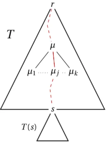
Let s be the first node to be stored under P . Then, the subtree T (s) has been scheduled without I/Os so, by Lemma 2, we have l (s) ≤ M and, hence, no node of T (s) has a label larger than M. Let
s r µ
T
T (s) µ1 µj µkFigure 1: Scheme of the composition of the tree T .
µ be the closest ancestor of s to have a label larger than M. µ exists as l(r ) > M and l(s) ≤ M. Let µ1, . . . ,µkbe the children ofµ, ordered such that l(µi) ≥ l (µi +1). Let j be such thatµjis either s or one
of its ancestors. Let t = min{i ∈ [1;k] | l (µi) + i − 1 > M} (t exists because, by definition, l (µ) > M). See
Figure 1 for an illustration of the tree.
Let T0be the tree obtained from T by replacing s by a leaf, therefore replacing the subtree T (s) by a single node s. As T (s) cannot be empty, T0contains fewer nodes than T . Consider a schedule P0on
T0that executes the same operations as P on T and in the same order, except for the ones concerning
T (s).
We use the following notation: as above, l , m, c, w are defined on nodes of the tree T , whereas l0, m0, c0, w0refer to the same values on the tree T0. The nodes in T0share the same names as their equiv-alent in T .
We define, as in the proof of Lemma 4, an orderingµ01, . . . ,µ0kon the children ofµ, l0(µ0i) ≥ l0(µ0i +1). Furthermore, we assume that this order is consistent with the original one, which means the following. Let j0be such thatµj = µ0j0. Note that j0≥ j . For i ∈ [ j + 1; j0], we haveµi = µ0i −1; at j ,µj = µ0j0; for
i ∉ [j ; j0], we haveµ
i= µ0i. In particular, we haveµj0= µ0
j0−1if j0> j and µj0= µ0
j0if j0= j .
Note that, except s and its ancestors, every node v of T0satisfies l (v) = l0(v) and w (v) = w0(v). Our objective is to prove that W (T0) ≥ W (T ) − 1. We first prove that l0(µ) ≥ M. We split into cases based on the value of t defined above:
1. t < j . The labels of µ1, . . . ,µtare left unchanged so l0(µ) ≥ l0(µt) + t − 1 > M.
2. t = j . By definition of µ, we have l (µj) ≤ M, so we cannot have t = j = 1. The labels of µ1, . . . ,µt −1
are left unchanged, and l (µt −1) ≥ l (µt), so
l0(µ) ≥ l0(µt −1) + t − 2 ≥ l (µt) + t − 1 − 1 > M − 1.
3. t > j . Among µ1, . . . ,µt, the only label that changed isµj. Therefore there are t − 2 nodes that
have a label l0larger than that ofµ
t. Hence,
l0(µ) ≥ l0(µt) + t − 2 > M − 1.
Now, we prove that w0(µ) ≥ w(µ) − 1, by showing that there exists at most one index i such that c(µi) = 1 and c0(µi) = 0. Let I be the set of such indexes. Note that no index strictly smaller than j can
be in I as the relevant labels are identical in both trees.
1. c(µj) = 0. Thus j ∉ I . Let a = min{i ∈ [ j + 1,k] | c(µi) = 1}. There are several cases; in each we
show that I contains at most one element. (a) First, a does not exist. Then I is empty.
(b) Assume a > j0. No index in [1; j ] can be in I , and thus no index in [1; j0]. In particular,
c(vl) = 0 for l ∈ [ j ; j0] by definition of a. Because nodeµj appears right after nodeµj0
in T0, then m0(µj) = m0(µj0) + (1 − c(µj0)) = (m(µj0) − (1 − c(µj))) + (1 − c(µj0)) = m(µj0) +
c(µj) − c(µj0) = m(µj0). Therefore, we have m0(µj) = m(µj0). As l0(µj) ≤ l0(µj0), we get
m0(µj) + l0(µj) ≤ m(µj0) + l0(µj0). Then, because l0(µj0) = l (µj0), and by the definition of c,
we conclude that c0(µj) ≤ c(µj0).
By definition, j0≥ j . Because a > j0, if j0> j , then c(µj0) = 0 by definition of a.
Other-wise j0= j and we use the assumption c(µj) = 0 to conclude that in all cases c(µj0) = 0.
Combined with c0(µj) ≤ c(µj0) this gives us c0(µj) = 0.
Recall that the labels in [1; j − 1] are left unchanged, so c(µi) = c0(µi) for i ∈ [1; j − 1]. From
what precedes, c0(µj) = c(µj) = 0. By definition of a and because j0< a, c(µi) = 0 for
i ∈ [j + 1; j0]. Thus, all these nodes have the same label l in T0and T , and all of them have m0(µ
i) ≤ m(µi) (by definition of m: they are preceded by the same nodes so their sums
have the same terms, except nodeµj). Therefore, for all these nodes c0(µi) = 0 and thus
c0(µ
i) = c(µi). Hence, m(µj0+1) = m0(µj0+1). Because l (µj0+1) = l0(µj0+1) we conclude that
c(µj0+1) = c0(µj0+1). We then proceed by a simple induction on the nodes with a larger
index to prove that I is empty.
(c) Now, assume a ≤ j0. Once again, because the labels in [1; j − 1] are left unchanged, and because c(µj) = 0, no index in [1; j ] can be in I , and thus no index in [1; a − 1] can be in I .
We have two cases to consider, depending on whether a is equal to 2 (recall that by defini-tion a ≥ j + 1 ≥ 2).
i. a = 2. Then j = 1. Therefore, in T0,µais the first child and, by definition of c, c0(µa) =
0.
ii. a > 2. By definition of a, c(µa) = 1. Then, either a = j + 1 and then a − 1 = j and
c(µa−1) = c(µj) = 0, or a > j + 1 and then c(µa−1) = 0 by definition of a. In all
cases, c(µa−1) = 0. Therefore, l (µa−1) + m(µa−1) ≤ M. Because l (µa−1) ≥ l (µa) and
m(µa) = m(µa−1) + 1, l (µa) + m(µa) ≤ M + 1. Because c(µa) = 1 by definition of a,
l (µa) = m(µa) ≤ M + 1.
Recall (for the third time) that the labels in [1; j −1] are left unchanged, so c(µi) = c0(µi)
for i ∈ [1; j −1]. Moreover, by definition of a, c(µi) = 0 for all i ∈ [ j +1; a −1]. Therefore,
because c(µj) = 0, for all i ∈ [ j + 1; a − 1] m0(µi) = m(µi) − 1 and thus c0(µi) = c(µi) = 0.
Also, m0(µ
a) = m(µa) − 1. Then l0(µa) + m0(µa) = l (µa) + m(µa) − 1 = M from what
precedes. Therefore, c0(µ
a) = 0.
Because c0(µa) = 0, m0(µa+1) = m(µa+1). Then, by an immediate induction, m0(µi) = m(µi)
for i ∈ [a + 1; j0]. Therefore [a + 1; j0] ∩ I = ;. In order to prove that [ j0+ 1; k] ∩ I = ;, we have two cases to consider:
i. c0(µ
j) = 1. Here, we have m0(µj0+1) = m(µj0+1). Indeed, the only nodes with an
in-dex not larger than j0that have different values for c and c0areµ
j and a. Therefore
c0(µj0+1) = c(µj0+1). We can then proceed by induction to show that no index larger
than j0belongs to I .
ii. c0(µj) = 0. Here, we have m0(µj0+1) = m(µj0+1) + 1, and therefore c0(µj0+1) ≥ c(µj0+1).
We can then proceed by induction to show that for any index i larger than j0we have
Therefore, we have I = {a}.
2. c(µj) = 1. Recall that the labels in [1; j − 1] are left unchanged, so no index in [1; j − 1] can be
in I . We now want to show that no index in [ j + 1;k] can be in I . By definition of m and since
c(µj) = 1, we have m(µj −1) = m(µj). Then for all i ∈ [ j + 1; j0], we have l (µi) = l0(µi), and we get
by an immediate induction that for all i ∈ [ j + 1; j0], we have c(µi) = c0(µi). In order to prove the
result on the interval [ j0+ 1; k], we have two cases to consider:
(a) c0(µj) = 1. Here, we have m0(µj0+1) = m(µj0+1), and therefore c0(µj0+1) = c(µj0+1). We can
then proceed by induction to show that no index larger than j0belongs to I .
(b) c0(µj) = 0. Here, we have m0(µj0+1) = m(µj0+1) + 1, and therefore c0(µj0+1) ≥ c(µj0+1). We
can then proceed by induction to show that for any index i larger than j0we have m0(µi) ≥
m(µi) and c0(µi) ≥ c(µi).
Therefore, I ⊆ { j }.
Putting things together, no node of T (s) has a label l larger than M , so none has a positive label w . Betweenµ and s, no node had a label l larger than M. Therefore, except µ and its ancestors, all the nodes satisfy w0(v) = w(v).
As l0(µ) ≥ M, all the ancestors v of µ satisfy l0(v) ≥ M, so by Lemma 4, they also satisfy w0(v) =
w (v). Then, as w0(µ) ∈ {w(µ) − 1,w(µ)}, we have W (T0) ≥ W (T ) − 1.
By the induction hypothesis, P0executes at least W (T0) = W (T ) − 1 I/Os, so P executes at least
W (T ) I/Os, which proves the lemma.
We are now ready to prove Theorem 4.
Proof of Theorem 4. Because of Lemma 3 and of Lemma 5, POSTORDERis optimal for homogeneous trees. However, POSTORDERMINIO is a post-order that minimizes the volume of I/O minimization. Hence, it is also optimal for homogeneous trees.
Note that, on homogeneous trees, POSTORDERand POSTORDERMINIO are almost identical: POS
-TORDERsorts children by non-increasing li, while POSTORDERMINIO sorts them by non-increasing
Ai= mi n(M, li−1). In particular, for children with li> M, the order is not significant for POSTORDER
-MINIO.
4.3 Postorder traversals are not competitive
Previous research has shown that the best postorder traversal for the MINMEMproblem is arbitrarily
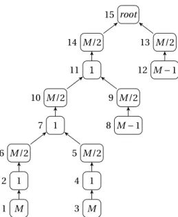
far from the optimal traversal [3]. We prove here that postorder traversals may also have bad per-formance for the MINIO problem. More specifically, we prove that there exist problem instances on which POSTORDERMINIO performs arbitrarily more I/O than the optimal I/O amount. We could ex-hibit an example where the optimal traversal does not perform any I/O and POSTORDERMINIO per-forms some I/O, but we rather present a more general example where the optimal traversal perper-forms some I/O: in the following example, the optimal traversal requires 1 I/O, when POSTORDERMINIO requiresΩ(nM) I/Os. The tree used in this instance is depicted on Figure 2(a).
It is possible to traverse the tree of Figure 2(a) with a memory of size M using only a single I/O, by executing the nodes in increasing order of the labels next to the nodes. After processing the minimal subtree including the two leftmost leaves, our strategy is to process leaves from left to right. Before processing a new leaf, we complete the previous subtree up to a node of weight 1; this way the leaf and the actives nodes can both fit in memory.
root 15 M /2 14 1 11 M /2 10 1 7 M /2 6 1 2 M 1 M /2 5 1 4 M 3 M /2 9 M − 1 8 M /2 13 M − 1 12
(a) Example of a tree showing that POSTORDERMINIO is not an approximation algorithm.
root 3 6 5 5 2 4 6 3 3 8 5 7 2 2 6 1
(b) Example of a tree where OPTMINMEMis not optimal for MINIO (M = 6). root 2k 4k + 4 3k 4k + 3 2k − 1 4k − 2 3k + 1 4k − 3
· · ·
k 4 4k 3 2k 4k + 2 3k 4k + 1 2k − 1 4k 3k + 1 4k − 1· · ·
k 2 4k 1(c) Example of a tree showing that OPTMINMEM
is not an approximation algorithm (M = 4k).
Figure 2: The label inside node i represents wi. The label next to the nodes indicate in the leftmost
On the other hand, the best postorder traversal must perform a volume of I/O equal to M /2 − 1 before it can start any leaf except for the first leaf it processes. This is because the least common ancestor of any two leaf nodes has two nodes of size M /2 as children, and all leaves have size at least
M −1. Thus, any postorder traversal incurs at least M/2−1 I/Os for all but one leaf node (3M/2−2 for
the example here). We can extend the tree in Figure 2(a): we replace root by a node of size 1, add to it a parent of size M /2 which is the left child of the new root; the right child of the new root is then a chain containing a leaf of size M − 1 and its parent of size M/2. Doing this repeatedly until n nodes are used gives the lower bound ofΩ(nM). Therefore, POSTORDERMINIO is not constant-factor competitive.
4.4
O
PTM
INM
EMis not competitive
Minimizing the amount of I/O in an out-of-core execution seems close to minimizing the peak mem-ory when the memmem-ory in unbounded. Thus, in order to derive a good solution for MINIO, it seems reasonable to use an optimal algorithm for MINMEM, such as the OPTMINMEMalgorithm presented by Liu [2], to compute a scheduleσ and then to perform I/Os using the FiF policy. In the following, we also use OPTMINMEMto denote this strategy for MINIO. We prove here that there exist problem instances on which this strategy will also perform arbitrarily more I/Os than the optimal traversal.
We first exhibit in Figure 2(b) a tree showing that OPTMINMEMdoes not always lead to minimum I/Os in our model. Let M = 6. The tree of Figure 2(b) can be completed with 3 I/Os, by doing one chain after the other. This corresponds to a peak memory of 9. But OPTMINMEMachieves a peak memory of 8 at the cost of 4 I/Os by executing the nodes in increasing order of the labels next to the nodes.
This example can be extended to show that OPTMINMEMmay perform arbitrarily more I/Os than the optimal strategy. The extended tree is illustrated on Figure 2(c). It contains two identical chains of length 2k + 2, for a given parameter k, and the memory size is set to 4k. The weights of the tasks in each chain (in order from root to leaf ) are defined by interleaving two sequences: {2k, 2k −1,...,k} and {3k, 3k + 1,...,4k}. As above, it is possible to schedule this tree with only 2k I/Os, but with a memory peak of 6k, by computing first one entire chain. However, OPTMINMEMachieves a memory peak of 5k by switching chains on each node with a weight smaller than 2k, as represented by the labels besides the nodes. Doing so, OPTMINMEMincurs k I/Os on each of the k + 1 smallest nodes, leading to a cost of k(k + 1) I/Os. The competitive ratio is then larger than k/2. Therefore, OPTMINMEMis not constant-factor competitive in the MINIO problem.
4.5 Complexity unknown
As shown above, polynomial-time approaches based on similar problems fail to even give a constant-competitive ratio. The main issue facing a polynomial approach is the highly nonlocal aspect of the optimal solution. For example, since postorder traversals are not optimal, it may be highly useful to stop at intermediate points of a subtree’s execution in order to process entirely different subtrees.
We conjecture that this problem is NP-hard due to these difficult dependencies. As mentioned above, if we require entire nodes to be written to disk, the problem has been shown to be NP-hard by reduction to Partition [3]. However, this proof depends entirely on indivisible nodes, rather than on the tree’s recursive structure. Taking advantage of the structure of our problem to give an NP-hardness result could lead to an interesting understanding of optimal solutions, and possibly further heuristics. We leave this as an open problem.
5 Heuristic
We now move to the design of a novel heuristic FULLRECEXPANDwhose goal is to improve the perfor-mance of OPTMINMEMfor the MINIO problem. The main idea of this heuristic is to run OPTMINMEM
wi
⇒
wi wi− τ(i ) wiFigure 3: Example of node expansion.
several times: when we detect that some I/O is needed on some node, we force this I/O by transform-ing the tree. This way, the followtransform-ing iterations of OPTMINMEMwill benefit from the knowledge of this I/O. We continue transforming the tree until no more I/Os are necessary.
In order to enforce I/Os, we use the technique of expanding a node (illustrated on Figure 3). Under an I/O functionτ, we define the expansion of a node i as the substitution of this node by a chain of three nodes i1, i2, i3of respective weights wi, wi− τ(i ) and wi. The expansion of a node actually
mimics the action of executing I/Os: the weight of the three tasks represent which amount of main memory is occupied by this node 1) when it is first completed (wi1= wi), 2) when part of it is moved
to disk (wi2= wi− τ(i )), and 3) when the whole data is transferred back to main memory (wi3= wi).
This technique first allows us to prove Theorem 2, which states that given an I/O functionτ, we can find a scheduleσ such that (σ,τ) is a valid traversal if there exists one.
Proof of Theorem 2. Consider the tree G0obtained from G by expanding all the nodes for whichτ is not
null. Then, consider the scheduleσ0obtained by OPTMINMEMon G0, and letσ be the corresponding
schedule on G. Then, the memory used byσ on G during the execution of a node i is the same as the one used byσ0on G0during the execution of the same node i , or of i1if i is expanded. Then, as
OPTMINMEMachieves the optimal memory peak on G0, we know thatσ uses as little main memory as possible under the I/O functionτ. Then, (σ,τ) is a valid traversal of G.
The heuristic FULLRECEXPANDis described in Algorithm 2. The main idea of the heuristic is to ex-pand nodes in order to obtain a tree that can be scheduled without I/O, which is equivalent to building an I/O function.
First, the heuristic recursively calls itself on the subtrees rooted at the children of the root, so that each subtree can be scheduled without I/O (but using expansions). Then, the algorithm computes OPTMINMEMon this new tree, and if I/Os are necessary, it determines which node should be ex-panded next. This selection is the only part where FULLRECEXPAND can deviate from an optimal strategy. Our choice is to select a node on which the FiF policy would incur I/Os; if there are several such nodes, we choose the one whose parent is scheduled the latest. After the expansion, the algo-rithm recomputes OPTMINMEMon the modified tree, and proceeds until no more I/O are necessary.
At the end of the computation, the returned schedule is obtained by running OPTMINMEMon the final tree computed by FULLRECEXPAND, and by transposing it on the original tree. The I/O perfor-mance of this schedule is then equal to the sum of the expansions.
FULLRECEXPANDis only a heuristic: it may give suboptimal results but also achieve better perfor-mance than OPTMINMEM, as illustrated on several examples Appendix A.
Unfortunately, the complexity of FULLRECEXPANDis not polynomial, as the number of iterations of the while loop at Line 3 cannot be bounded by the number of nodes, but may depend also on their weights. We therefore propose a simpler variant, named RECEXPAND, where the while loop at Line 3 is exited after 2 iterations. In this variant, the resulting tree G might need I/Os to be executed. The final schedule is computed as in FULLRECEXPAND, by running OPTMINMEMon this tree G. We later show that this variant gives results which are very similar to the original version.
Algorithm 2: FULLRECEXPAND(G, r, M ) Input: tree G, root of exploration r
Output: Return a tree Grwhich can be executed without I/O, obtained from G by expanding
several nodes 1 foreach child i of r do
2 Gi← FULLRECEXPAND(G, i , M )
3 Gr← tree formed by the root r and the subtrees Gi
4 while OPTMINMEM(Gr, r ) needs more than a memory M do
5 τ ← I/O function obtained from OPTMINMEM(Gr, r ) using the FiF policy
6 i ← node for which τ(i ) > 0 whose parent is scheduled the latest in OPTMINMEM(Gr, r )
7 modify Grby expanding node i according toτ(i) 8 return Gr
6 Numerical results
In this section, we compare the performance of the two existing strategies OPTMINMEMand POS
-TORDERMINIO, and the two proposed heuristics FULLRECEXPANDand RECEXPAND. All algorithms are compared through simulations on two datasets described below. Because of its high computa-tional complexity, FULLRECEXPANDis only tested on the first smaller dataset.
6.1 Datasets
The first dataset, named SYNTH, is composed of 330 instances of synthetic binary trees of 3000 nodes,
generated uniformly at random among all binary trees. As we considered small trees, we simply used half-Catalan numbers in order to draw a tree, similarly to the method described at the beginning of [15]. The memory weight of each task is uniformly drawn from [1; 100].
The second dataset, named TREES, is composed of 329 elimination trees of actual sparse matrices from the University of Florida Sparse Matrix Collection1(see [3] for more details on elimination trees and the data set). Our datasets corresponds to the 329 smallest of the 640 trees presented in [3], with trees ranging from 2000 to 40000 nodes.
For each tree of the two datasets, we first computed the minimal memory size necessary to process the tree nodes: LB = maxiw¯i. We also computed the minimal peak memory for an incore execution
Peakincore(using OPTMINMEM). We eliminated some trees from the TREESdataset where Peakincore=
LB, leaving us with 133 remaining trees in this dataset. In all other cases, note that the possible range
for the memory bound M such that some I/Os are necessary is [LB, Peakincore− 1]. We chose to set M
to the middle of this interval M = (LB + Peakincore− 1)/2. Simulations using other values of M in this
interval are presented in Appendix B.
6.2 Results
Our objective in this study is to minimize the total amount of I/Os needed to process the tree. In order to summarize and compare the performance of the different strategies we choose here to consider the number of I/Os and the memory bound M : performing 10 I/Os when the optimal only needs 1 does not have the same significance if the main memory consists of M = 10 slots or of M = 1000 slots. Therefore, in this section, if a schedule performs k I/Os, we define its performance as (M + k)/M.
Then, a schedule with no I/O operations has a performance of 1 while a schedule needing M I/Os has a performance of 2.
In order to compare the performance of these algorithms, we use a generic tool called performance
profile [16]. For a given dataset, we compute the performance of each algorithm on each tree and
for each memory limit. Then, instead of computing an average above all the cases, a performance profile reports a cumulative distribution function. Given a heuristic and a thresholdτ expressed in percentage, we compute the fraction of test cases in which the performance of this heuristic is at most
τ% larger than the best observed performance, and plot these results. Therefore, the higher the curve,
the better the method: for instance, for an overheadτ = 5%, the performance profile shows how often a given method lies within 5% of the smallest performance obtained.
0.00 0.25 0.50 0.75 1.00 0% 50% 100% 150% 200% 250% Maximal overhead F ract io n of test c ases 0.00 0.25 0.50 0.75 1.00 0% 10% 20% 30% Maximal overhead F ract io n of test c ases
Algorithm OPTMINMEM RECEXPAND POSTORDERMINIO FULLRECEXPAND
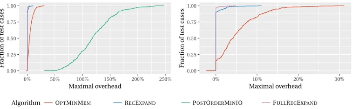
Figure 4: Performance profiles of FULLRECEXPAND, RECEXPAND, OPTMINMEM and POSTORDER -MINIO on the SYNTHdataset (right: same performance profile without POSTORDERMINIO).
The left plot of Figure 4 presents the performance profile of the four heuristics for the complete dataset SYNTH. The first result is the poor performance of POSTORDERMINIO in this dataset: it almost always has at least 50% of overhead, and even a 100% overhead in 75% of the cases. Then, RECEXPAND
performs far better than OPTMINMEM. The right plot of the figure presents the performance pro-files of exclusively OPTMINMEM, RECEXPANDand FULLRECEXPAND. RECEXPANDperforms strictly less I/Os than OPTMINMEMon 90% of the instances, and on half of them, OPTMINMEMhas a 4% overhead. We can also note that FULLRECEXPANDperforms only slightly better than RECEXPAND, but both heuristics are far ahead of OPTMINMEM, so the gain in the complexity of the algorithm is only balanced by a small loss of performance. For instance, RECEXPANDhas an overhead of more than 2% over FULLRECEXPANDon only 3% of the instances.
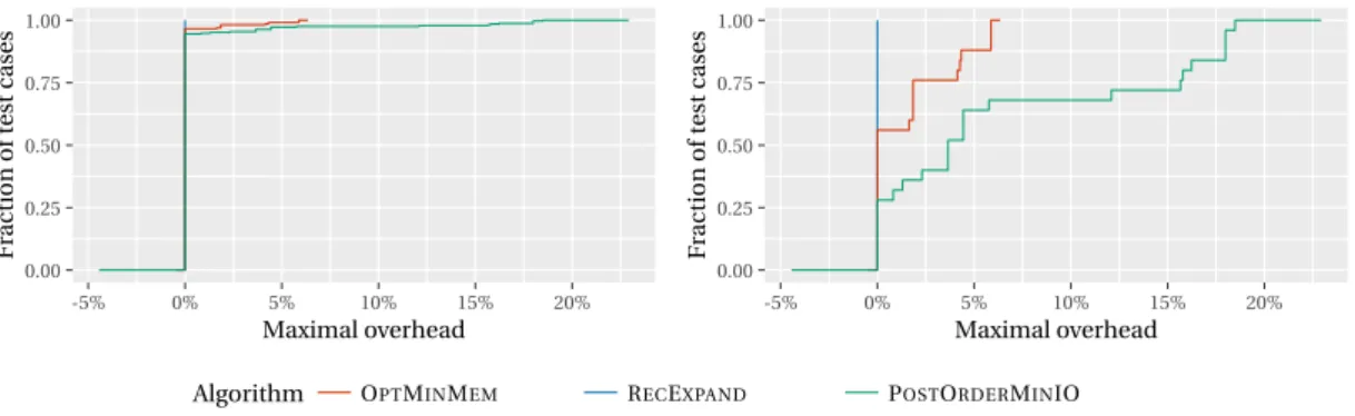
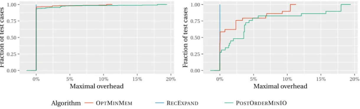
The left plot of Figure 5 presents the performance profiles of the three heuristics POSTORDER -MINIO, RECEXPANDand OPTMINMEMfor the complete dataset TREES. The first remark is that the three heuristics are equal on more than 90% of the 329 instances. Therefore, we now focus on the right plot, which presents the same performance profile for the 25 cases where the heuristics do not all give equal performance. We can see that the hierarchy is the same as in the previous dataset (RECEXPAND
is never outperformed, and OPTMINMEMperforms better than POSTORDERMINIO) but with smaller discrepancies between the heuristics. POSTORDERMINIO and OPTMINMEMrespectively have more than 5% of overhead on only 40% and 10% of these instances.
7 Conclusion
In this paper, we revisited the problem of minimizing I/O operations in the out-of-core execution of task trees. We proved that existing solutions allow to optimally solve the problem when all output data
0.00 0.25 0.50 0.75 1.00 -5% 0% 5% 10% 15% 20% Maximal overhead F ract io n of test c ases 0.00 0.25 0.50 0.75 1.00 -5% 0% 5% 10% 15% 20% Maximal overhead F ract io n of test c ases
Algorithm OPTMINMEM RECEXPAND POSTORDERMINIO
Figure 5: Performance profiles for the complete TREESdataset (left) and restricted to instances where the heuristics differ (right)
have identical size, but that none of them has a constant competitive factor compared to the optimal solution. We proposed a novel heuristic solution that improves on an existing strategy and proved very efficient in practice. Despite our efforts, the complexity of the problem remains open. Determining this complexity would definetely be a major step, although our findings already lays the bases for more advanced studies. This includes moving to parallel out-of-core execution, as we already did for parallel incore execution [4], but also designing competitive algorithm for the sequential problem.
8 Acknowledgment
This material is based upon research supported by the SOLHAR project operated by the French Na-tional Research Agency (ANR) and the Chateaubriand Fellowship of the Office for Science and Tech-nology of the Embassy of France in the United States.
References
[1] T. A. Davis, Direct Methods for Sparse Linear Systems, ser. Fundamentals of Algorithms. Philadel-phia: Society for Industrial and Applied Mathematics, 2006.
[2] J. W. H. Liu, “An application of generalized tree pebbling to sparse matrix factorization,” SIAM J.
Algebraic Discrete Methods, vol. 8, no. 3, pp. 375–395, 1987.
[3] M. Jacquelin, L. Marchal, Y. Robert, and B. Ucar, “On optimal tree traversals for sparse matrix factorization,” in Proceedings of the 25th IEEE International Parallel and Distributed Processing
Symposium (IPDPS’11). Los Alamitos, CA, USA: IEEE Computer Society, 2011, pp. 556–567.
[4] L. Eyraud-Dubois, L. Marchal, O. Sinnen, and F. Vivien, “Parallel scheduling of task trees with limited memory,” TOPC, vol. 2, no. 2, p. 13, 2015. [Online]. Available: http: //doi.acm.org/10.1145/2779052
[5] E. Agullo, “On the out-of-core factorization of large sparse matrices,” Ph.D. dissertation, École normale supérieure de Lyon, France, 2008. [Online]. Available: https://tel.archives-ouvertes.fr/ tel-00563463
[6] R. Sethi and J. Ullman, “The generation of optimal code for arithmetic expressions,” J. ACM, vol. 17, no. 4, pp. 715–728, 1970.
[7] J. W. H. Liu, “On the storage requirement in the out-of-core multifrontal method for sparse fac-torization,” ACM Transaction on Mathematical Software, 1986.
[8] P. R. Amestoy, I. S. Duff, J. Koster, and J.-Y. L’Excellent, “A fully asynchronous multifrontal solver using distributed dynamic scheduling,” SIAM Journal on Matrix Analysis and Applications, vol. 23, no. 1, pp. 15–41, 2001.
[9] P. R. Amestoy, A. Guermouche, J.-Y. L’Excellent, and S. Pralet, “Hybrid scheduling for the parallel solution of linear systems,” Parallel Computing, vol. 32, no. 2, pp. 136–156, 2006.
[10] E. Agullo, P. R. Amestoy, A. Buttari, A. Guermouche, J. L’Excellent, and F. Rouet, “Robust memory-aware mappings for parallel multifrontal factorizations,” SIAM J. Scientific Computing, vol. 38, no. 3, 2016.
[11] S. Toledo, “A survey of out-of-core algorithms in numerical linear algebra,” in External Memory
Algorithms, Proceedings of a DIMACS Workshop, New Brunswick, New Jersey, USA, May 20-22, 1998, 1998, pp. 161–180.
[12] E. Saule, H. M. Aktulga, C. Yang, E. G. Ng, and Ü. V. Çatalyürek, “An out-of-core task-based middleware for data-intensive scientific computing,” in Handbook on Data Centers, S. U. Khan and A. Y. Zomaya, Eds. Springer, 2015, pp. 647–667. [Online]. Available: http://dx.doi.org/10.1007/978-1-4939-2092-1_22
[13] L. A. Belady, “A study of replacement algorithms for a virtual-storage computer,” IBM Systems
Journal, vol. 5, no. 2, pp. 78–101, 1966.
[14] M. Lee, P. Michaud, J. S. Sim, and D. Nyang, “A simple proof of optimality for the MIN cache replacement policy,” Inf. Process. Lett., vol. 116, no. 2, pp. 168–170, 2016. [Online]. Available: http://dx.doi.org/10.1016/j.ipl.2015.09.004
[15] E. Mäkinen, “Generating random binary trees—a survey,” Information Sciences, vol. 115, no. 1-4, pp. 123–136, 1999.
[16] D. E. Dolan and J. J. Moré, “Benchmarking optimization software with performance profiles,”
A Illustration of F
ULL
R
EC
E
XPAND
on some examples
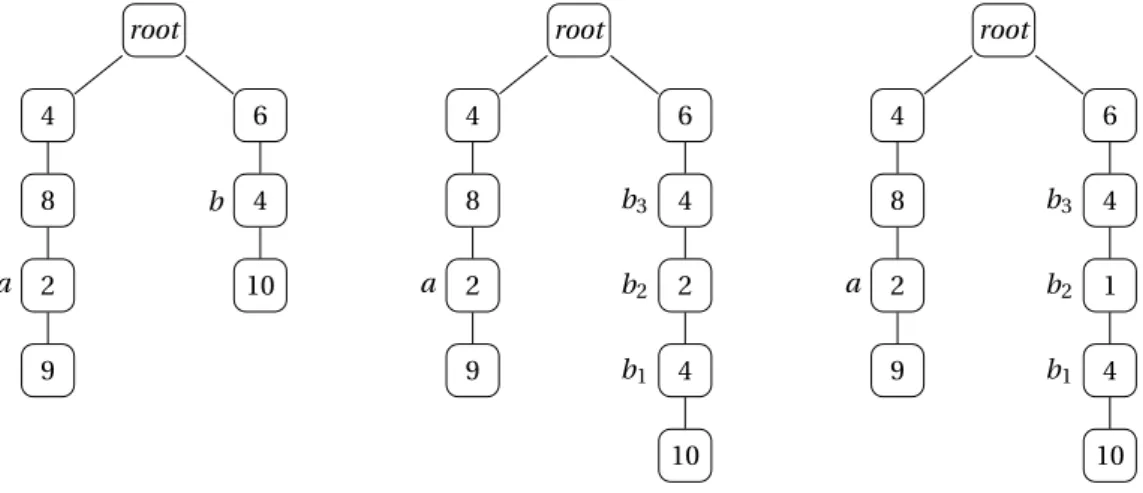
The left-hand side of Figure 6 provides an example where FULLRECEXPANDperforms better than OPT -MINMEM. OPTMINMEMcomputes the left branch first until node a, then the right branch until node
b, before completing the left branch. The memory peak reached is 12, but this schedule incurs 4 I/Os
with a memory limit of 10: 2 on node a and 2 on node b. On this example, FULLRECEXPANDexpands node b as specified on the middle diagram. With this expansion, OPTMINMEMschedules the right branch until b2first, then the whole left branch, using one more I/O on b2. This node is expanded a
second time on the right diagram, without changing the schedule obtained by OPTMINMEM, yielding to 3 I/Os on the original tree, all on b.
root 4 8 2 a 9 6 4 b 10 root 4 8 2 a 9 6 4 b3 2 b2 4 b1 10 root 4 8 2 a 9 6 4 b3 1 b2 4 b1 10
Figure 6: Example where FULLRECEXPANDis optimal whereas OPTMINMEMand POSTORDERMINIO are not. Let M = 10. The left tree is the original one, and the others are obtained during the execution of FULLRECEXPANDafter the expansion of b.
Figure 7 provides an example where FULLRECEXPANDdoes not improve OPTMINMEM. On this instance, OPTMINMEMperforms 4 I/Os, 2 on node a then 2 on node b, where POSTORDERMINIO executes first the left subtree and consumes only 3 I/Os on node c. This instance shows an example where no optimal solution perform an I/O on a node where OPTMINMEMperforms an I/O. So the
strategy of FULLRECEXPANDcannot be optimal, even if we used a different priority at Line 6.
root 3 c 2 a 7 3 4 b 7
Figure 7: Example where FULLRECEXPANDand OPTMINMEMare not optimal whereas POSTORDER -MINIO is. M = 7 in this example.
B Numerical results with other memory bounds
0.00 0.25 0.50 0.75 1.00 0% 50% 100% 150% Maximal overhead F ract io n of test c ases 0.00 0.25 0.50 0.75 1.00 0% 10% 20% 30% Maximal overhead F ract io n of test c asesAlgorithm OPTMINMEM RECEXPAND POSTORDERMINIO FULLRECEXPAND
Figure 8: Performance profile of FULLRECEXPAND, RECEXPAND, OPTMINMEM and POSTORDER -MINIO on the SYNTHdataset with the M1memory bound (right: same performance profile without
POSTORDERMINIO).
0.00 0.25 0.50 0.75 1.00 0% 5% 10% 15% 20% Maximal overhead F ract io n of test c ases 0.00 0.25 0.50 0.75 1.00 0% 5% 10% 15% 20% Maximal overhead F ract io n of test c ases
Algorithm OPTMINMEM RECEXPAND POSTORDERMINIO
Figure 9: Performance profiles for the complete TREESdataset with the M1memory bound (left) and
for the instances where the heuristics differ (right)
In this section, we present numerical results on the same datasets than the ones presented in Sec-tion 6, but with different memory bounds.
First, we use the memory bound M1= LB, which is defined in Section 6, and represents the
min-imum memory bound for which it is possible to compute a given tree. We plot the corresponding performance profiles for the SYNTHdataset in Figure 8 and the TREESdataset in Figure 9. The main conclusion that can be made comparing to the results of Section 6 is that the difference between OPT -MINMEMand RECEXPANDis significantly larger with this memory bound. Indeed, there is a 10% of overhead for OPTMINMEMin 90% of the cases whereas such an overhead was reached in only 15% of the cases previously. This can be explained by the fact that the memory bound considered here is fur-ther from the memory required by MINMEM. On the other hand, the difference between POSTORDER -MINIO and RECEXPANDare smaller in this case: there is a 100% of overhead for POSTORDERMINIO in half of the cases whereas we had this property in 75% of the cases with a higher memory bound. The same tendency can be observed for the TREESdataset in Figure 9, even if it is less significant.
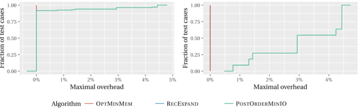
Second, we use the memory bound M2= Peakincore− 1, which is on the opposite the largest
0.00 0.25 0.50 0.75 1.00 0% 50% 100% 150% 200% Maximal overhead F ract io n of test c ases 0.00 0.25 0.50 0.75 1.00 -50% -25% 0% 25% 50% Maximal overhead F ract io n of test c ases
Algorithm OPTMINMEM RECEXPAND POSTORDERMINIO FULLRECEXPAND
Figure 10: Performance profile of FULLRECEXPAND, RECEXPAND, OPTMINMEMand POSTORDER -MINIO on the SYNTHdataset with the M2memory bound (right: same performance profile without
POSTORDERMINIO).
0.00 0.25 0.50 0.75 1.00 0% 1% 2% 3% 4% 5% Maximal overhead F ract io n of test c ases 0.00 0.25 0.50 0.75 1.00 0% 1% 2% 3% 4% Maximal overhead F ract io n of test c ases
Algorithm OPTMINMEM RECEXPAND POSTORDERMINIO
Figure 11: Performance profiles for the complete TREESdataset with the M2memory bound (left) and