Assessing Software Abstractions in WCET Analysis of Reactive Programs

HAL Id: hal-02531058

https://hal-cnrs.archives-ouvertes.fr/hal-02531058

Submitted on 3 Apr 2020

HAL is a multi-disciplinary open access

archive for the deposit and dissemination of

sci-entific research documents, whether they are

pub-lished or not. The documents may come from

teaching and research institutions in France or

abroad, or from public or private research centers.

L’archive ouverte pluridisciplinaire HAL, est

destinée au dépôt et à la diffusion de documents

scientifiques de niveau recherche, publiés ou non,

émanant des établissements d’enseignement et de

recherche français ou étrangers, des laboratoires

publics ou privés.

Assessing Software Abstractions in WCET Analysis of

Reactive Programs

Erwan Jahier, Nicolas Halbwachs, Claire Maiza, Pascal Raymond, Wei-Tsun

Sun, Hugues Cassé

To cite this version:

Erwan Jahier, Nicolas Halbwachs, Claire Maiza, Pascal Raymond, Wei-Tsun Sun, et al..

Assess-ing Software Abstractions in WCET Analysis of Reactive Programs. [Research Report] TR-2018-2,

Verimag, Université Grenoble Alpes. 2018. �hal-02531058�

Assessing Software Abstractions in

WCET Analysis of Reactive Programs

Erwan Jahier

*

_{, Nicolas Halbwachs}

*

_{, Claire Maiza}

*

_,

Pascal Raymond

*

_{, Wei-Tsun Sun}

†

_{, Hugues Cassé}

†

Verimag Research Report

n

o

TR-2018-2

February 13, 2018

*_{Univ. Grenoble Alpes/CNRS, VERIMAG F-38000 Grenoble, France}

†_{IRIT, Toulouse, France}

Reports are downloadable at the following address

http://www-verimag.imag.fr

Unité Mixte de Recherche 5104 CNRS - Grenoble INP - UGA

Université Grenoble Alpes 700, avenue centrale 38401 Saint Martin d’Hères France

tel : +33 4 57 42 22 42 fax : +33 4 57 42 22 22 http://www-verimag.imag.fr/

Assessing Software Abstractions in

WCET Analysis of Reactive Programs

3

Erwan Jahier*_{, Nicolas Halbwachs}*_{, Claire Maiza}*_{, Pascal Raymond}*_{, Wei-Tsun Sun}†_{, Hugues Cassé}†

February 13, 2018

Abstract

The estimation of the worst case execution time (WCET) of a reactive system on a given architecture is an important goal for time-critical systems. However, it cannot be achieved exactly, because of the complexity of modern architectures, the unde-cidability of most program analysis problems, and the need of taking into account the actual environment in which the system is intended to work. As a consequence, two approaches are possible: extensively testing the system with realistic input sce-narios (dynamic method) provides an under-approximation of the WCET, while a guaranteed over-approximation can be obtained by applying static analysis of soft-ware and hardsoft-ware. Comparing the results of both approaches and reducing the gap between them is interesting to assess the quality of the static analysis, and to decide when further refinements are useless. In this paper, we propose a methodology and a combination of tools to assess the result of software static analysis in the case of reactive programs. In order to permit a meaningful comparison, we perform a dy-namic analysis using a cycle accurate simulator based on the same hardware model as the one used for static analysis. Moreover, we use an existing quite sophisticated framework to conduct the generation of reactive input scenarios, in order to track the worst case. This methodology and the use of associated tools is illustrated on a small but realistic example.

Keywords: Reactive systems; Synchronous languages; Static and dynamic program analysis; Environ-ments modeling; WCET Estimation

How to cite this report: @techreport {TR-2018-2,

title = {Assessing Software Abstractions in WCET Analysis of Reactive Programs}, author = {Erwan Jahier, Nicolas Halbwachs1, Claire Maiza1, Pascal Raymond1, Wei-Tsun Sun, Hugues Cassé2},

institution = {{Verimag} Research Report}, number = {TR-2018-2},

year = {2018} }

‡_{This work has been done during the WSEPT project funded by ANR under grant ANR-12-INSE-0001.}

*_{Univ. Grenoble Alpes/CNRS, VERIMAG F-38000 Grenoble, France}

1

1

Introduction

A reactive system execution consists of a sequence of reactions, triggered either periodically or by external events. At each reaction, the system acquires inputs, updates its internal state, and produces outputs. The program that implements a reaction is usually called the transition (or step) function. Reactive systems are often referred to as safety critical, or hard real-time, meaning that missing a deadline must be considered as a functional failure. Thus, it is of great importance to know the Worst Case Execution Time (WCET) of the transition function: it allows to check whether the systems meets its timing constraints and helps to dimension its hardware requirements.

1.1

Static and dynamic WCET estimation

To get some knowledge on the WCET, one can use dynamic methods: the system is tested intensively to obtain a Measured Worst Case Execution Time (MWCET). This method is unsafe by nature: no matter how

intensive is the testing, there is no guarantee that the actual WCET has been reached. Nevertheless, this approach is widely used in industry, where the MWCET is generally corrected by some empirical factor

to obtain a reference WCET. On the other hand, static methods based on the joint analysis of the soft-ware and the hardsoft-ware, provide an Estimated Worst Case Execution Time (EWCET), which is a guaranteed

upper-bound of the actual WCET. Such safe estimations suffer from several sources of over-approximation, performed to scale-up or to cope with undecidability.

1. Hardware abstraction. The hardware behavior cannot be precisely known, because of ever-increasing complexities (caches, pipelines), and the uncertainty on the initial hardware state. The estimation uses simplified and pessimistic hardware models.

2. Software abstraction. The exact runtime behavior of the software cannot be precisely known either: the set of possible executions is overestimated as it depends on unknown data values (e.g., execution paths made impossible because of test conditions).

In this paper, we focus on assessing the imprecision of EWCET due to software abstraction.

1.2

Assessing the Overestimation

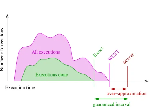
Measuring the WCET overestimation precisely is as hard as computing the actual WCET. However, MWCET

and EWCET, obtained with dynamic and static methods respectively, give a guaranteed interval for the actual

WCET, as illustrated in Figure1. The relative size of this interval can be measured by an over-estimation ratio:

ρ = (EWCET− MWCET)/MWCET

This ratio is useful for several users. The designer of a static analyzer is interested in a quantitative estima-tion of the precision of the analyzer. It is also useful for reactive systems designers to assess the realism of the evaluated WCET, or to know when it is useless to try to improve it.

1.3

Tightening the overestimation ratio

1. decrease the EWCET, with more precise static analysis;

2. increase the MWCET, with more thorough test generation.

Numerous works are dedicated to the first one. This paper focuses on the second approach, and aims at reducing the under estimation via more intensive and sophisticated testing techniques.

2 1 INTRODUCTION

Number of executions

Execution time

Mwcet

WCET

All executions

Executions done

over−approximation

guaranteed interval

Ewcet

Figure 1: Assessing the Overestimation

1.4

Assessing Software Abstractions of Reactive Programs requires fine-grained

Environment Models

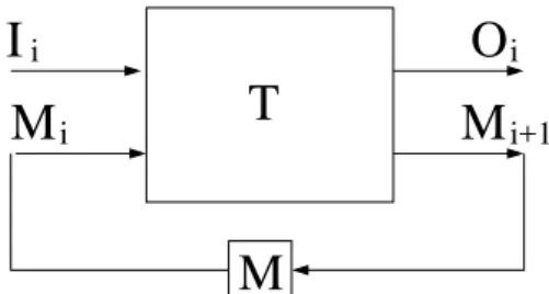
The execution of a reactive system consists of a sequence of reactions. Each reaction applies a transition function T to input values I and to a memory M (whose initial value M0is known), and returns output

values O and the new value of the internal memory; at the ithreaction, (Oi, Mi+1) = T (Ii, Mi) (cf Figure2).

Feeding T with fixed or random values for both I and M is irrelevant: the expected WCET is the one of T applied to valid input values and reachable memory states only. Providing valid inputs is complex, because reactive systems modify their environments: since reactive systems operate in closed loop with their environment, the outputs of a given reaction may influence future inputs. Moreover, the WCET may occur for some specific and rare cases: it may correspond to a memory state Mkreachable after a particular

and long input history. The probability to obtain randomly the WCET in this case can be infinitely small, and some guiding in the input generation is necessary.

Ideally, input sequences that trigger costly states should be discovered automatically by a program analysis. However, such analysis is not always possible nor tractable. Providing manually such sequences is tedious and requires a deep expertise on the system. We propose to help the system expert to generate this sequence by using Lutin [23], a programming language dedicated to the modeling and simulation of reactive systems environments. Designed for testing purposes, Lutin programs can define the set of forbidden input sequences using constraints relating inputs, outputs, and memories. Then an arbitrary number of valid input sequences can be automatically generated at random. If some more guidance is needed to put the system in some particular state, system experts can define stochastic scenarios.

1.5

The Assessment Methodology

Once the transition function is available, we compute the EWCET using static analysis tools, and the MWCET

by running random but valid (w.r.t. to inputs) simulations. If the resulting ρ is small enough, we are done. Otherwise, before trying to enhance the EWCET with more costly heuristics, we need to think about

the following question: can random inputs trigger costly parts of the transition function? If not, we can provide directly a triggering sequence of inputs. Or we can use a looser language/random-based approach, by adding more constraints, and defining stochastic scenarios.

1.6 The Experimental Setup 3

T

M

I

M

O

M

Figure 2: A transition function of a reactive program

1.6

The Experimental Setup

To compute the EWCET, we use the OTAWAframework [1], that supports the management of binary code

in general (object code loading, instructions decoding, etc.), and static WCET estimation in particular. To compute the MWCET, we use OSIM(OTAWASIMulator), a cycle-accurate simulator that we have developed

on purpose, and that is based on the OTAWAframework. The rationale for using a simulator is manifold. • Simulating rather than executing is technically much lighter and versatile.

• The actual execution platform is not always available when developing the software; and when it is, measuring faithfully the cycle numbers is complicated (probe-effect).

• It permits to assess the software abstractions more easily. Indeed, by sharing the hardware model, differences between the dynamic and the static estimation can not be due to hardware abstractions. Moreover, both tools provide profiling information on the same internal representation of the program (CFG). The user can observe that a sub-procedure is never executed, or that there is a huge difference between some loop bound estimated statically, and the number of iterations actually observed during simulations.

1.7

Contributions

This paper proposes a methodology and a tool-set to assess program analyses that compute safe WCET estimations, and to enhance the MWCET with more thorough test generation. The new part of this tool-set is

the simulation tool OSIM, connected to LUTINto simulate program environments. The paper also presents a tutorial of the LUTINlanguage which illustrates the methodology on a new representative case study. The paper also presents a new use of the LUTINlanguage: search for longest execution paths.

1.8

Paper organization

Section2describes the OTAWAWCET estimation framework, and how it has been extended to compute a MWCET. Section3presents a first set of fully automated experiments. Those experiments highlight the need

for more elaborated input generation methods. The one we propose is based on the synchronous approach; therefore the necessary background on the synchronous approach and the LUTINlanguage is surveyed in Section4. Section5illustrates the methodology on a representative case study, where LUTINis used to drive the simulation towards more precise MWCET. Section6discusses some related work.

2

Assessing WCET Estimation

WCET estimation is classically categorized into dynamic and static methods. In dynamic methods, ex-ecution time estimation is obtained from programs that are executed with a variety of input scenarios. This approach does not guarantee that the worst case is found (unless all of possible inputs and hardware configurations can be tested, which is seldom possible).

Static methods require formal models for the software and the hardware (micro-architecture). The hardware model must reflect both the functional and the temporal behaviors. Because of the complexity

4 2 ASSESSING WCET ESTIMATION Input Binary CFG Recon-struction Control-flow Graph Value Analysis Annotated CFG Basic Block Timing Info Micro-architectural Analysis Path Analysis

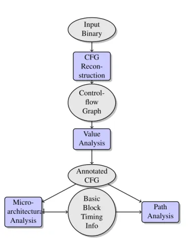
Figure 3: OTAWAframework

of the hardware and the software, models necessarily contain conservative abstractions, by considering an over-approximation of the set of actual executions.

The following sub-section briefly presents the OTAWAstatic analyzer, and how it has been extended to set up OSIM(Otawa SIMulator), a cycle-accurate simulator that uses the same hypothesis on the underlying

micro-architecture.

2.1

Background: WCET Estimation with OTAWA

OTAWA [1] is an open source framework that is able to perform execution time analysis, as sketched in Figure3. First, the binary code to analyze is transformed into a Control Flow Graph (CFG). Each CFG consists of an entry block, an exit block, and a set of Basic Blocks (BBs). Each BB contains a sequence of instructions, and BBs are connected via edges representing the control flow of the program. Each finite path between the entry and the exit block represents a potential execution.

The Value Analysis gathers and infers semantic information on the program in order to prune away execution paths that are semantically infeasible. This analysis must at least provide an upper bound for each loop in the CFG, in order to reject any infinite execution. It may be applied to the binary code, but often require the source code which is generally simpler to analyze. It may also exploit information given by the user: bounds for complex loops or recursions, or input ranges. All information are integrated as annotations into the CFG (Annotated CFG).

The Micro-architectural Analysis makes use of a model of the hardware. Its goal is to associate to each BB a temporal information, basically a local WCET. This part is highly configurable in OTAWA, via hardware models files defining the instruction set, the decoding pipeline, the memory hierarchy and cache policy. In this paper, we use a simple platform model based on a ARM7-LPC2138 architecture (3-stages pipeline), and a simple memory model without cache.

The path analysis takes the CFG with the temporal information (local WCET for each BB) and the flow information (e.g., loop bounds) and computes the worst execution path in the CFG, leading to the maximal execution time. This phase implements the Implicit Path Enumeration Technique [19], where the search of

2.2 Execution Time Measurement with OSIM 5

Figure 4: OSIMframework the worst path is expressed as an Integer Linear Program (ILP).

2.2

Execution Time Measurement with OSIM

Dynamic WCET estimation may seem quite straightforward: the program is executed on the actual archi-tecture, for a variety of input scenarios, while measuring the execution time. However, things are more complicated. First, it is not always possible to run and measure programs on the actual hardware platforms either because the hardware is not (yet) available, or because it does not provide any facility to count cycles. Moreover one has to define precisely what should be the variety of scenarios: it must contain only feasible input sequences and be large and exhaustive enough to get close to the worst case.

The tool OSIMhas been designed for this purpose, and is a contribution of this work. This section

briefly presents its main characteristics; a more detailed description can be found in a technical report [11]. OSIMis an hardware simulator based on the OTAWA framework that provides all the necessary facilities such as binary loading, decoding and instruction set simulation. The organization of OSIMis depicted in Figure4. The Structural Simulator (SS) models the control flow in the processor in a cycle accurate manner. It is developed in SystemC [8], a technology widely-used to perform cycle accurate simulations efficiently (more efficiently than VHDL-based simulations). The SS is generic and is configured via resource files to specify the characteristics of the processor and the memory (e.g., pipeline stages, memory layers, caches). This hardware description is exactly the one used by OTAWA, namely, a simple ARM7 architecture, with a 3-stages pipeline: fetch, decode, and execute. For this particular architecture, the temporal behavior is simple: the Fetch and Decode stages count for 1 cycle; the Execute stage blocks the pipeline for a variable number of cycles, depending on the type of instruction; moreover, in case of branching instructions, the pipeline flush is simulated by a penalty of few cycles (depending on the exact instruction). The instructions are virtually performed, by calling the instruction set simulator.

The instruction set simulator (ISS) is generated automatically by OTAWAfacilities. The goal of the ISS is to store and manage the functional state of the hardware: the Register file, and the Memory. Typically, a register “r1” is implemented as a field “R1” in the Register file structure. Since the temporal behavior is captured at the SS level, the simulation in the ISS is purely functional: for instance, a binary instruction like “add r1,r1,r2” is translated in a simple statement “R1 += R2;”.

2.3

Plug Lutin into O

The objective of this work is to assess the result of the static WCET estimator such as OTAWAon a par-ticular reactive program. The idea is to connect a simulator (OSIM) to an input generator that provide all necessary external input data. The objective is to be able to generate realistic and interesting scenarios for reactive programs. To be realistic, scenarios must at least satisfy some simple assumptions on input ranges, or on events exclusion. To be interesting, they also have to guide, as far as possible, the generation towards executions that are close to the worst case. Thanks to the LUTINlanguage, the user can program the generation of input scenarios. This guided test technology is presented in sections4.3and4.4. The interactions between OSIMand LUTIN, sketched-up in Figure4, are as follows:

6 2 ASSESSING WCET ESTIMATION

File MWCET EWCET ∆ ρ%

clash 56 56 0 0 expand 108 108 0 0 concat 128 128 0 0 const 56 56 0 0 extern 45 45 0 0 extern_fun 45 45 0 0 model 121 121 0 0 package 61 61 0 0 rec_nodes 324 324 0 0 unsafe_ext 38 38 0 0 fby 189 190 1 0.5 arrow 298 300 2 0.7 condact 426 428 2 0.5 red 171 173 2 1.2 dble_delay 417 420 3 0.7 merge 164 167 3 1.8 tuple 67 70 3 4.3 ck5 390 394 4 1 ck4 179 184 5 2.7 ck7 200 205 5 2.4 current 186 193 7 3.6 pusher 652 660 8 1.2 enum 228 236 8 3.4 ck6 362 371 9 2.4 expand2 280 289 9 3.1 ck3 318 328 10 3 carlights 1 465 1 477 12 0.8

File MWCET EWCET ∆ ρ%

ck2 390 403 13 3.3 matrice2 501 515 14 2.8 diese 229 243 14 6.1 fill 1 691 1 705 14 0.8 red2 569 583 14 2.5 stopwatch 1 141 1 156 15 1.3 mapinf 538 558 20 3.7 boolred 232 254 22 9.5 matrice 1 636 1 660 24 1.5 PCOND 1 463 1 502 39 2.7 minus 1 606 1 652 46 2.9 mapiter 1 528 1 576 48 3.1 modes3x2 1 164 1 221 57 4.9 with 157 231 74 47.1 struct 338 422 84 24.9 model2 3 124 3 233 109 3.5 map 889 1 099 210 23.6 is_stable 3 592 3 920 328 9.1 real 430 1 113 683 158.8 multiclock 599 1 653 1 054 176 iter 12 987 14 308 1 321 10.2 sincos 1 842 4 862 3 020 164 heater 4 102 7 224 3 122 76.1 rec_node 5 119 9 020 3 901 76.2 poly 11 482 14 927 3 445 30 speed 18 774 23 023 4 249 22.6 convertible 57 726 106 242 48 584 84.3

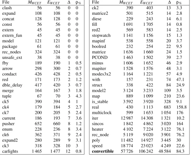
Table 1: The OTAWAand OSIMWCET estimations, in cycle numbers, on LUSTREbenchmark programs. OSIMis used with random inputs. Column 2 contains the measured Worst Execution Time (MWCET),

ob-tained among the 10 000 simulation steps. Column 3 contains the WCET upper-bound (EWCET) computed

by OTAWA. Column 4 and 5 contain the difference (∆) and the percentage ratio (ρ%) between column 3

and 2. This table is sorted out according to column 3.

• The simulator loads the binary program in the (simulated) memory (c), and the simulation starts by fetching the first instruction.

• Instructions are then handled by the classical pipeline fetch/decode/execute. During the execution, local data are read from and stored to the Register file (a) and the simulated Memory (b).

• The inputs of the simulated programs are mapped in memory at specific memory addresses. Each time the query of such an external data is recognized (i.e., at the beginning of the transition function), the input generator (e) provides a value randomly chosen among those that are compliant with the scenario.

• In the same manner, at the end of the transition function, program outputs are mapped at specific ad-dresses, which can be read by the Lutin program. This value can then be used by the input generator to produce valid or interesting values in the next step of the simulation. This point is important and specific to our framework; the test is performed in a closed loop: the program outputs may influence the validity of forthcoming program inputs.

2.4 WCET Estimation Differences 7

2.4

WCET Estimation Differences

An important characteristic of the approach is that the analysis with OTAWAand the simulation with OSIM

are based on the same model of the architecture: they have the same information on the execution time of each instruction, pipeline stages, memory load and store. Comparing results from both methods is then easier to interpret, when one wants to assess the effect of software abstractions of the WCET estimation.

When OSIMand OTAWA use the same assumptions on realistic inputs, the worst case execution time measured by OSIMis necessarily smaller or equal than the WCET estimated by OTAWA. The possible dif-ference between the two results may come from both sides (overestimation by OTAWAand underestimation by OSIM):

• Since OTAWA must guarantee an upper-bound to the WCET, any uncertainty in the abstraction must lead to a pessimistic choice.

• On the other hand, as any testing method, OSIMmay miss the actual worst input scenario.

In this work, we focus on software uncertainty rather than hardware uncertainty. We have therefore chosen a simple architecture that limits the influence of the hardware, and makes the influence of input data and execution paths more visible.

3

A Quantitative Experiment with fully automatic generation of

random inputs

This Section presents an automated experiment conducted on a set of publicly available LUSTRE pro-grams3. Then follows a discussion on the experiment interests and limitations. The goal is to show, on one hand, that for simple programs, the worst case scenario may be found without any user effort; and on the other hand, some work is necessary for more complex programs, which motivates the rest of the paper.

The experiment consists of applying the tools presented in Section2without any human intervention. A dedicated website4explains how to reproduce it. OTAWAis already an automated tool, but OSIMrequires an executable model of the environment to feed the simulated program inputs. We automate this by generating simple programs which produce random input values. Actually, this simple push-button approach can be effective at triggering costly paths in the program CFG. In Table1, the difference (∆) between the static and the dynamic approaches is often very small for this benchmark. A zero-valued ∆ means that we have actually found the actual WCET – for a given architecture abstractions, and provided that all the generated input sequences are legal. Some programs are simple, since part of this LUSTREprogram suite is made of programs written to illustrate a single LUSTREconcept at a time.

Bigger differences can be due to the pipeline analysis in presence of conditional structures (if/then/else, loops). Indeed, during the static analysis, abstract domains are used to represent the set of possible values efficiently, which lead to over-approximations at joint points. Note that loops and control structure are widely used in floating point libraries which explains the large cycle ratio (ρ) for some programs (real, sincos, speed, multiclock).

A big ρ can be helpful to hint when some unexpected software over-approximations occur. But, as ex-plained in the introduction and in Section2.4, in the case of reactive programs, it does not necessarily means that the static analyses was bad. It may also mean that costly paths can not be straightforwardly triggered during simulations. As a matter of fact, it is the case for the LUSTREprogram named convertible, which is referenced at the end of Table1. Before illustrating in Section5the use of the synchronous lan-guage LUTINto better simulate the synchronous program convertible, Section4recaps the necessary concepts of the synchronous languages.

3_{https://github.com/jahierwan/lustre-examples}

8 4 BACKGROUND: SYNCHRONOUS LANGUAGES AND TOOLS

4

Background: Synchronous Languages and Tools

A reactive system is an assembly of hardware and software that runs in closed-loop with an environment. Its execution is made of sequences of reactions. Each reaction consists of acquiring inputs, computing outputs and memories (step), and providing outputs. The synchronous approach helps designers to program the reactive step function by several means: dedicated programming languages, formal verification, and automated testing.

4.1

Languages and Code generation

Synchronous languages [2,9,17] help to design reactive systems by generating a step function, that is correct by construction with respect to the following aspects:

Bounded Memory and execution time. In order to guarantee a bound on the memory usage, synchronous languages have no dynamic data-structure; to guarantee a bound on the execution time, they have no general whileloop (for loops are possible if the number of iterations is known at compile-time). Such language restrictions also facilitate the WCET analysis.

Concurrency and determinism. Synchronous programs are made of modular unit (often called nodes) that run concurrently and communicate instantaneously without blocking (synchronous broadcast). Nodes operate over streams of values. Nodes are automatically scheduled using data dependencies. Instantaneous data dependency loops are rejected at compile-time to prevent deadlocks at runtime. Accepted programs are compiled into a deterministic single-step function made of statically-scheduled tasks – generally in C. The step function can be embedded inside an OS-free system to ensure time and functional determinism. This is essential for critical systems, to guarantee that what you simulate (or prove) during the development phase is what you execute in the final embedded device.

Clocks. By default, in data-flow programs, all expressions are executed at each step. They yield to binary code with no branch – which simplifies the WCET analysis. Yet, there is a way to prevent a computation to occur via the use of clocks. A clock is a Boolean that defines the instant when another variable is present. The clock of each variable must be declared, and the clock-consistency is checked at compile-time. For instance, consider the Lustre node speed below (used in Section5), that computes the speed (of a vehicle with wheels) out of two sampled inputs: (1) Rot, which is true each time the wheel has performed a complete rotation; and (2) Tic, which is true each time some external physical clock has emitted a signal indicating that some constant amount of time elapsed (e.g., 100 ms)5.

nodespeed(Rot, Tic:bool)returns (Speed:real); var

TicOrRot:bool; SampledSpeed:realwhenTicOrRot let

TicOrRot = TicorRot;

SampledSpeed = compute_speed(RotwhenTicOrRot, TicwhenTicOrRot); Speed =current(SampledSpeed);

tel

In this node, TicOrRot defines the instants when speed (SampledSpeed) should be updated. Hence, the only role of the speed node is to sample the input of compute_speed (using the when operator), and then to over-sample its output (using the current operator). This way, the costly compu-tations of compute_speed only occur when either Tic or Rot is true.

4.2

Formal verification

Despite guarantees provided by language restrictions and compiler analysis, synchronous programs can contain functional errors. Formal verification of temporal safety properties can be carried out via the use

4.3 Automated black-box Testing 9

of synchronous observers [10,25]. The idea is to define the program expected properties by means of a synchronous program that inputs (observes) the program inputs/outputs trace, and returns a Boolean that states whether the trace is correct or not. Trace recognizers are simpler to define than trace generators (that compute outputs out of inputs), and generally lead to orthogonal and more abstract descriptions. As most program properties are not true in any environment, hypotheses on the environment should be made. Synchronous observers defining the set of valid environment traces can be used again. The static analysis tool then explores the state-space of the synchronous product of the program, its environment, and the properties, and tries to prove that no bad state exists. Synchronous observers can formalize any safety property; and the same language can be used for the program, the properties, and the environment [21,24]. Formal verification can also be used to enhance WCET estimation, by identifying execution paths that are semantically infeasible. In synchronous programs, clocks, that state when to execute a piece of code, have a strong influence on the WCET. Detecting mutually exclusive clocks can help to lower drastically the EWCET [22].

4.3

Automated black-box Testing

The idea of the LURETTEtesting tool [15] is to re-use the observers-based formalization when the verifica-tion is too difficult because of state explosion or undecidability. The observers of expected properties can automate the test decision and play the role of the test oracle. Environment observers are used to generate the input stimuli: a Boolean-numeric solver that chooses values that satisfy the observer. Because LUSTRE

is not well-suited to express sequential scenarios, nor to assign scenario probabilities, a dedicated language, LUTIN, was designed [23,13,14].

LUTINshares with LUSTRE(most of) the syntax, the logical view of time, the structuring into concur-rent data-flow nodes, and the synchronous non-blocking broadcast semantics. The two main differences are that (1) LUTINhas some control statements to describe sequential scenarios and assign probabilities, and (2) that LUTINprograms may stop.

4.4

The LUTIN

language

We now present enough of the LUTINsyntax and semantics for the reader to understand the examples of Section5. LUTINprograms are made of two levels. The control level (or trace level) randomly chooses a constraint; and the constraint level randomly chooses values out of the chosen constraint.

More precisely, control level statements belong to a regular language over an alphabet made of con-straints. Constraints are randomly chosen (control-level non-determinism) from choices (|), sequences (fby), and Kleene stars (loop). A constraint is a relation between input, output, local, and memory variables. This relation is made of classical logic operators (not, and, or), comparisons (≤), and nu-meric expressions. Known values (inputs, memories) are propagated into the constraint, which is given to a Boolean-numeric solver6. If it is satisfiable, one solution is drawn which provides a value to outputs and locals (constraint-level non-determinism). If the elected constraint is not satisfiable, a new constraint is asked to the control-level (backtrack on choices). We now illustrate how those two levels interact using small examples. Consider the node between below, that outputs a real value x between l and h.

nodebetween(l, h:real)

returns (x:real) = (l<=xand x<=h)

If “l > h”, the constraint has no solution, and the program stops without producing any value. If “l <= h”, x is chosen uniformly in the interval [l,h] for the first step, and then the program stops. If one wants to write programs that generate more steps, one has to use a fby or a loop control-level statement. For example, the program below binds the output x to the input init at the first step, and then generates values between l and h, as long as “l < h”, for the remaining steps.

nodebetween_init(init,l,h:real)returns(x:real) = { x = init }fby

10 4 BACKGROUND: SYNCHRONOUS LANGUAGES AND TOOLS

loop{ l < x andx < h }

Hence, LUTINprograms which bodies is reduced to “loop true” generate random values forever for all their outputs. Such programs are straightforward to generate automatically and were actually used in the automated experiment presented in Section3.

The one_two node below illustrates weighted choices. A weight is an integer value attached to the branch of a choice (|int:), that indicates the relative probability of this branch to be chosen. Here, the second branch has a weight of 3, and is thus 3 times more probable than the first branch with a weight of one. Finally, this program binds x to 1 with a probability of 0.25, and to 2 with a probability of 0.75, and this behavior is repeated infinitely since no constraint can fail here.

nodeone_two()returns(x:real) = loop{ |1: x=1 |3: x=2 }

Several programs can be executed in parallel with the &> operator. For instance, in “t1 &> t2”, the LUTINinterpreter chooses a constraint c1 from t1 and c2 from t2. If “c1 and c2” is satisfiable, this conjunction is used to produce values for the step. Otherwise, the interpreter backtracks and chooses other constraints. To avoid code duplication, typed-macros can be defined via let/in statements:

letBetween(x,l,h:real):bool= (l<x) and(x<h) nodeup(init, delta:real)returns( x :real) =

{ x=init }fby

loop{ Between(x,pre x,prex+delta) }

The pre operator (as in Lustre) gives access to the previous value of a variable; pre x therefore denotes a memory. The up node binds x to init at the first step; and for the remaining steps, x is increased by a real value chosen in ]0;delta[. Another way to re-use code is by calling nodes via run/instatements. Contrary to macros, that are simply inlined, run nodes use their own runtime instance, executed synchronously. The computed output values of run nodes are injected into the context in scope, as if they were inputs or memories.

nodeup_down(min,max,delta:real)returns(x:real) = Between(x, min, max)fby

loop

existlmin, lmax, ldelta :realin runlmin := between(min,prex)in runlmax := between(pre x, max)in runldelta := between(0., delta)in {

|runx := up(prex, ldelta) inloop{ x<lmax } |runx := down(pre x, ldelta)inloop{ x>lmin } }

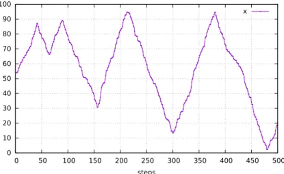
In theprogram up_down, the output x is first chosen in ]min,max[, and then the control enters an infinite loop. In this loop, local variables are chosen using the between node. The local variable values are propagated into the trace statement under scope (lines 7-10). Beside local variables definition, the loop body is made of an equiprobable choice (| – no weight means a weight of 1) : if the first branch is chosen, the node up is run, and the chosen value for x is injected into the constraint x < lmax. This constraint is used to produce up_and_down values until x < lmax becomes unsatisfiable. The control-level then backtracks and chooses the second branch of the choice, which run the down node (the dual of up) as long as x remains greater than lmin. When this second branch of the choice fails, the control is given back to the outer loop, that chooses new values for the locals, and a new branch for the choice. A 500-steps simulation of use_up_and_down is graphically represented in Figure5.

nodeuse_up_down()returns(x:real) = runx:= up_down(0.0, 100.0, 5.0)

4.5 The synchronous approach and the WCET 11 0 10 20 30 40 50 60 70 80 90 100 0 50 100 150 200 250 300 350 400 450 500 steps x

Figure 5: A 500-steps simulation ofuse_up_down

LUTIN Non-determinism is based on pseudo-randomness, which means that bugs revealed using a particular seed can be replayed7.

4.5

The synchronous approach and the WCET

The synchronous approach ensures time and functional determinism of the step function, that one tests and proves correct during the development phases. It behaves exactly the same when executed in the final embedded system. For time-triggered systems, one has to make sure that the step function execution time is smaller than the period. For event-triggered systems, the step execution time should be smaller than the reaction time of the environment. In any case, computing a tight WCET of the generated step function is necessary.

5

A detailed Experiment

We now resume the discussion of Section3, and illustrate the proposed methodology that relies on the use of the synchronous language LUTINto increase the MWCET and lower the WCET estimation ratio.

Like in Section3, this experiment is automatically run using a Gitlab CI script, and can be reproduced by anyone8_{. This section is also a tutorial demonstrating how to automate the stimulation of reactive systems.} It uses recent testing techniques, which rely on advances in language design and constraint solving (Binary Decision Diagrams and convex polyhedra). This random-based language approach is being used with some success in the industry [16].

The convertible (LUSTRE) program was designed to be realistic and to illustrate the importance of being able to take the feedback loop into account. This section starts from an empty Lutin program (that chooses all values at random) and shows how to refine it stepwisely by adding constraints and describing stochastic scenario; it also reports on the effect of such refinements on the MWCET.

5.1

The Convertible Case Study

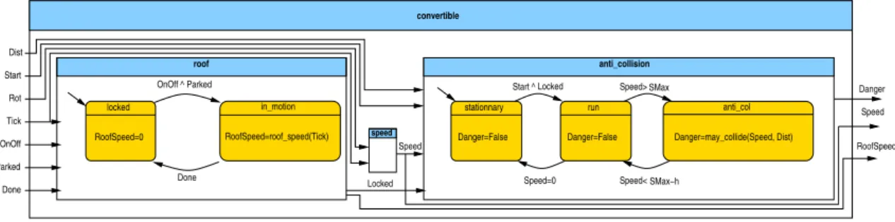
To illustrate the approach, we have designed a LUSTREprogram meant to be embedded in a car, which controls a retractable roof system and an anti-collision system. As both systems are not supposed to be active simultaneously, it makes sense to embed them into the same hardware. The retractable roof system, once activated, controls the roof motion speed, slowing it down when the roof is opened or closed at 95%.

7_{cfhttp://www-verimag.imag.fr/Lutin.htmlfor a LUTINmanual and tutorial.}

12 5 A DETAILED EXPERIMENT Danger Danger=False stationnary Speed RoofSpeed=0 Danger=False run Speed=0 Speed< roof Start Rot OnOff Parked Done speed OnOff ^ locked RoofSpeed Speed Speed> Dist anti_col Danger=may_collide(Speed, Dist) Parked Start ^ SMax−h SMax Locked Locked Done Tick in_motion RoofSpeed=roof_speed(Tick) anti_collision convertible

Figure 6: Theconvertibleprogram. The Locked variable is true when the roof is in the locked state. Speedis computed out of Tick and Rot by the speed node presented in Section 4.1. SMax is the speed that triggers the anti-collision mode. h is a small constant used to avoid hysteresis between the run and the anti_col states. roof_speed(Tick) and may_collide(Speed,Dist) are auxiliary (costly) nodes not detailed here.

The anti-collision system, activated when the vehicle goes beyond a certain speed, uses the distance from the vehicle at the front to emit an alarm. The system inputs are:

• Rot, which is true when the wheel has performed a rotation. Tick, which is true when a constant period of time has elapsed. Rot and Tick are used to compute the vehicle Speed (cf Section4.1). Tickis also used to compute the percentage of roof opening.

• Parked is true when the vehicle is parked. OnOff is true when the driver asks to open or close the roof. Done is true when the roof finishes to close or open.

• Start is true when the driver wants to start the vehicle. Dist is the distance to the vehicle at the front. Startand OnOff comes from driver requests; the other inputs come from sensors. From inputs, the program computes two outputs:

• Danger signals that the vehicle is too close to the front one (computed from Speed and Dist). • RoofSpeed is a real that controls the speed of the roof.

This program is represented in Figure6using block-diagrams (sharp corners) and automata (rounded corners). The complete LUSTREprogram (250 loc) is part of public git repository3. Each sub-system has different modes of computations, and each mode has different computation times. They are running in parallel, but the costly modes are exclusive. The costly modes of the roof system goes on when the roof is opening/closing to compute the roof speed by counting Tick; and the costly mode of the anti-collision system is active when the vehicle exceeds some speed. Since the system ought to make sure that the roof is not in motion when the vehicle runs, those two costly modes ought to be exclusive. To be efficient, the automaton encoding heavily relies on LUSTREclocksthat allow to state when a computation should occur. The LUSTREV6 compiler generates from this program a 1500 loc C step function, which is compiled using a gcc ARM cross-compiler. OTAWAanalyzes the resulting binary using an ARM7 configuration (LPC2138) and computes a worst case of 106 242 cycles. To compute this number of cycles, OTAWA

assumes that all inputs and all configurations of the program memories are possible.

5.2

Tightening the overestimation ratio

In order to assess the EWCET, engineers can perform simulations with OSIM, which measure the cycle

counts at each step, and look how far the longest simulation step is from the EWCET. It is a difficult and

tedious job to provide all the inputs for the simulation of reactive programs. LUTIN, which was designed to model reactive programs environments for testing purposes, can be used in this context.

5.2 Tightening the overestimation ratio 13 0 500 1000 1500 2000 0 30000 60000 90000

Number of Cycles

Cycles counts

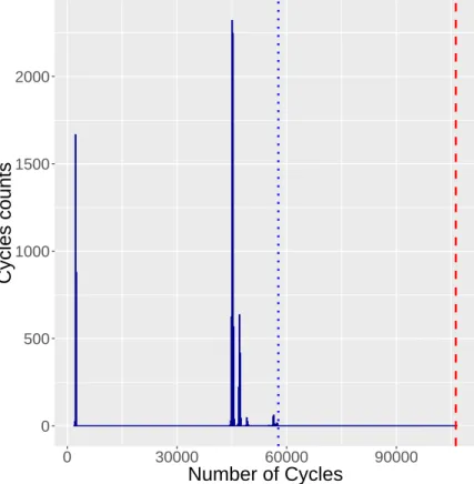
Figure 7: Cycle counts distribution obtained with env1 and OSIMon a 10 000 steps simulation. The dotted line (left, in blue) materializes the longest simulation. The dashed line (rigth, in red) represents the WCET computed by OTAWA.

5.2.1 A fully random Environment

The simplest LUTINenvironment is the one that has no constraint (true) for all instants (loop):

nodeenv1()returns(

Dist:real; Start,Parked,Rot,Tick,OnOff,Done:bool) = looptrue

Hence, at each step, all output variables are chosen equi-probably at random – as we did in Section3

to provide inputs to benchmark programs.

We run this env1 environment with the convertible step (transition) function via OSIM for 10 000 steps – which lasts a several minutes on a recent PC. Figure7shows the distribution of cycle counts for each step function call. We can see that most of the steps last for either around 800 cycles, or around 45 000 cycles. A smaller group of steps lasts longer (around 57 000 cycles), and contains the longest one that lasts 57 726 cycles.

5.2.2 Forbidding impossible inputs

Several hypotheses on the program inputs can be taken into account to refine the WCET estimations. H1: The driver can start the vehicle and action the roof at the same time.

H2: As long as the the vehicle is parked, the wheel rotation sensor do not emit any event. H3: As long as the the vehicle speed is not null, the car is not parked.

14 5 A DETAILED EXPERIMENT

By applying the method described in [22], the LESAR[24] model-checker can use those hypotheses to discover infeasibility paths in the binary Control Flow Graph. More precisely, LESARautomatically finds that states in_motion and anti_col (of Figure6) are never active at the same time, as a consequence of hypothesis H1. This information is translated into exclusion properties at the binary level, and taken into account by OTAWAthat gives an improved EWCET of 64 042 cycles (i.e., an improvement of 60%).

As far as the MWCET is concerned, one can formalize those four assumptions using theenv2LUTIN program:

nodeenv2(Speed,Roof_Speed:real)returns(

Start,Parked,Rot,Tick,OnOff,Done:bool; Dist:real) = {

loop{not(OnOffandStart) }-- H1 &>loop{ Parked =>notRot }-- H2 &> truefby loop{

( Speed > 0.0 =>notParked )-- H3 and ( Roof_Speed > 0.0 =>notDone )-- H4 }

}

All hypotheses are executed in parallel branches – using the &> operator. The third and fourth assump-tions begin with the true statement, which means that no constraint is used in the corresponding branches during the first instant. This is necessary because they involve inputs, which are not available at the very first step. Notice here the importance of the feedback loop again: it allows the environment to react to the value of the vehicle speed, which is a program output. Such kind of input sequences can not be generated offline.

During a 10 000 steps long simulation, the longest step of the convertible program using the env2 environment was made of 45 612 cycles (cf Figure8). However, such simple environments (env1 and env2) can not always trigger all the program corner cases. In this example, since the probability of having a Rot is the same as having a Tick (and depending on the wheel girth and the step activation period), the test engineer may never trigger the anti_col state. The vehicle would not move fast enough to switch the anti-collision system on.

5.2.3 Defining scenarios to visit more paths

To obtain a better simulation-based estimation, we need to write scenarios that put the program into inter-esting states. Here, the test engineer could design a deterministic program that performs enough rotations per second to make the vehicle move fast enough to enter the anti_col state. However, that would not be in the spirit of the language, where everything is random by default. It is better when designing envi-ronment models to remain as loose as possible, giving a chance to the randomness to trigger corner cases – which means, in a WCET perspective, to visit new paths in the control-flow graph.

letgeneRotTick(Start,Rot,Tick,Danger:bool): trace = letdecel = { |5:notRot |1: Rot } in

letaccel = {{ |1:notRot |5: Rot } &> Start &> notDanger} in

loop[50]notRotfby loop{

loop[0,300] accelfby loop[0,300] decelfby loop[60,300]notRot }

In geneRotTick, we first generate 50 steps where the only constraint is that Rot is false (line 6) to model the fact that a vehicle is first parked for a while; then we enter an infinite loop (line 7), made of an acceleration stage (line 8), followed by a deceleration stage (line 9), each stage lasting between 0 and 300

5.2 Tightening the overestimation ratio 15 0 1000 2000 3000 0 20000 40000 60000

Number of Cycles

Cycles counts

Figure 8: Cycle counts distribution obtained with env2 and OSIMon a 10 000 steps simulation. The dashed (rigth-most) line represents the WCET computed by OTAWA, with the path analysis described in [22].

16 5 A DETAILED EXPERIMENT

Method used OSIMwithout OSIMwith OTAWA

scenario (env1) scenarios (env3)

WCET 57 726 71 352 106 242

Table 2: The WCET estimations obtained without any hypothesis on the environment

steps. The deceleration stage is defined with the decel macro (line 2), which states that a Rot is 5 times less likely to happen than not to happen, whereas in the accel macro (line 3), a Rot is 5 times more likely to happen. The macro accel additionally enforces Start to be true (the “&>” operator conjuncts trace expressions), to reflect the fact that a vehicle only moves when someone ask to start it on. The constraint not Dangerhas a different nature, since Danger is an input; when Danger is true, the whole accel constraint is false, and the acceleration loop is forced to exit.

Note the feedback loop here: when Danger is true, the accel mode is inhibited to model the fact that the driver ought to stop accelerating when a danger arises; such behavior cannot be simulated offline. Even if it seems less realistic, it might be interesting from the coverage point of view to remain longer in this mode to explore more paths. A refinement could be to accept such behavior, but with a lower probability.

nodeenv3(Danger:bool)returns (

Start,Parked,Rot,Tick,OnOff,Done:bool; Dist:real) = runDist := up_down(0.0, 500.0, 5.0)in

not(StartorRotorTick)

fbygeneRotTick(Start, Rot, Tick, Danger)

The geneRotTick macro can then be used to define athird vehicle environment env3. Here, for didactic purposes, we do not forbid impossible inputs as we do in Section5.2.2. At the first instant, we carefully avoid to use the geneRotTick macro, because it uses the Danger input, which is not avail-able yet. In parallel of the generation of the outputs Start, Rot, and Tick, the node up_and_down presented in Section4.4generates the distance (Dist) to the front vehicle. Figure9shows the distribution of cycle counts obtained on 10 000 steps using this environment, which maximum is 71 352 cycles. This simulation does not take into account any property on the environment, and in particular the exclusivity of Startand OnOff. The results of this experiment is outlined and compared with the first one in Table2. 5.2.4 Combining all environments

Theenv4LUTINprogramcombines the constraints of env2 and env3, and produces a 60 371 cycles

simulated WCET (Figure10).

nodeenv4(Danger:bool;Speed,Roof_Speed:real)returns (Start,Parked,Rot,Tick,OnOff,Done:bool; Dist:real) =

runDist := up_down(0.0, 500.0, 5.0)in {

not(StartorRotorTick)

fbygeneRotTick(Start, Rot, Tick, Danger) &>loop{not(OnOffandStart) }-- H1 &>loop{ Parked =>notRot }-- H2 &> truefby loop{

( Speed > 0.0 =>notParked )-- H3 and( Roof_Speed > 0.0 =>notDone )-- H4 }

}

The results of the simulations performed by OSIMusing LUTIN environments env2 and env4 on the convertible program are summarized in Table3. Note that the WCET obtained by simulation of an environment that generates impossible inputs (where both OnOff and Start are true at the same instants) overtakes the WCET computed by OTAWAand LESARthat takes into account the hypotheses on inputs.

5.2 Tightening the overestimation ratio 17 0 1000 2000 0 30000 60000 90000

Number of Cycles

Cycles counts

Figure 9: Cycle counts distribution obtained with env3 during a 10 000 steps simulation. The rigth-most dashed line represents the WCET (in red) computed by OTAWA without taking into account any environment property.

Method OSIMwithout OSIMwith OTAWA

used scenario (env2) scenarios (env4) + LESAR

WCET 45 612 60 371 64 042

18 5 A DETAILED EXPERIMENT 0 1000 2000 0 20000 40000 60000

Number of Cycles

Cycles counts

Figure 10: Cycle counts distribution obtained with env4 and OSIMon a 10 000 steps simulation. The rigth-most dashed line represents the WCET computed by OTAWA, with the path analysis described in [22].

19

This is precisely because those 2 numbers are not comparable that we present the results in 2 different tables (Tables2and3).

6

Related work

This work is related to the abundant literature on test input generation for reactive systems [3,27]. Works targetting WCET estimation uses random test generation and model-checking [26], genetic algorithm [20], path clustering [5] or profiling [12]. All those works use (source or binary) code analysis to perform input generation, while we focus on environment modeling and whether inputs are feasible and relevant, which is complementary.

Performing dynamic WCET measurements with the help of a model of the environment is not common. To our knowledge, the most similar approach is presented in [7]. The main difference with our work is that the environment is described (and simulated) with Matlab-Simulink. Simulink is well suited for modeling continuous time, deterministic, and physical environment. LUTINwhich was designed for testing purpose, is more suitable and versatile for describing and simulating stochastic scenarios: with a compact description and a intensive automatic testing, the LUTINframework can exercize automatically a lot of corner-case configurations.

A main goal of this work is to assess the quality of the static WCET analyses, by performing simulations using the same micro-architecture model. A similar idea exists in the Chronos tool [18], but the inputs are provided manually. We argue here that for reactive systems (sometimes also named dynamic systems), providing a static set of input traces is not sufficient, because of the program outputs may modify the environment (feedback loop). It is therefore necessary to execute the program in a simulated reactive environment.

Other methods aim at quantifying the precision of estimations based on the uncertainty of the hardware analysis [4]. Usual hardware analyses (like caches) use categorization approach: some categories are precise (always hit or miss) while others are not (not classified). The latter categories are often sources of overestimation as the WCET analysis consider their worst time: the idea is then to compare WCETs accounting the worst and the best time of these categories to qualify the precision.

7

Conclusion

We have presented a tool-based methodology to assess the quality of sofware abstractions used in the con-text of static WCET estimation of reactive programs. We have developed OSIM to simulate an ARM7 platform using the same hardware description as in the static WCET tool OTAWA. Furthermore, we have connected OSIMto an environment model using the existing LUTINlanguage. We have shown on a rep-resentative reactive program that the environment model plays an important role in the measured WCET estimation.

The tool-chain allows users to assess the work of the static analyzer for a given hardware model and a given program. Note also that this approach can hint when there is a large over-approximation, but some investigation is still needed to understand where it comes from. For this purpose, OSIMis able to decorate the executable Control Flow Graph with the number of times each basic block and edge was taken.

Since OTAWAanalyzes binary code, and LUTINinteracts with black-box programs, the tool chain can be used with any kind of reactive programs. They may come from Scade or Simulink code generators for example, or even be directly written in C.

The whole approach could be adapted to industrial static analysers such as ABSINT[6], provided that they have a simulator. From the environment modeling point of view, test engineers could use the STIMU

-LUSworkbench [16] that offers capabilities similar to LUTIN.

Acknowledgments

Mamadou Ouologuem helped with the design of the LUSTREexample during a one-month first-year in-ternship.

20 REFERENCES

References

[1] C. Ballabriga, H. Cassé, C. Rochange, and P. Sainrat. OTAWA: an Open Toolbox for Adaptive WCET Analysis (regular paper). In IFIP Workshop on Software Technologies for Future Embedded and Ubiquitous Systems (SEUS), octobre 2010.1.6,2.1

[2] G. Berry and G. Gonthier. The Esterel synchronous programming language: Design, semantics, implementation. Science of Computer Programming, 19(2), 1992. 4.1

[3] M. Broy, B. Jonsson, J.-P. Katoen, M. Leucker, and A. Pretschner. Model-Based Testing of Reactive Systems: Advanced Lectures (Lecture Notes in Computer Science). Springer-Verlag New York, Inc., Secaucus, NJ, USA, 2005. 6

[4] H. Cassé, H. Ozaktas, and C. Rochange. A Framework to Quantify the Overestimations of Static WCET Analysis. In 15th Int. Workshop on Worst-Case Execution Time Analysis (WCET 2015), volume 47, 2015. 6

[5] J-F. Deverge and I. Puaut. Safe measurement-based WCET estimation. In Int. Workshop on Worst-Case Execution Time (WCET) Analysis, 2005. 6

[6] C. Ferdinand and R. Heckmann. ait: Worst-case execution time prediction by static program analysis. In Building the Information Society. 2004. 7

[7] J. Garrido, D. Brosnan, J. Antonio de la Puente, A. Alonso, and J. Zamorano. Analysis of WCET in an experimental satellite software development. In 12th Int. Workshop on Worst-Case Execution Time, 2012. 6

[8] Frank Ghenassia et al. Transaction-level modeling with SystemC. Springer, 2005. 2.2

[9] N. Halbwachs, P. Caspi, P. Raymond, and D. Pilaud. The synchronous dataflow programming lan-guage Lustre. Proceedings of the IEEE, 1991. 4.1

[10] N. Halbwachs, F. Lagnier, and P. Raymond. Synchronous observers and the verification of reactive systems. In Algebraic Methodology and Software Technology. 1994. 4.2

[11] Wei-Tsun Sun. A framework for simulate synchronous reactive programs and measure execution times to aid wcet analysis. Technical Report 27-06-2016, Verimag Research Report, 2016.2.2

[12] E. Y-S. Hu, A. J. Wellings, and G. Bernat. Deriving java virtual machine timing models for portable worst-case execution time analysis. In OTM Workshops, 2003. 6

[13] E. Jahier, S. Djoko-Djoko, C. Maiza, and E. Lafont. Environment-model based testing of control systems: Case studies. In TACAS, 2014.4.3

[14] E. Jahier, N. Halbwachs, and P. Raymond. Engineering functional requirements of reactive systems using synchronous languages. In Int. Symp. on Industrial Embedded Systems, 2013. 4.3

[15] E. Jahier, Pascal R., and P. Baufreton. Case studies with lurette v2. Software Tools for Technology Transfer, 8(6), 2006. 4.3

[16] Bertrand Jeannet and Fabien Gaucher. Debugging embedded systems requirements with Stimulus: an automotive case-study. In 8th European Congress on Embedded Real Time Software and Systems (ERTS 2016), 2016.5,7

[17] P. LeGuernic, A. Benveniste, P. Bournai, and T. Gautier. Signal, a data flow oriented language for signal processing. IEEE-ASSP, 1986. 4.1

[18] X. Li, L. Yun, T. Mitra, and A. Roychoudhury. Chronos: A timing analyzer for embedded software. Sci. Comput. Program., 2007.6

REFERENCES 21

[19] Y.-T. S. Li and S. Malik. Performance analysis of embedded software using implicit path enumeration. In Workshop on Languages, Compilers, and Tools for Real-Time Systems, pages 88–98, 1995. 2.1

[20] P. Puschner and R. Nossal. Testing the results of static worst-case execution-time analysis. In Pro-ceedings of the 19th IEEE Real-Time Systems Symposium, Madrid, Spain, December 2-4, 1998, 1998.

6

[21] C. Ratel, N. Halbwachs, and P. Raymond. Programming and verifying critical systems by means of the synchronous data-flow programming language lustre. In ACM-SIGSOFT’91 Conference on Software for Critical Systems,New Orleans, December 1991. 4.2

[22] P. Raymond, C. Maiza, C. Parent-Vigouroux, and F. Carrier. Timing analysis enhancement for syn-chronous program. In Proceedings of the 21st Int. Conference on Real-Time Networks and Systems, 2013.4.2,5.2.2,8,10

[23] P. Raymond, Y. Roux, and E. Jahier. Lutin: A language for specifying and executing reactive scenar-ios. EURASIP Journal on Embedded Systems, 2008, 2008. 1.4,4.3

[24] Pascal Raymond. Synchronous program verification with lustre/lesar. In Modeling and Verification of Real-Time Systems, chapter 6. ISTE/Wiley, 2008.4.2,5.2.2

[25] John Rushby. The versatile synchronous observer. In Specification, Algebra, and Software. 2014.4.2

[26] I. Wenzel, R. Kirner, B. Rieder, and P. Puschner. Measurement-based timing analysis. In Int. Sympo-sium on Leveraging Applications of Formal Methods, Verification and Validation, 2008. 6

[27] J. Zander, I. Schieferdecker, and P. J. Mosterman. A Taxonomy of Model-based Testing for Embedded Systems from Multiple Industry Domains, chapter 1, pages 3–22. CRC Press, 2011.6