Cell fleet planning : an industry case study

FTL COPY, DONT R EMOVE

FTL Report R84-4

Cell Fleet Planning: An Industry Case Study

Armando C. Silva

FTL Report R84-4

Cell Fleet Planning: An Industry Case Study

Armando C. Silva

CELL FLEET PLANNING: AN INDUSTRY CASE STUDY by

ARMANDO C. SILVA

Submitted to the Department of Aeronautics and Astronautics on May 11, 1984 in partial fulfillment for the requirements

of the Degree of Master of Science in Aeronautics and

Astronautics

ABSTRACT

The objective of this thesis is to demonstrate the

practical use of the Cell Fleet Planning Model in planning the fleet for the U.S. airline industry. The Cell Model is a

cell-theory, linear programming approach to fleet planning.

Four scenarios of the Model are presented: three with a

nine-cell representation of the system and a test case using a thirty-cell representation. A detailed analysis of the results

for each case has been performed. A comparison between the cases,

with other forecasts, and with recent historical data which has

also been .analyzed is shown.

The Cell Model has produced realistic results. It has

proven to be efficient regarding computer time and labor intensity given the size of the problem, and to be viable for industry use. Should no dramatic changes in the airline route system structure occur in the next ten years, results obtained show a greater need for small-capacity, short-range aircraft

(e.g. B737's, B757's, and DC9's) than for other aircraft types.

Thesis Supervisor: Robert W. Simpson

Title: Professor of Aeronautics and Astronautics

Thesis Supervisor: Dennis F.I. Mathaisel

ACKNOWLEDGEMENTS

I wish to express my deepest gratitude to Dr. Dennis F.X. Mathaisel, whose guidance and advise made possible this thesis. My thanks

to Prof. Robert W. Simpson, Director of the Flight Transportation Laboratory and supervisor of this thesis. I also wish to thank N.George Avram, William P. Dickens, and Lawrence G. Moran of the Pratt & Whitney Aircraft Group and Lee H. Dymond of Synergy, Inc. Washington D.C. for their valuable help. My gratitude to my wife, Malena, for her love, patience, help, and support through the completion of this work. Thanks

to all my friends at the Flight Transportation Laboratory, teachers, staff, and fellow students, for their encouragement through the

TABLE OF CONTENTS

CELL FLEET PLANNING: AN INDUSTRY CASE STUDY

Chapter 1. Introduction ... . ...

--Chapter 2. Cell Fleet Planning ...-.

.--2.1 Cells: Definition and Clustering 2.1.1 Grid Cells and Cluster Cells

2.1.2 Number of Cells

2.1.3 Cell Attributes ...

2.1.4 Elements of a Cell ...

2.1.5 Cell Forecasting - Cell Matching

2.2 Demand-Frequency Curves

2.3 Mathematical Structure of the Cell Fleet

Planning Model ... 2.3.1 Objective Function 2.3.2 Constraints ... ... 2.3.2.1 Demand Carried ... 2.3.2.2 Sum of Frequencies ... 2.3.2.3 Load Factor 2.3.2.4 Frequency Range ... 2.3.2.5 Fleet Utilization 2.3.2.6 Fleet Continuity

Chapter 3. Industry's Fleet Composition in Recent Years

10 16 17 17 19 20 22 24 25 30 30 31 31 32 32 33 33 34 Ak

Chapter 4. Application of the Cell Fleet Planning Model: A Case Study ...

4.1 Computer Implementation of the Cell Fleet Planning Model ...

4.2 Inputs

4.2.1 Aircraft Selection Table ...

4.2.2 Parameters Table ...

4.2.3 Aircraft Input Table 4.2.4 System Costs Table 4.2.5 Cell Data Table ...

4.2.6 Demand-Frequency Data

4.2.7 Aircraft Load Factors Table ...

4.2.8 Aircraft Fuel Consumption Table 4.2.9 Minimum and Maximum Fleet Count

by Year Table ... 4.2.10 Utilization Table ... 4.3 Outputs ... 4.3.1 4.3.2 4.3.3 4.3.4 4.3.5 4.3.6 4.3.7 Table Table Table Table 1-1: Aircraft Inventory . 1-2: Aircraft Acquisition 1-3: Aircraft Retirement 2: Percent Departures by by Type aell 000* 54 54 55 55 56 56 57 58 61 61 62 63 63 64 64 64 64 65 65

Table 3: Operating Statistics ...

Table 4: Financial Statistics Report Table 5: Aircraft Activity for Each

Chapter 5. Analysis of Results ... .

5.1 Analysis of Results for the Nine-Cell Cases ....

5.1.1 Nine Cells, Case A ...

5.1.2 Nine Cells, Case B ...*... *** 5.1.3 Nine Cells, Case C ... .. 5.2 Analysis of the Thirty-Cell Case and

Comparison to the Nine-Cell Case

5.3 Comparison of the Cell Fleet Planning Model

Results to Historical Data ...

5.4 Comparison to Other Forecasts ....

5.4.1 F.A.A. Forecasts ...

5.4.2 McDonnell Douglas Forecasts

5.4.3 Boeing Forecasts ...

5.4.4 Pratt & Whitney Forecasts* ...

Chapter 6. Appendix A.1 Appendix Appendix Appendix Appendix A.2 A.1 B.1 B.2 Conclusions ...

Historical Daily Frequency for Selected Aircraft Types per Cell ...

:Aircraft Codes o...

: Historical Weekly Frequency for All Aircraft

Types per Cell ...

: Input Tablestailed.C... :Sample of Detailed Cell Results ...

Appendix C: Computer Statistics ...

96 96 109 121 132 137 142 142 146 147 148 151 154 200 201 247 274 277 279 References .. . .. .. . . . ..

List of Figures

Figure Page

1.1 Boeing's Airplane Forecast Methodology Flow Diagram 14

2.1a Example of Grid Cells 18

2.1b Example of Cluster Cells ... 18

2.2 Within-Cluster Sum of Squares vs. Number of Cells Plot . 21 2.3 Sample of OAG Database 23 2.4 Demand-Price Curve ... 27

2.5 Demand-Time Curve ... 27

2.6a Demand-Frequency Curve ... 29

2.6b Approximated Demand-Frequency Curve ... 29

3.1 Average Number of Aircraft Assigned to Service per Aircraft Group (1979-82) ... 42

4.1 Flowchart of the Cell Fleet Planning Model ... 53

4.2a Demand-Frequency Curve for Cell No. 1 (Nine-Cell Case) .. 59

4.2b Demand-Frequency Curve for Cell No. 4 (Nine-Cell Case) .. 60

5.1 Number of Aircraft per Generic Group (Case A) ... 99

5.2 Number of Aircraft per Generic Group (Case B) ... 112

List of Tables

Table Page

3.1 Composition of Aircraft Groups ... 37

3.2 Average Number of Aircraft Assigned to Service per Individual Type ... 38

3.3 Average Number of Aircraft Assigned to Service per Aircraft Group ... 40

3.4 Historical Daily Frequencies per Aircraft Type ... 43

3.5 Examples of Segments in Each Cell for 1983 ... 45

3.6 Daily Frequencies per Aircraft Group ... 48

5.1 Number of Aircraft per Generic Group for Case A ... 98

5.2 Daily Frequencies per Aircraft Type per Cell (Case A) .. 102

5.3 Total Daily Frequencies per Generic Group for Case A ... 108

5.4 Number of Aircraft per Generic Group for Case B ... 111

5.5 Daily Frequencies per Aircraft Type per Cell (Case B) .. 114

5.6 Total Daily Frequencies per Generic Group for Case B ... 120

5.7 Number of Aircraft per Generic Group for Case C ... 122

5.8 Daily Frequencies per Aircraft Type per.Cell (Case C) .. 125

5.9 Total Daily Frequencies per Generic Group for Case C ... 131

5.10 Number of Aircraft per Generic Group for the Thirty-Cell Case ... 133

5.11 Total Daily Frequencies per Generic Group for the Thirty-Cel1 Case ... 135

5.12 C.A.B. and Cell Model Operating Statistics for 1982 .... 138

5.13 Comparison of Historical and Cell Model Daily Frequencies ... 140

Table Page 5.14a Revenue Passenger Miles (RPM) Forecasts ... 143 5.14b Available Seat Miles (ASM) Forecasts ... 144 5.15 F.A.A. Forecasts on the Number of Aircraft per

Generic Group ... 145

CHAPTER 1.

INTRODUCTION

Aircraft fleet planning is, in simple terms, the process of

answering the following five questions:

- How many aircraft will be needed

- What types of aircraft will be needed

- When are these aircraft to be acquired - Where are these aircraft to be allocated - How will these aircraft be financed

The aircraft selection process is influenced by a wide range of

factors including economic, technological, financial, regulatory/ political, environmental, foreign manufacturer competition, and marketing

factors. Among the economic factors, the selection process has to

consider aircraft productivity defined in terms of available seat miles

(ASM) per aircraft. An ASM is defined as:

ASM = Capacity * Speed * Utilization

Traffic forecasts are extremely important in the fleet planning process. They constrain the market and finally determine the number of seats that

will be required in the future. Traffic forecasts define the demand for which the fleet planning process searches the corresponding supply. Operating expenses is another very important economic factor. The goal

of fleet planning is to determine the aircraft type at the proper moment in time that will maximize revenues and minimize operating expenses. The

objective of an airline, agency, government, or whoever performs the fleet planning, may not be to maximize profits but, for example, to

a state-owned airline and that views air transport exlusively as a public

service. But even then, the idea is to maximize service at the least

possible cost.

The route structure is of great significance in the aircraft selection. The payload-range characteristics of the aircraft must match the requirements of the route structure. A route structure conformed by a majority of short-haul low-demand segments will require a greater number of short-range small-capacity aircraft, since these are the most

efficient aircraft types for routes with those characteristics, and

viceversa.

The technological factors of aircraft selection involve

operations-related and maintenance-operations-related factors. Among the operations-related

factors are the flight performance characteristics, the ground operations

requirements, airport constraints, air compatibility, and cargo convertibility. Maintenance-related factors can include: service records, parts pools, fleet commonality and product support.

Regulatory and/or political factors also influence the aircraft

selection process. Airline deregulation, needless to say, has had a great

impact on U.S. airline industry and has been the cause for major changes

in route structures. Many studies on the effect of deregulation have been

and continue to be made. As a political factor, one could list the foreign governments' support of exports, which translate into export credit financing, tax incentives, direct promotion and assistance. Noise

compliance regulations are an example of regulatory and environmental factors affecting aircraft selection.

The aircraft fleet planning process varies according to the sector performing this planning. A different approach is carried, for example,

by an airline than by an engine or airframe manufacturer. A fleet

planning process by an airline usually involves shorter planning horizons (1 to 5 years) and represents a smaller size problem, since an airline is

concerned only with its route network (present or future) as opposed to a manufacturer who is concerned in forecasting the entire airline industry.

A manufacturer also has a different time frame which can range from 5 to

15 years. This thesis presents a case study from an industry point of

view, that is, a fleet planning process as performed by a manufacturer.

The entire U.S. airline route system will compose the planning problem.

Four approaches are found in fleet planning. These range from very macroscopic to very microscopic and are: the capacity gap approach, the cell theory approach, the fleet assignment approach, and the schedule

evaluation approach. In the "capacity gap" approach, the most

macro,-traffic is forecasted first and then expressed in terms of revenue

passenger miles (RPM). These forecasts usually correspond to given geographical regions, for which load factors are assumed. These load

factors are applied to the RPM's to obtain ASM's and, therefore, determine the capacity requirements. As mentioned earlier, ASM's

represent the supply needed to satisfy the demand represented by RPM's. Having calculated the required capacity, the next step in the capacity gap approach is to determine what portion of that capacity will be covered by the current fleet less the projected and possible aircraft retirements. The "capacity gap" to be filled by new aircraft due to

aircraft replacement and traffic growth is then calculated. Finally, this capacity gap is converted into number of aircraft taking into

consideration aircraft mix, future availability, and acquisition capabilities. Figure 1.1 shows the flow diagram of a macro fleet planning

model used by Boeing.

The most micro approach to fleet planning is schedule evaluation. This approach is generally followed at the airline level since it

involves a great amount of detail. It involves the use of actual airline schedules and altering them to find the best way of satisfying projected demand. Future origin-destination traffic is allocated and flights are

added or reduced, and equipment changed, to even-out load factors.

A third approach involves the application of fleet assignment and

network design optimization models. While still a micro approach, it

requires a lesser degree of detail than the schedule evaluation approach. A series of computer models (FA-n) developed at the Flight Transportation

Laboratory at M.I.T. are used, which work at the network level of

economic analysis. These models optimize the system profit by assigning the number of frequencies with a given aircraft type on a given route. This problem is solved with the aid of mathematical programming

techniques. A disadvantage in using the fleet assignment approach to fleet planning lies in that these models yield single period results.

Thus, the models need to be run for each of the periods considered in the planning horizon with data projected to each of these periods. A drawback

in this procedure is that it does not take into account that decisions taken on a given period may affect decisions on different periods of

time.

This brings us to the fourth approach to fleet planning: cell theory. The Cell Theory approach fills a gap between very macro and very

micro procedures. It is an option which is more macro than the scheduling

evaluation and fleet assignment approaches and yet not as macro as the capacity gap approach. It allows a more complete planning scheme without

Boeing's Airplane Forecast Methodology Flow Diagram Wor I d Delivery Forecasts

World

Source: Boeing, "Dimensions of Airline Growth", April 1983.

having to get into the level of detail of the more micro approaches. A

great advantage over these approaches is that it is a multi-year tool.

The Cell Fleet Planning Model, the computer implementation of this cell

theory approach, is the subject of analysis of this thesis through an

industry case study.

The cell fleet planning process is described in Chapter 2. An explanation of the cell definition, clustering, demand frequency

relationships, and the mathematical structure of the Cell Fleet Planning Model is included in this chapter. Chapter 3 analyzes the aircraft fleet

composition of the U.S. airline industry during the past five years. It also makes use of the clustering techniques used in the Cell Fleet Planning Model, and described in Chapter 2, to analyze the frequency

distribution per aircraft type and aircraft category during these five years. In Chapter 4, the scenarios to be considered in this case study are presented. The actual inputs to and outputs from the Cell Model are shown and described. Chapter 5 performs an analysis of the results

obtained in Chapter 4 and compares them to the historical data of Chapter 3 and to other forecasts. Finally, Chapter 6 presents some conclusions on

CHAPTER 2.

CELL FLEET PLANNING

The Cell Fleet Planning Model is the computer implementation of the Cell Theory-Linear Programming approach to aircraft fleet planning

developed by Dr. Dennis F. I. Mathaisel at the Flight Transportation Laboratory.[13]

The cell approach allows the modelling of the entire airline route system without having to consider air traffic in each city pair in detail.

The fact that the system is formed by nearly 6000 segments (approximately 3000 for non-directional segments) gives a measure of the size of the

problem that would need to be solved. Aggregating segments according to their similarity into a few cells (between 9 and 40) greatly relaxes the

problem. Cells are defined by a specific set of attributes as described in section 2.1. From the industry planning point of view, the aggregation can

be done without any loss of important information since at this planning

level the detailed- characteristics of particular city pairs are irrelevant. What is relevant are the generic attributes of the city

pairs.

A linear programming problem is formulated to determine the optimal

composition of the aircraft fleet over a multi-year period. Fleet

requirements are determined by traffic growth and by aircraft replacement due to economic and technological factors. Traffic demand is given by a

set of frequency-demand curves described in section 2.2. Section 2.3

2.1 Cells: Definition and Clustering

2.1.1 Grid Cells and Cluster Cells

Two configurations of cells are possible: grid cells and cluster

cells. A grid cell is defined by a partitioning of the dimensions of the

cell. The boundaries of each cell are straight lines which form a grid. No

overlapping in the attribute ranges occurs and empty cells, or cells

containing no elements with attributes within the ranges of that cell, can exist. Figure 2.1.a shows an example of grid cells.

Cluster cells result from a mathematical classification of the

network elements. Elements with similar attributes are allocated to the

same cell, where similarity is a function of proximity among the

attributes of the elements. In the case of cluster cells, there are no empty cells, since the elements themselves by means of their attributes

define and create a cell. Every cell contains at least one element (Figure 2.1b).

The major difference between grid cells and cluster cells is the sensitivity of the cluster cell to change its configuration according to the network structure. In the case of the grid cells, the partitioning of the dimensions of the cell is a subjective process in which the analyst has some prior knowledge of the range in which the attributes of the

system vary. He then, to the best of his judgement, decides the

partitioning of the cells. The disadvantage of this procedure lies in the fact that some important statistical relationships between the attributes

are ignored. It has an advantage though, in the sense that the analysis of the cells is easier if the cell definitions are kept constant over time.

Figure 2.la Example of Grid Cells

Figure 2.lb Example of Cluster Cells

t

x

xx

X

_XX

X

_X

xx

The migration of elements between cells is more easily detected. However,

if the structure of the system changes, the grid configuration does not reflect these variations. Changes in the network structure should be

correlated to changes in the cell definitions.

The cluster cell configuration results from an analytical procedure and, therefore, does not depend on the analyst's subjectivity. Nevertheless, it allows control over the proximity parameters and the

levels of cell aggregation. It has the advantage that the cell definitions do change to reflect variations in the network structure. Cluster

techniques form cells in hierarchical or non-hierarchical ways.

Non-hierarchical techniques cluster the elements into a number of cells either

specified by the analyst or determined by the clustering procedure. Hierarchical techniques form a hierarchy of partitions which result from either agglomerative or divisive hierarchical methods [141.

A hybrid clustering technique combining k-mean clustering and single-linkage clustering was designed by Anthony M. Wong (Yale, 1979) to

cluster large numbers of multi-variate elements. Route elements xi

described by their attributes are partitioned into k clusters with mean yj (j=l,2,...,k). Each element zi pertains to only one cell with no empty

cells. Transfer of any element between cells increases the within-cluster

sum of squares, defined as:

WSS = min(xi-y1)2

iij

2.1.2 Number of Cells

In general, from the above discussion, and since the k-mean clustering is a heuristic, as the number of cells k increases, WSS

decreases. However, as k increases the total computation time, and

therefore cost, of running the program increases. Besides, the original

idea behind clustering elements on cells was to reduce the total size of

the original problem and deal only with a reliable representation of the entire system. A very large number of cells would not be consistent with this strategy and would represent a larger number of assumptions and forecasts. Thus, a compromise regarding the total number of cells used

must be reached.

A method of determining this number of cells k is to plot WSS

versus k for the data to be used, and find on these curves the value of k

for which the improvement in WSS becomes relatively small. That is, obtain

a point in the "knee" of the curve from where an increase in k does not

reflect a major decrease in WSS.

For the present case study, the data to be clustered is composed

of five years, 1979 through 1983, of the Official Airline Guide database. Figure 2.2 shows the WSS versus k plots for this case. The *knee" of the curve falls approximately between k=30 and k=40. Thirty cells shall be considered in the case study of chapter 4

2.1.3 Cell Attributes

Elements on the air transportation route network possess defined

1 A basic case of 9 cells is also considered in Chapter 4 whose purpose is to

compare results with the 30-cell case. Nine cells are chosen as a basic case because there are 3 attributes which could be partitioned as low, medium, and

Within-Cluster Sum of Squares vs. Number of Cells Plot 0 - 1979 - 1981 - 1983 I I 100 WSS 1000. 900. 800 - 700--600 - 500-400 300 -200 - 100-Figure 2.2

characteristics regarding stage length, frequency, number of seats offered, load factor, fares, etc. The Cell Fleet Planning Model uses three of these attributes to define and cluster its cells:

-frequency: number of flights over a given period of time

(usually week or day)

-distance: stage length

-seat volume: number of seats offered over the same period of time.

The reason for choosing these 3 attributes is closely related to payload-range characteristics of aircraft. Since the final objective of

the model is to determine the number and characteristics of the airplanes required to satisfy the air transportation market demand in the future, it only makes sense to consider range and seat volume. The range and the size

(translated into number of seats) define the different aircraft

types.-Frequency is directly related to the total seat volume; for a given number

of frequencies, a larger aircraft (e.g. DC10) represents a larger seat

volume than a smaller airplane (e.g. B737).

Also, these 3 attributes (frequency, distance, and seat volume)

are readily obtainable. The OAG database used in this case study contains

these 3 items for each segment. Figure 2.3 shows a sample of the OAG

database.

2.1.4 Elements of a Cell

Two schools of thought exist regarding the elements that form a

cell. One states that these elements should be routes on the network. (Routes can have one or more segments, that is, they can be non-stop or

Sample of OAG Database Segment a/c _type DYw.Es 727 15 _TLF*Y 725 28 CLELGA 7 27 13 ATIL S P 0 D9S 28 LAXSLC 727 7 DPVELP 72.7 14 ATLCVG 72

71

I

e11

freq.

multi-stop routes.) The other, to which at least one manufacturer, Pratt & Whitney subscribes, defines segments as the elements of a cell.

Both definitions are perfectly valid, but for the present fleet

planning purposes, considering segments as elements of a cell is much more attractive. Considering cells formed by routes that may contain several segments, some of these very different regarding their attributes, can be

a very complicated and troublesome approach. The definition of routes

themselves is not very clear. For example, on an aircraft's weekly

schedule, where do routes start? Where do they end? Multi-stop routes are important since they involve different phenomena such as "tag-on's" and

traffic building. In the simple case of a two-segment (one-stop) route, A

to B to C, one is dealing with three markets: A to B, B to C, and A to C. Furthermore, the route structure of the system may change over time and the cells may become an inaccurate representation of the system. Cells

having segments as elements, instead of routes, continue to represent the

system accurately in the event of variations in the route network, since

no matter how routes change, routes will still be formed by segments as a basic unit.

2.1.5 Cell Forecasting - Cell Matching

A concern related to the fleet planning process is the forecast

of the cell structure in the future. Cell attributes can change over time, thus changing the definition of cells. Also the number of elements in each cell can increase or decrease over that period of time. These phenomena

are known as "cell migration" and "cell growth* respectively.

The clustering process deals with historical data on a

clusters do not match from one year to the next. For every year clustered

a different set of cells, with different set of attributes, is obtained. Then, a "cell matching" process is required which becomes part of the cell

forecasting process. A cell matching algorithm is used which results in a

series of cluster strings. As many clusters strings as number of cells (k) clustered are obtained. The cluster strings show the trends followed over the number of years examined regarding cell migration and cell growth. An

average of the attributes in each cluster string over the period of time

is used to define each of the cells to be considered in the fleet planning horizon. Chapter 4 describes the consideration in the Cell Fleet Planning Model of trends that could result in cell variations.

2.2 Demand-Frequency Curves

The demand in a given airline market is significantly affected by price and frequency of service.[17] For a carrier with a given class of

service, this demand can be expressed mathematically as:

D = N I To Pa

where:

M = a single market parameter which serves as proxy for all other

market variables and which size is the market

I = a single 'image' variable as a proxy for all the quality of

service variables such as availability, reliability, safety, and comfort

P = price of services

a = price elasticity of demand A = time elasticity of demand

The total travel time results from the following expression:

T

-t

where:

to = air and ground maneuver time for aircraft trip (usually 0.5 hours)

ti =constant depending on the travel period which is used to

compute average waiting time for service of travelers d = distance between origin and destination

n = frequency

Vc =aircraft cruise speed

The total travel time T for a market is dependent on the schedule

of non-stop and multi-stop offerings in the market. Since airlines in a

market normally operate at the same jet speed, a portion of the total

travel time is approximately constant. The remainder is frequency

dependent and results from the average delay that market demand experiences in waiting for the most convenient flight.

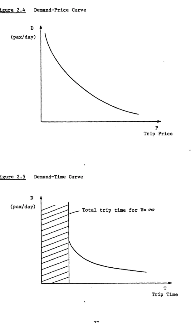
Traditionally, the "demand curve" is defined as the variation of

market demand with price (Figure 2.4). A demand curve can also be shown as a function of total trip time (Figure 2.5). In this case there is a number of components of total trip time. It should be noticed that decreasing the

flight time by increasing the cruise speed to an infinite value will not

make the total trip time zero.

demand-Figure 2.4 Demand-Price Curve

D

I

Figure 2.5 Demand-Time Curve

D

(pax/day)

Total trip time for V= 00

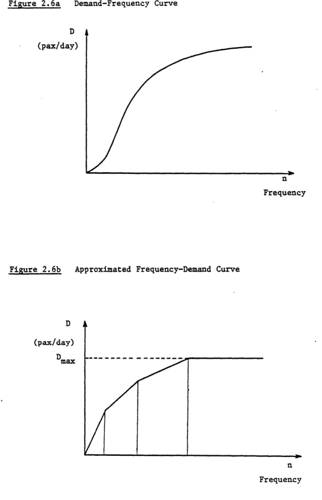
frequency curve (Figure 2.6a). Frequency becomes an important decision variable when airline competition exists. Independent of any postulates about the form of the demand model, it must be intuitively expected that a

demand-frequency curve of the form shown in figure 2.6a will exist. At a

frequency equal to zero, the demand must be zero. As the demand increases,

demand can be expected to increase until, at some large frequency, demand will saturate. That is, no matter how many more flights are added, demand will no longer increase; it has reached a saturation point. This due to the fact that adding one more frequency virtually does not reduce the

waiting time and therefore, makes no difference to the passenger.

A frequency elasticity, an, now exists that decreases when n is

increased: OD D n

[8D

r8

-t /n

As n ->w , e, -> 0, or saturation takes place.

The shape of the demand-frequency curve depends strongly upon the

time elasticity of demand, $, and the total trip time, T.

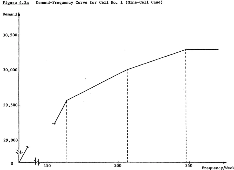
As mentioned earlier, the solution to the cell fleet planning problem is. found by means of solving a linear programming problem. The demand-frequency curves provide the "feasible region" necessary to solve

Figure 2.6a Demand-Frequency Curve

D

(pax/day)

Frequency

Figure 2.6b Approximated Frequency-Demand Curve

D

(pax/day)

Dmax ~~~ ~ ~~~ ~ ~

the problem. The curve shown in figure 2.6a obviously does not follow the

requirements of convexity and linearity necessary to form a linear programming problem's feasible region. Figure 2.6b shows the approximation

of the curve used in the Cell Fleet Planning Model. The curve is

linearized over a certain number of intervals. Each interval starts and ends at a "breakpoint" defined by a given frequency and its corresponding demand.

2.3 Mathematical Structure of the Cell Fleet Planning Model

A Linear Programming formulation consisting of the objective

function and seven constraints is used to solve the cell fleet planning

problem . These are now presented.

2.3.1 Objective Function

The objective is to maximize the not present value of profits. Profits are defined as the total operating revenues less the direct and

indirect operating costs and the cost of purchasing new aircraft.

Maximize Zt = I Z(t) t (REV/PA-I*NSEGc*PAXc) Z(t) - Operating c (1+RDISC) Revenues (COST/Flightc *NSEG*nc ) - vt 1t t Operating c v (1+RDISC)tl Costs

Cost of Ownership(IV _{vt+GI vt}

- t Aircraft

v

where:

a = cell

t = period of time (year) v- aircraft type (vehicle)

REV/PAXlc = revenue per passenger for cell c for year t

NSEGct = number of segments in cell c in year t

PAX c = number of passengers per day per segment in cell c in year t

COST/Flightvtc = cost per flight using aircraft v in cell c in year t

ncvt = number of flights per day using aircraft v in cell c in year t (frequency)

IV, = number of aircraft of type v in inventory at t=1 less the

aircraft v retired from year 1 to year t

GIvt = number of aircraft of type v purchased between years 1 and t RDISC = discount rate

2.3.2 Constraints

2.3.2.1 Demand Carried:

The total number of seats supplied over all intervals of the demand-frequncy curve for cell c in year t must satisfy the forecasted

number of passengers for that cell and year. Supplied number of seats will depend on the number of flights per day on each segment.

I S *NK t - PAX 1 0 k

for all a and t, where:

k = interval in demand-frequency curve

t = slope (seats per day per route segment) for cell c in year t lt = frequency at interval k (flights per day per segment) for

cell c in year t

PAXI = number of passengers in cell c in year t

2.3.2.2 Sum of Frequencies:

The sum of frequencies for all aircraft types for a given cell c and year t must be equal to the sum of frequencies for all intervals in

the demand-frequency curve for that cell a and year t.

n~t - I Kt 0

v k

for all c and t.

2.3.2.3 Load Factor:

The total capacity supplied by all aircraft types in a given

cell a and year t, taking into consideration load factors, must satisfy

the number of passengers for that cell and year.

SLyv *Cv * - PAXc > 0 v

LFV = load factor for aircraft type v Cv = seat capacity on aircraft type v

c

"1t - number of flights using aircraft type v on cell c in year t (frequency)

2.3.2.4 Frequency Range:

The number of flights per day in cell c and year t can be constrained by lower and upper bounds.

LLO < noe < LIO

for all c and t, where:

LLc _t = minimum number of flights in cell a and year t

ULc = maximum number of flights in cell c and year t

2.3.2.5 Fleet Utilization:

The total hours flown for aircraft type v in the system must

not exceed the maximum for that aircraft type.

1 (Thc * NSEGO * nc) _{t vt} Uvtax _tt (Ivt + GIvt) < 0

for all v and t, where:

Th = block time for cell c

NSEGc = number of segments in cell c in year t

nt ='number of flights with aircraft v in cell c and year t

vt

IVVt = number of aircraft of type v in inventory at t=1 less the aircraft v retired from year 1 to year t

GIvt - number of aircraft of type v purchased between years 1 and t

2.3.2.6 Fleet Continuity:

i) Continuity for Inventory Aircraft:

The number of aircraft of type v retired in year t must be equal to the number of aircraft v in inventory at the end of year t

less the number of aircraft v in inventory at the end of the previous

year. BP3>

Ivt ~ v(t-1) + R, = 0

for all v and t, where:

IVvt = number of aircraft v at the end of year t

IVv(t1) = number of aircraft v at the end of year t-1

t = number of aircraft of type v retired during year t

ii) Continuity for Gap Vehicles:

The number of aircraft of type v purchased in year t must

be equal to the number of aircraft of type v in the gap inventory at the

end of year t less the number of aircraft of type v in the gap inventory at the end of the previous year. The gap inventory is defined as the

GIvt - GIV(t-1) _- GVvt = 0 for all v and t, where:

GIvt = number of aircraft of type v purchased until the end of year t

- number of aircraft of type v purchased until the end of year t-1

CHAPTER 3.

INDUSTRY'S FLEET COMPOSITION IN RECENT YEARS

This chapter presents the composition of the U.S. airline industry's fleet bver the last five years, from 1979 to 1983. It is important to look at this data because it provides a clear picture of the

current industry's fleet structure, shows actual trends and serves as a

basis for comparison to the forecast generated by the Cell Fleet Planning

Model and to other forecasts. It is also interesting to analyze these

figures because the data corresponding to these five years, 1979 through 1983, is the data used to form the clusters (cells) and the demand-frequency curves described in Chapter '2 upon which the Cell Fleet

Planning Model is based.

Only large jet aircraft with capacity of 100 seats or more have been considered on the tables presented since those are the aircraft types included in this fleet planning case study (the smallest types

considered are DC9's and B737's). They are presented in two ways: by

individual aircraft type and by aircraft group. The generic groups considered are: wide-bodied, 4-engine; narrow-bodied, 4-engine; wide-bodied, 3-engine; narrow-wide-bodied, 3-engine; wide-bodied, 2-engine; and narrow-bodied, 2-engine aircraft. Table 3.1 shows the aircraft types

pertaining to each of the six groups.

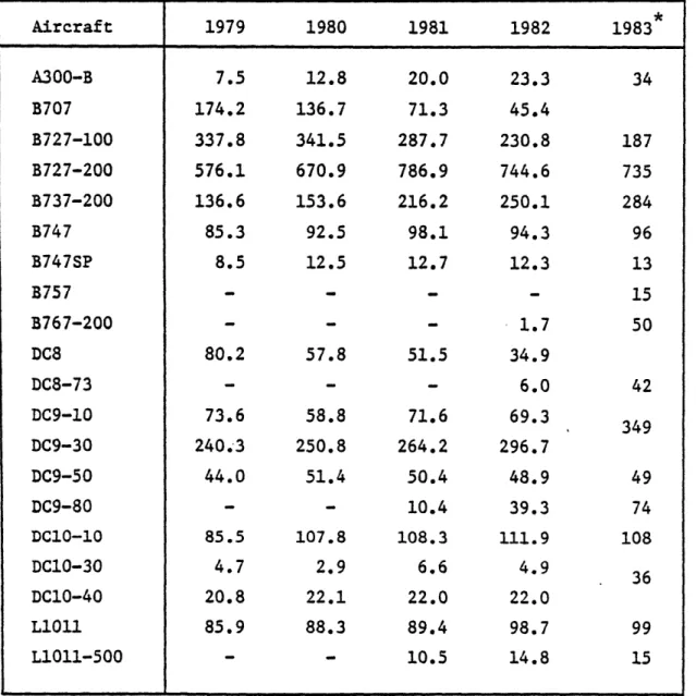
In table 3.2 the average number of aircraft assigned to service

from 1979 to 1982 for each individual type is shown.1

Composition of Aircraft Groups WIDE-BODIED, 4-ENGINE: B747 NARROW-BODIED, 4-ENGINE: B707 DC8 (all series) (all series) WIDE-BODIED, 3-ENGINE: DC10 (all L10ll (all series) series) NARROW-BODIED, 3-ENGINE: B727 (all series) WIDE-BODIED, 2-ENGINE: A300-B B767 NARROW-BODIED, 2-ENGINE: B737 - (all series) B757 DC9 (all series) I P1 I, Table 3. 1

Table 3.2 Average Number of Aircraft Assigned to Service Per Individual Type

*

Source for 1983 data: Aviation Daily, "Majors, Nationals Fleets"

Aircraft 1979 1980 1981 1982 1983 A300-B 7.5 12.8 20.0 23.3 34 B707 174.2 136.7 71.3 45.4 B727-100 337.8 341.5 287.7 230.8 187 B727-200 576.1 670.9 786.9 744.6 735 B737-200 136.6 153.6 216.2 250.1 284 B747 85.3 92.5 98.1 94.3 96 B747SP 8.5 12.5 12.7 12.3 13 B757 - - - - 15 B767-200 - - - 1.7 50 DC8 80.2 57.8 51.5 34.9 DC8-73 - - - 6.0 42 DC9-10 _{73.6 58.8 71.6} 69.3 ₃₄₉ DC9-30 240.3 250.8 264.2 296.7 DC9-50 44.0 51.4 50.4 48.9 49 DC9-80 - - 10.4 39.3 74 DC10-10 85.5 107.8 108.3 111.9 108 DC10-30 _{4.7 2.9 6.6} 4.9 36 DC10-40 20.8 22.1 22.0 22.0 L1011 85.9 88.3 89.4 98.7 99 L1011-500 - - 10.5 14.8 15

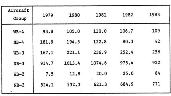
Table 3.3 presents the average number of aircraft assigned to

service aggregated into the six groups mentioned above.

In analyzing table 3.3 it is interesting to note that some aircraft

groups remain relatively stable while others -show a steady increase or

decrease. The group corrresponding to narrow-bodied, 4-engine aircraft is

steadily decreasing its number of aircraft. This constitutes no surprise since the group is formed by B707's and DC8's which are being phased out due to their old age and inefficiency compared to new aircraft, and to noise restrictions. The DC8-73, a re-engined version of the DC8-62, is an

exception to this group as can be seen in table 3.2.

Three groups that grew regularly during this period were the

wide-bodied, 3-engine, and wide-bodied and narrow-bodied, 2-engine groups. Until 1981 the wide-bodied, 2-engine groups was formed solely by the

increasing number of Airbuses (A300-B's). In 1982 the B767 was intioduced and then accounted for a small percentage of aircraft in this group. The increase in the narrow-bodied, 2-engine group is due mainly to the increasing number of B737-200's and DC9-30's and to the introduction of the DC9-80 in 1981 (table 3.2). The growing number of DC10-10's and

L1011's and the introduction of L1011-500's in 1981 are responsible for

the increase of the wide-bodied, 3-engine group.

Aeronautics Board Aircraft Operating Costs and Performance Reports. The

average number of aircraft assigned to service for each type is the sum of

majors and regionals international and local service domestic operations. The 1984 C.A.B. report which contains 1983 data is not available as of

this date. Data for 1983 included in tables 3.2 and 3.3 comes from a different source and may not be consistent with the C.A.B. data.

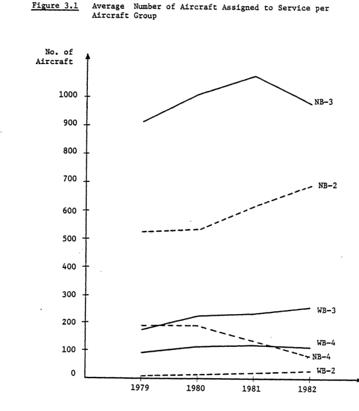
Table 3.3 Average Number of Aircraft Assigned to Service per Aircraft Group

where:

WB-4: wide-bodied, 4-engine aircraft NB-4: narrow-bodied, 4-engine aircraft WB-3: wide-bodied, 3-engine aircraft NB-3: narrow-bodied, 3-engine aircraft WB-2: wide-bodied, 2-engine aircraft NB-2: narrow-bodied, 2-engine aircraft Aircraft Group 1979 1980 1981 1982 1983 WB-4 93.8 105.0 110.0 106.7 109 NB-4 181.9 194.5 122.8 80.3 42 WB-3 167.1 221.1 236.9 252.4 258 NB-3 914.7 1013.4 1074.6 975.4 922 WB-2 7.5 12.8 20.0 25.0 84 NB-2 524.1 532.3 621.3 684.9 771

The wide-bodied, 4-engine group composed of B747's and the

narrow-bodied, 3-engine group composed of B727's (the most popular jet aircraft in commercial aviation history), did not show a defined increasing or decreasing pattern as did the other groups during these four years. They

both show a reduction in number of aircraft in 1982 after having increased during the previous three years.

Figure 3.1 plots the variation in the number of aircraft in each

group over the period of time extending from 1979 to 1982.

Given the availability of the clustring program and the OAG data for 1979 through 1983 which are used in the Cell Fleet Planning Model, historical data from the frequency point of view is now presented. These

figures will be useful in the analysis on the Cell Model results since

these include frequency-related data.

The clustering program enables us to determine which segments of the OAG data fall into each of nine cells as described in Chapter 2. Nine cells are used because for each of the three attributes of each cell

(frequency, distance, and seat volume) the possibility of them being high,

low, or medium in magnitude is considered. This gives 3x3=9 possible

combinations of attributes which result in the nine cells being used. . Each segment record contains information on the three attributes which define its corresponding cell and the frequency flown with each aircraft type on that segment. By means of simple Fortran computer programs the total frequency for each and all of the aircraft types flown

on the same cell has been aggregated. The present study focuses on the large jet aircraft listed in table 3.2, therefore, table 3.4 presents the daily frequency flown by each of these selected aircraft types aggregated

Figure 3.1 _{Average Number of Aircraft Assigned to Service per} Aircraft Group No. of Aircraft 1000 900 -800 -700 . 600 -500 -400 -300 -200 + 100 -0 1979 1980 1981 NB-3 - NB-2 WB-3 WB-4 NB-4 -.... ... .. --..- -- - - - --- -...- -- WB-2 1982

Br Qz E TZn ODS-ITOTfi CL 8c 9t StcZGTOrI CEt' 9st M Lrt' rcV 0To 00t, rUr S9 -08-63c tty901 009 TES 1T8V 0S-60a O1Z 9ZZ VT'6T E88T 0OUT 0C-63a CBS 69S ULS TES 6i4' oT-6ocI E91 SST L8T 68T 8ir

oL'09-8Zoa

TS

TZ

zzv

E

4:~~

_{V *}

shows this daily frequency for every cell throughout the five years. Appendix A.3 presents the complete list of aircraft and their frequencies

on each cell, which includes from B747's to small propeller aircraft.

Analyzing Table 3.4 it may be seen that the aircraft types that increased their daily frequencies are the A300-B, B737-200, DC9-30, and DC9-80. The DC9-80 was introduced in 1981. Other two aircraft types introduced during these five years were the B757 and B767-200, that were

put into service in 1983. Some aircraft types decreased their total number of daily frequencies: the B707, B727-100, and DC8. These frequency figures

correlate with the decreasing number of aircraft shown in Table 3.2. Aircraft types such as the B727-200, B737-100, B747, B747SP, DC10, and L1011 showed variations in their total daily frequencies throughout the

five years, but showed no defined trends.

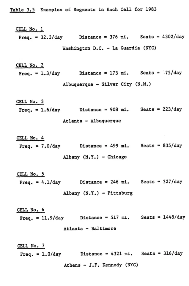
The attributes for each cell shown in Appendix A.1 correspond to daily figures per individual segment. (In table 3.5 some examples of

segments pertaining to each of the nine cells for 1983 are shown to

provide a concrete insight of the cells and their attributes.) The "daily

frequency" listed is the total number of flights per day with the given aircraft type over all segments in that cell. The "% of total cell frequency" corresponds to the percentage of the total number of

frequencies of that cell flown by each of the aircraft types. It should be

noted that these percentages do not add 100% since only selected aircraft types are listed. Should all types shown in Appendix A for each cell had

been listed, the sum would have resulted in 100%.

The "% of total type frequency" is the percentage of the total number of frequencies flown by that aircraft type in that year on that

Table 3.5 Examples of Segments in Each Cell for 1983

CELL No. 1

Freq. = 32.3/day Distance = 376 mi. Seats = 4302/day Washington D.C. - La Guardia (NYC)

CELL No. 2

Freq. = 1.3/day Distance = 173 mi. Seats = 75/day Albuquerque - Silver City (N.M.)

CELL No. 3 Freq. = 1.6/day CELL No. 4 Freq. = 7.0/day Distance = 908 mi. Atlanta - Albuquerque Distance = 499 mi. Seats = 223/day Seats = 835/day Albany (N.Y.) - Chicago

CELL No. 5

Freq. = 4.1/day Distance = 246 mi. Seats = 327/day

Albany (N.Y.) - Pittsburg

CELL No. 6

Freq. = 11.9/day Distance = 517 mi. Seats = 1448/day Atlanta - Baltimore

CELL No. 7

Freq. = 1.0/day Distance = 4321 mi. Seats = 316/day Athens - J.F. Kennedy (NYC)

Table 3.5 (cont.)

CELL No. 8

Freq. = 16.3/day Distance = 736 mi. Seats = 2627/day Boston - Chicago

CELL No. 9

Freq. = 1.6/day Distance = 1888 mi. Seats = 291/day Hartford - Dallas/Fort Worth

year is equal to 100%. The word frequencies should be emphasized since it

must be noted that percentage of frequencies is not equal to percentage of number of aircraft due to utilization and stage length considerations.

Furthermore, aircraft are not allocated to just a single cell; they are

flown on more than one cell.1

The lower portion of the tables in Appendix A.1 shows the

aggregation of the aircraft types into each of the six groups defined earlier. The total daily frequency and the percentage of the total

frequencies in the cell flown by a given aircraft group are presented. One must be very careful in comparing cells through the five years

since it must be noticed that two cells having the same number do not

necessarily have similar attributes. This is due to the different characteristics of data corresponding to each of the five years which results in a different clustering scheme. As an example take the cell which has as attributes a distance greater than 4000 miles, a frequency of

approximately one flight per day, and a seat volume of approximately 300

per day. These attributes are found in cell 3, cell 3, cell 5, cell 6, and cell 7 in years 1979 through 1983 respectively. Fortunately this problem

does not appear when analyzing the results of the Cell Fleet Planning Model in Chapter 5 since a matching of cells is performed as part of the

overall process.

Table 3.6 presents the total number of frequencies per aircraft

1For example consider the case of an airplane flying the route Boston-New

York-Madrid. The Boston-New York and New York-Madrid legs of the flight fall into different cells but the same aircraft is used.

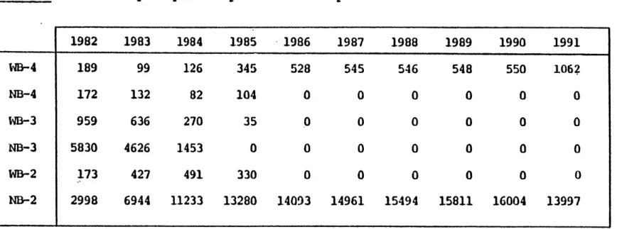
Daily Frequencies per Aircraft Group 1979 1980 1981 1982 1983 WB-4 229 238 230 234 227 NB-4 851 589 397 270 203 WB-3 789 799 854 852 844 NB-3 5887 5607 5765 5040 4987 WB-2 38 70 77 107 294 NB-2 4300 4143 4456 5892 6333 Table 3. 6

group from 1979 to 1983. These figures result from the aggregation over

all cells of the frequencies shown in tables 3.4.

Performing an analysis similar to that of table 3.3 it can be seen that the wide- and narrow-bodied, 2-engine aircraft groups show an increasing trend regarding the total number of frequencies. The narrow-bodied, 3- and 4-engine groups have decreased their total number of flights while the wide-bodied, 3- and 4-engine groups have remained

relatively stable.

Let us now compare table 3.6 against table 3.3, that is, the number of frequencies per aircraft group versus the actual number of aircraft assigned to service. The decrease in frequencies for the narrow-bodied,

4-engine aircraft group is a direct consequence of the reduction in the number of airplanes (DC8's and B707's) mentioned in the description of

table 3.3. The increasing trend in number of frequencies for the wide- and

narrow-bodied, 2-engine aircraft matches their trend for the number of airplanes assigned to service and therefore explains it. There is also consistency in the trends followed by the frequencies and number of

aircraft in the wide-bodied, 4-engine group (B747's).

In the case of the wide- and narrow-bodied, 3-engine aircraft some

discrepancy is found in their trends regarding number of frequencies and

number of aircraft. The number of wide-bodied, 3-engine aircraft increased

during the period while the total frequencies did not follow the upward pattern and remained approximately constant. For the narrow-bodied, 3-engine aircraft (B727's) the number of aircraft shows no defined trend

while its frequencies show decrease. The explanation for these

discrepancies is found in the frequency per cell data of Appendix A.1:

narrow-bodied, 3-engine aircraft, DC10's, L1011's, and B727's, to longer range routes. In other words, the number of frequencies for these airplanes tends to increase in cells with larger distance attribute while it tends

to decrease in those cells with shorter distance. With similar utilizations, if the average stage length for these aircraft is increased,

the total number of frequencies has to decrease.

The frequency-related data presented in this chapter (table 3.4 and

3.6 and Appendices A) could be very useful in future studies concerning

the routes and structure of the U.S. airline industry. Results of the Fleet Planning Model provide data in this form and Chapter 5 refers to the

model's results and to the historical data of the present chapter in its

CHAPTER 4.

APPLICATION OF THE CELL FLEET PLANNING MODEL: A CASE STUDY

This chapter presents an application of the Cell Fleet Planning Model to an industry-wide scenario. This is from the stand point of a manufacturer, who in his long term planning is not concerned with individual airlines or group of airlines or even regions, but is interested in forecasting the total number of aircraft that will be needed. This is equally true in the case of airframe manufacturers, such as Boeing, McDonnell Douglas, and Airbus, as in the case of engine

manufacturers such as Pratt & Whitney, General Electric, and Rolls Royce. Four runs of the Model have been performed: three considering nine cells and another considering thirty cells. The three nine-cell cases considered, case A, case B, and case C, include three different scenarios. Two of these cases, A and B, use the same input data, but case

B was run with a slight modification to the Cell Fleet Planning Model1; in case B the Model is forced to utilize the aircraft it has available each year of the planning period. As will be seen in the outputs, this

will result in a higher overall utilization of inventory aircraft and in

less aircraft purchases. In cases A and C, the Model has the freedom of grounding some of its inventory aircraft which it considers inefficient

1In case B, the Fleet Utilization Constraint (Section 2.3.2.5) has been changed from a "less than or equal" relationship to an equality. This forces the aircraft in inventory to be utilized since the total hours

or not optimal to be flown. The scenario in case C shows two changes with

respect to cases A and B: i)the maximum number of aircraft available for each year some aircraft types has been constrained to a higher degree than in cases A and B, to reflect the scenario of a slower production rate by the manufacturers or a lesser purchase capability by the airlines; and, ii) the minimum number of aircraft for each year has been

relaxed for some aircraft types (e.g. B727-200) to reflect the case of a

higher rate of retirements. This is done through the Maximum and Minimum

Fleet Count by Type by Year Table (Section 4.2.9). The reason for using nine cells and the procedure for determining an *optimal' number of cells, thirty, have been described in Chapter 2. One of the objectives of

this thesis is to compare the results obtained for these two cases. This

is done in Chapter 5. Sections 4.2 and 4.3 describe and present respectively the actual inputs and outputs for the nine-cell and thirty-cell cases.

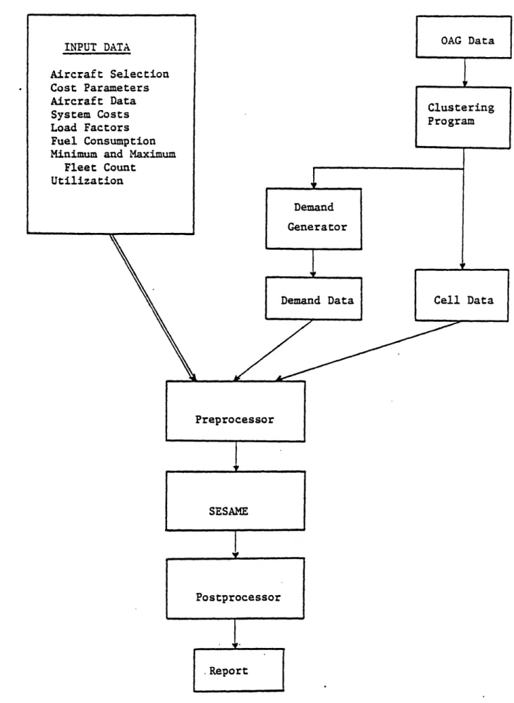
4.1 Computer Implementation of the Cell Fleet Planning Model

A flowchart describing the computer implementation of the Cell

Fleet Planning Model is shown in Figure 4.1. It consists of ten input

tables, a demand generator program, the clustering programs, a

preprocessor, a Linear Programming package, and a postprocessor.

As mentioned earlier, the cell fleet planning problem is formulated

as a Linear Programming problem, and, it is solved by means of a standard

software package. Currently the Model is loaded on M.I.T.'s IBM 3031

system and the Linear Programming package used is SESAME, an M.I.T.

equivalent of IBM's MPSX.

Figure 4.1 Flowchart of the Cell Fleet Planning Model INPUT DATA Aircraft Selection Cost Parameters Aircraft Data System Costs Load Factors Fuel Consumption

Minimum and Maximum

Fleet Count Utilization

the input tables and build the objective function and constraints of the Model. The output of this preprocessor is a standard matrix which constitutes the input to SESAME. The input tables are described in the

following section.

The output from SESAME is a matrix containing the optimal solution values for the decision variables. The function of the postprocessor is

to read these values and build an output report as the ones shown and

described in Section 4.3.

4.2 Inputs

Different types of data are required as inputs to the Cell Fleet

Planning Model, such as aircraft operating and cost data, financial data,

demand data, etc. Most of the aircraft-related input data used here was provided by Pratt & Whitney who is the principal industry supporter of

this study within the framework of a Cooperative Research Program between M.I.T. and the industry. Pratt & Whitney is a member of this consortium.

Ten input tables or files exist. These are now described.

4.2.1 Aircraft Selection Table

This table contains the aircraft types to be considered in the run of the Model. In the present case, thirty-one types have been

considered. They are all large jet aircraft and include the airplanes

built by the leading manufacturers and most used by airlines all over the

world. Some non-existing aircraft types have also been included to

reflect possible new aircraft appearances during the planning term. These types are the B150, B767-3, B767-XI, F100, and TA11.