Applying Engineering and Fleet Detail to
Represent Passenger Vehicle Transport in a
Computable General Equilibrium Model
Valerie J. Karplus, Sergey Paltsev, Mustafa Babiker,
John Heywood and John M. Reilly
The MIT Joint Program on the Science and Policy of Global Change is an organization for research, independent policy analysis, and public education in global environmental change. It seeks to provide leadership in understanding scientific, economic, and ecological aspects of this difficult issue, and combining them into policy assessments that serve the needs of ongoing national and international discussions. To this end, the Program brings together an interdisciplinary group from two established research centers at MIT: the Center for Global Change Science (CGCS) and the Center for Energy and Environmental Policy Research (CEEPR). These two centers bridge many key areas of the needed intellectual work, and additional essential areas are covered by other MIT departments, by collaboration with the Ecosystems Center of the Marine Biology Laboratory (MBL) at Woods Hole, and by short- and long-term visitors to the Program. The Program involves sponsorship and active participation by industry, government, and non-profit organizations.
To inform processes of policy development and implementation, climate change research needs to focus on improving the prediction of those variables that are most relevant to economic, social, and environmental effects. In turn, the greenhouse gas and atmospheric aerosol assumptions underlying climate analysis need to be related to the economic, technological, and political forces that drive emissions, and to the results of international agreements and mitigation. Further, assessments of possible societal and ecosystem impacts, and analysis of mitigation strategies, need to be based on realistic evaluation of the uncertainties of climate science.
This report is one of a series intended to communicate research results and improve public understanding of climate issues, thereby contributing to informed debate about the climate issue, the uncertainties, and the economic and social implications of policy alternatives. Titles in the Report Series to date are listed on the inside back cover.
Ronald G. Prinn and John M. Reilly Program Co-Directors
For more information, please contact the Joint Program Office
Postal Address: Joint Program on the Science and Policy of Global Change 77 Massachusetts Avenue
MIT E19-411
Cambridge MA 02139-4307 (USA)
Location: 400 Main Street, Cambridge
Building E19, Room 411
Massachusetts Institute of Technology
Access: Phone: +1.617. 253.7492
Fax: +1.617.253.9845
E-mail: globalchange@mit.edu
Web site: http://globalchange.mit.edu/
Applying Engineering and Fleet Detail to Represent Passenger Vehicle Transport in a Computable General Equilibrium Model
Valerie J. Karplus*,†, Sergey Paltsev*, Mustafa Babiker*, John Heywood‡ and John M. Reilly*
Abstract
A well-known challenge in computable general equilibrium (CGE) models is to maintain correspondence between the forecasted economic and physical quantities over time. Maintaining such a correspondence is necessary to understand how economic forecasts reflect, and are constrained by, relationships within the underlying physical system. This work develops a method for projecting global demand for passenger vehicle transport, retaining supplemental physical accounting for vehicle stock, fuel use, and greenhouse gas (GHG) emissions. This method is implemented in the MIT Emissions Prediction and Policy Analysis Version 5 (EPPA5) model and includes several advances over previous approaches. First, the relationship between per-capita income and demand for passenger vehicle transport services (in vehicle-miles traveled, or VMT) is based on econometric data and modeled using quasi-homothetic preferences. Second, the passenger vehicle transport sector is structured to capture opportunities to reduce fleet-level gasoline use through the application of vehicle efficiency or alternative fuel vehicle technologies, introduction of alternative fuels, or reduction in demand for VMT. Third, alternative fuel vehicles (AFVs) are introduced into the EPPA model. Fixed costs as well as learning effects that could affect the rate of AFV introduction are captured explicitly. This model development lays the foundation for assessing policies that differentiate based on vehicle age and efficiency, alter the relative prices of fuels, or focus on promoting specific advanced vehicle or fuel technologies.
Contents
1. INTRODUCTION ... 2
2. BOTTOM-UP TECHNOLOGY IN TOP-DOWN MODELS ... 3
2.1 Background on the CGE Modeling Approach ... 3
2.2 A Literature Review on Approaches to Modeling Energy-intensive Durable Goods ... 3
2.3 A Strategy for Modeling Passenger Vehicle Transport in a CGE Framework ... 5
2.4 Summary of Modeling Approach ... 7
3. DESCRIPTION OF NEW MODEL DEVELOPMENTS ... 8
3.1 Development 1: Income Elasticity of Demand for Vehicle Travel in a CGE Framework . 8 3.1.1 Income Elasticity of Demand for VMT: Empirical Evidence ... 9
3.1.2 Forecasting Passenger Vehicle Transport Services in a CGE Framework ... 10
3.1.3 Implementing Income Elasticity of Demand as a Function of Per-capita Income ... 12
3.2 Development 2: Modeling Opportunities for Vehicle Efficiency Improvement ... 16
3.2.1 Opportunities for Vehicle Efficiency Improvements: New Sector Structure ... 16
3.2.2 Modeling Fleet Turnover Using a Two-vintage Approach ... 17
3.2.3 Fuel Efficiency Response to Fuel Price in New Passenger Vehicles ... 18
3.3 Development 3: Representation of Alternative Fuel Vehicles... 21
3.3.1 Parameterization and Key Elasticities ... 22
3.3.2 Constraints on Adoption ... 24
4. SENSITIVITY EXERCISES USING NEW MODEL DEVELOPMENTS... 24
5. SUMMARY AND EXTENSIONS ... 26
3. REFERENCES ... 26
*
MIT Joint Program on the Science and Policy of Global Change, Cambridge, MA.
† Corresponding author: MIT Joint Program on the Science and Policy of Global Change. 400 Main Street, Building E19, Room 429p, Cambridge, MA 02139-4307(E-mail: vkarplus@mit.edu).
1. INTRODUCTION
Computable general equilibrium (CGE) models are widely used to understand the impact of policy constraints on energy use, the environment, and economic welfare at a national or global level (Weyant & Hill, 1999; U.S. CCSP, 2007). However, for certain research questions, results from these models can produce misleading forecasts if they do not capture accurately the relationships in the underlying physical system. These relationships include links between income and demand for services provided by energy-intensive durable goods, as well as the richness of opportunities for technological or behavioral change in response to policy.
Maintaining dual accounting of physical and economic variables is particularly important when modeling consumer durable goods such as passenger vehicles. Vehicles are an example of a complex multi-attribute consumer product with a long lifetime. Consumer preferences across attributes—such as horsepower and fuel economy in the case of vehicles—involve engineering trade-offs at the vehicle level. For instance, over the past several decades, fuel efficiency gains have been offset by a shift toward larger, more powerful vehicles in some regions, offsetting improvements in on-road fuel economy (An & DeCicco, 2007). As policymakers consider how to most cost-effectively regulate the air, climate, and security externalities associated with vehicle use, macroeconomic forecasting models that capture the range of technological and behavioral responses to regulation will become increasingly important.
The goal of this work is to develop a new method of projecting physical demand for services from passenger vehicles in a recursive-dynamic CGE model. This new method is applied to the MIT Emissions Prediction and Policy Analysis (EPPA) model, a CGE model of the global economy (Babiker et al., 2001; Paltsev et al., 2005; Paltsev et al., 2010). The method captures the richness of the technological response at an appropriate level of detail, without sacrificing sectoral and regional coverage or the ability to capture the macroeconomic feedbacks that make this modeling system advantageous over other approaches.
The text is organized as follows. Section 2 identifies the shortcomings of current practices for representing energy-intensive consumption at the household level in CGE models, including the representation of durable goods, and the rationale for a new approach. Section 3 presents the new approach, divided into three parts. Section 3.1 explains how the relationship between income and demand for vehicle services was parameterized using econometric information and implemented using the well-established Stone-Geary (quasi-homothetic) preference system. Section 3.2 describes how vehicle engineering and fleet detail were used to parameterize the structure of the passenger vehicle transport sector and opportunities for fleet-level fuel efficiency improvement. Section 3.3 describes the representation of alternative fuel vehicles. Section 4 describes the impact of model developments on forecasts of gasoline use, greenhouse gas (GHG) emissions, and household consumption. Section 5 offers conclusions and directions for future work.
2. BOTTOM-UP TECHNOLOGY IN TOP-DOWN MODELS 2.1 Background on the CGE Modeling Approach
The CGE model structure is based on the circular flow of the economy in which households supply labor and capital to firms that produce goods and services, which are in turn purchased by households. The CGE model has its origins principally in neoclassical modeling developments and invokes microeconomic principles (Arrow & Debreu, 1954; Shoven & Whalley, 1984). Based on their endowments and preferences, one or more representative agents maximize utility subject to a budget constraint, while producers maximize profits, with production functions specified as constant returns-to-scale. A vector of prices and quantities for which demand equals supply (market clearance), household income equals expenditures (income balance), and the profits of firms are driven to zero (zero profit) comprises an equilibrium solution. The basis for CGE model calibration is typically National Income and Product Account data, which is used to develop a Social Accounting Matrix (SAM) that captures economic flows across all sectors in a single model benchmark year. The SAM has its origins in traditional input-output (I/O) analysis (Leontief, 1937). Many CGE models are written in the GAMS software system and may be formulated in the MPSGE programming language (Rutherford, 1999).
In the structure of a CGE model, elasticities of substitution represent the willingness or ability of households and firms to substitute among inputs to production or consumption in response to changes in input costs. The elasticity values are typically based on econometric evidence or other methods as appropriate (Arndt et al., 2007; Balistreri et al., 2001; Zhang & Verikios, 2006). Most CGE models also include some form of capital stock accounting, either using a putty-clay representation (Phelps, 1963; Lau et al., 2002) or a sector-specific capital vintaging structure (Paltsev et al., 2005).
2.2 A Literature Review on Approaches to Modeling Energy-intensive Durable Goods
A perennial challenge in the CGE modeling community has been how to forecast both expenditures and physical quantities consistently. Expenditure shares and elasticities are parameterized based on physical quantities, prices, and abatement costs in the benchmark year and are expressed in value terms. Expressing a quantity in value terms means that the benchmark year quantity is defined as the price multiplied by the quantity in that year and prices are
normalized to unity. In future model years, however, pinning down the relationship between spending, goods purchased, as well as the impact on demand for efficiency-improving
technologies can be difficult, since it requires assumptions about how these relationships will evolve over time. An example of the introduction of thermodynamic efficiency in CGE models can be found in McFarland et al. (2004).
The problems that arise from imprecise physical accounting can be particularly pronounced in the case of complex, quality-differentiated consumer durable goods because forecasted
expenditures must capture changes in demand for the service itself. The relationship between expenditures and service demand may change due to a variety of factors, including
attributes of the good that provides the services. Omitting such factors can produce misguided forecasts because the attributes of durable goods are defined in the benchmark year, and unless otherwise specified change only due to price-driven substitution among inputs. The total energy requirement may also be misestimated because tradeoffs between fuel economy and other product attributes are often not well specified. Functional attributes can be energy saving—i.e. technology that decreases fuel consumption per mile—or energy intensive—i.e. technology that increases fuel consumption per mile, or possibly have no net effect on fuel consumption at all. Forecasting energy requirements is difficult when the model does not resolve how income and input costs (including fuel cost) affect demand for vehicle services and product attributes, and its relationship to household spending.
Before describing the approach developed in this work, I briefly review the range of modeling approaches used to assess the impact of policy on consumption of energy-intensive durable goods. In developing models for energy and environmental policy analysis, researchers have tried various strategies to address the problem of how to simultaneously forecast physical and economic variables. One approach is to focus on the detailed physical system while holding exogenous macroeconomic variables (including in some instances prices) fixed, and forecast energy use (and technology adoption) using a cost minimization algorithm that takes policy, if imposed, as a constraint. By definition many macroeconomic models—including partial and general equilibrium models—encompass more than one market and capture the price changes that result from inter-market interactions. These models often sacrifice technological detail in the interest of generalizable insights and computational tractability, representing production and consumption activities in a deliberately simplified and aggregated fashion. Without additional structure it is impossible to determine, for instance, how demand for vehicle use responds to changes in the vehicle and fuel components of travel cost since these models only forecast the value of services provided.
One approach designed to preserve bottom-up technological detail without sacrificing macroeconomic feedbacks involves the coupling of highly aggregated macroeconomic models with detailed models of the physical system. An example for transport is the analysis by Schafer and Jacoby (2006), which coupled a top-down (CGE) model with a bottom-up (MARKAL) model and a mode share forecasting model to evaluate the impact of climate policy on
transportation mode shares and technology adoption. Other examples of this approach have been implemented for the electric power sector (Sue Wing, 2006) and for aggregated production and consumption activities in models (Messner & Schrattenholzer, 2000).
Still other models provide a system of fleet and fuel use accounting that forecasts the impact of individual technology scenarios (which are an input to the model). These scenarios may be carefully designed to achieve compliance with a particular policy target but do not typically capture the economic response. Models in this category include the Sloan Automotive Lab U.S. Fleet Model as well as the International Energy Agency’s global fleet model (Bandivadekar, 2008; Fulton & Eads, 2004).
However, all of these approaches—and the CGE approaches in particular—are not generally capable of tracking both the economic and physical variables simultaneously and consistently within a single model framework. Few existing CGE models treat passenger vehicle transport explicitly in household consumption.
2.3 A Strategy for Modeling Passenger Vehicle Transport in a CGE Framework
We develop a model of passenger vehicle transport that introduces constraints on forecasts of economic and physical variables by implementing a technology-rich model structure and
parameter calibration. The new model developments can be grouped into three categories, and are shown graphically in Figure 1.
First, the model captures how expenditures on passenger vehicle transport will change with per capita income, as consumers increase their vehicle holdings and travel more miles according to their travel needs. The income elasticity of demand for VMT has been shown to vary with per-capita income, geography, availability of substitute modes, and other factors. To account for this variation we estimate country or regional level income elasticities of demand for VMT. We implement these elasticities in the CGE framework using quasi-homothetic (Stone-Geary) preferences.
Second, we add new structure to the vehicle sector that separately describes miles traveled in new and used vehicles as well as the response of new vehicle fuel efficiency to fuel price
changes or policy mandates. These features are important because they allow the analysis of policies focused only on new vehicles, capture the impacts that technology adoption will have on the overall efficiency characteristics of the fleet, and reflect regional differences in average vehicle age, new vehicle investment, and vehicle retirement patterns. The new structure also captures the relationship between vehicle attributes and per-mile fuel consumption, as well as how per-mile fuel consumption of the fleet responds to changing fuel prices through demand response and investment in efficiency-improving technology.
Third, we represent opportunities for reducing GHG emissions and fuel consumption through the adoption of alternative fuel vehicles. Alternative fuel vehicles are then implemented to compete directly with the internal combustion engine (ICE)-only vehicle. These advanced “backstop” technologies are parameterized using current and future cost estimates based on engineering data and projections.
The model used to illustrate this three-part approach for the case of passenger vehicle
transport is the MIT Emissions Prediction and Policy Analysis (EPPA) model. The EPPA model is a recursive-dynamic general equilibrium model of the world economy developed by the Joint Program on the Science and Policy of Global Change at the Massachusetts Institute of
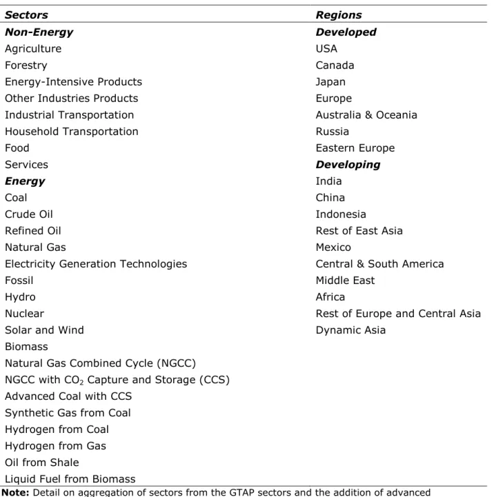
Technology (Paltsev et al., 2005). The EPPA model is built using the Global Trade Analysis Project (GTAP) dataset (Hertel, 1997; Dimaranan & McDougall, 2002). For use in the EPPA model, the GTAP dataset is aggregated into 16 regions and 24 sectors with several advanced technology sectors that are not explicitly represented in the GTAP data (Table 1). Additional data for emissions of greenhouse gases (carbon dioxide, CO2; methane, CH4; nitrous oxide, N2O; hydrofluorocarbons, HFCs; perfluorocarbons, PFCs; and sulphur hexafluoride, SF6) and air
pollutants (sulphur dioxide, SO2; nitrogen oxides, NOx; black carbon, BC; organic carbon, OC; ammonia, NH3; carbon monoxide, CO; and non-methane volatile organic compounds, VOCs) are based on United States Environmental Protection Agency inventory data and projects.
Table 1. Sectors and regions in the EPPA model.
Sectors Regions
Non-Energy Developed
Agriculture USA
Forestry Canada
Energy-Intensive Products Japan
Other Industries Products Europe
Industrial Transportation Australia & Oceania
Household Transportation Russia
Food Eastern Europe
Services Developing
Energy India
Coal China
Crude Oil Indonesia
Refined Oil Rest of East Asia
Natural Gas Mexico
Electricity Generation Technologies Central & South America
Fossil Middle East
Hydro Africa
Nuclear Rest of Europe and Central Asia
Solar and Wind Dynamic Asia
Biomass
Natural Gas Combined Cycle (NGCC) NGCC with CO2 Capture and Storage (CCS) Advanced Coal with CCS
Synthetic Gas from Coal Hydrogen from Coal Hydrogen from Gas Oil from Shale
Liquid Fuel from Biomass
Note: Detail on aggregation of sectors from the GTAP sectors and the addition of advanced
technologies are provided in Paltsev et al. (2010).
Much of the sectoral detail in the EPPA model is focused on providing a more accurate representation of energy production and use as it may change over time or under policies that limit greenhouse gas (GHG) emissions. The base year of the EPPA model is 2004, and the model is solved recursively in five-year intervals starting with the year 2005. The EPPA model
represents production and consumption sectors as nested Constant Elasticity of Substitution (CES) functions (or the Cobb-Douglas and Leontief special cases of the CES). The model is written in the GAMS software system and solved using MPSGE modeling language (Rutherford, 1995). The EPPA model has been used in a wide variety of policy applications (e.g., U.S. CCSP, 2007). Earlier development of this model disaggregated household vehicle transport and added detail to represent several types of alternative fuel vehicles (Paltsev et al., 2004; Sandoval et al., 2009; Karplus et al., 2010).
2.4 Summary of Modeling Approach
With the above challenge in mind, I develop a model of passenger vehicle transport that introduces constraints on forecasts of economic and physical variables by implementing a technology-rich model structure and parameter calibration. The new model developments can be grouped into three categories, and are shown graphically in Figure 1.
Figure 1. Schematic overview of the passenger vehicle transport sector incorporated into the representative consumer’s utility function of the MIT EPPA model. New
developments are highlighted on the right-hand side of the utility function structure.
First, the model captures how expenditures on passenger vehicle transport will change with per capita income, as consumers increase their vehicle holdings and travel more miles according to their travel needs. The income elasticity of demand for VMT has been shown to vary with per-capita income, geography, availability of substitute modes, and other factors. To account for this variation I estimate country- or regional-level income elasticities of demand for VMT. I
implement these elasticities in the CGE framework using quasi-homothetic (Stone-Geary) preferences.
Second, I add new structure to the vehicle sector that separately describes miles traveled in new and used vehicles as well as the response of new vehicle fuel efficiency to fuel price changes or policy mandates. These features are important because they allow the analysis of
policies focused only on new vehicles, capture the impacts that technology adoption will have on the overall efficiency characteristics of the fleet, and reflect regional differences in average vehicle age, new vehicle investment, and vehicle retirement patterns. The new structure also captures the relationship between vehicle attributes and per-mile fuel consumption, as well as how per-mile fuel consumption of the fleet responds to changing fuel prices through demand response and investment in efficiency-improving technology.
Third, I represent opportunities for reducing GHG emissions and fuel consumption through the adoption of alternative fuel vehicles. Alternative fuel vehicles are then implemented to compete directly with the internal combustion engine (ICE)-only vehicle. These advanced “backstop” technologies are parameterized using current and future cost estimates based on engineering data and projections.
The model used to illustrate this three-part approach for the case of passenger vehicle transport is the MIT EPPA model. The EPPA model represents production and consumption activities as Constant Elasticity of Substitution (CES) functions (or the Cobb-Douglas and Leontief special cases of the CES).4 Earlier development of this model disaggregated household vehicle transport and added detail to represent alternative fuel vehicles (Paltsev et al., 2004; Sandoval et al., 2009; Karplus et al., 2010).
3. DESCRIPTION OF NEW MODEL DEVELOPMENTS
The approach to modeling passenger vehicle transport is described here in a manner that is intentionally not specific to the MIT EPPA model. The goal is to provide an approach that can be easily adapted to a variety of CGE modeling environments. In instances where specific features of the EPPA model are involved, they will be explicitly described. The next three sub-sections provide a detailed description of the three-part modeling approach, working from top to bottom through the changes to the utility function described in Figure 1.
3.1 Development 1: Income Elasticity of Demand for Vehicle Travel in a CGE Framework
The objective of the first model development is to introduce an income elasticity of demand for vehicle transport services that differs by model region. In a CGE model the relationship between total household expenditures and spending on passenger vehicle transport is defined by an expenditure share, or the fraction of total expenditures devoted to services provided by passenger vehicles. Typically CGE models assume homothetic preferences, with the result that expenditure shares do not change as a function of income—in other words, the income elasticity of demand is equal to unity. For some goods—particularly goods that fulfill a basic need such as food, transport, or shelter—it is important to consider how this expenditure share will change as a function of income. Capturing this trend is important because in reality the expenditure share
4 Formulation as a Mixed Complementarity Problem in the Mathematical Programming Subsystem for General Equilibrium (MPS/GE) facilitates parsimonious model representation as well as provided an efficient solution method (Rutherford, 1999).
devoted to vehicle transport in a region is nonexistent or small when only a few households own vehicles, but grows as vehicle ownership comes within reach of an ever larger fraction of
households.
3.1.1 Income Elasticity of Demand for VMT: Empirical Evidence
To add empirical foundations to the new model structure, this work builds on previous studies that have attempted to measure how the household vehicle transport expenditure share and vehicle ownership vary over time and with per-capita GDP (Schafer & Victor, 2000; Meyer et
al., 2007; Dargay & Gately, 2007). Trends in vehicle ownership and the total household transport
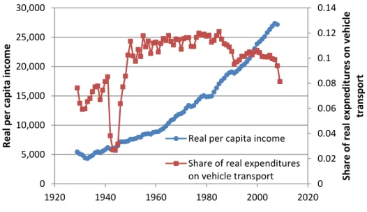
expenditure share5 in developed countries since the early twentieth century suggest that the expenditure share devoted to transport increases from 5% to 15% as vehicle ownership increases from zero to 200 cars per 1000 capita and then stays roughly constant thereafter (Schafer, 1998). Other studies have projected vehicle ownership using a Gompertz models (in which the
relationship between per-capita income and vehicle ownership is modeled with a sigmoid equation) as well as economic approaches based on empirical demand system estimation.6
Since this work focuses on the United States in a global context, significant effort was made to obtain the best available estimates of income elasticity of demand for vehicle-miles traveled using detailed U.S. data. The long-run rates of growth in spending on passenger vehicle
transportation and of growth in VMT in the United States are shown in Figure 2. Over the period considered (1970-2007), spending on passenger vehicle transportation increased at an average compounded growth rate of 3.86% per year, while VMT increased by 2.70% per year.7 The number of vehicles has grown at 2.27% per year, while growth in vehicle miles-traveled has averaged around 0.42% per year. This graph provides evidence that CGE models, which rely on exogenous gross domestic product (GDP) paths and fixed expenditure shares, are likely to underestimate or overestimate VMT growth if they do not consider explicitly how expenditure shares may changes with income.
5 The total household transport expenditure share includes expenditures on vehicle ownership as well as purchased transport modes, such as rail, road, aviation, and marine.
6 Dargay et al. (2007) estimates a model that relates per capita GDP to long-term income elasticities, and includes a term that accounts for a country-specific vehicle ownership saturation level. Meyer et al. (2007) compare projections using a Gompertz approach and a Stone-Geary based approach. In this study we are interested in the elasticity of demand for vehicle services (VMT), not only vehicle stock. If the number of miles-traveled per vehicle changes with per-capita income and vehicle stock, income elasticities of vehicle ownership may not be a good proxy for income elasticities of VMT demand.
7 Part of this discrepancy can be explained by an increase in average real vehicle price over the same period of around 2% per year (Abeles, 2004), which reflects the changes in the aesthetic and functional attributes of the vehicles themselves. A brief review of this trend is provided in the Supplementary Material.
Figure 2. Long-run trends in the growth of real expenditures on vehicle transport, VMT, vehicle ownership, gasoline usage, and miles-traveled per vehicle in the United States.
This observation is consistent with other empirical estimates of the income elasticity of
demand, which have been estimated to range from 0.3 (short run) to 0.73 (long run) (Hanly et al., 2002).8 This is reflected in the declining share of real expenditures on vehicle transport services, shown in Figure 3 (BEA, 2010).9
3.1.2 Forecasting Passenger Vehicle Transport Services in a CGE Framework
Calibrating the income elasticity of demand for transport services in a CGE model presents several challenges. CGE models assume a form of preferences that governs the consumption activities of households. The most common form, homothetic preferences, provides a clean and simple structure that requires minimal parameter assumptions.10 As mentioned, in this preference system, the shares of consumption activities in total spending are assumed to remain constant as income increases (expansion path through the origin with slope of unity).
8
This estimated income elasticity of demand for VMT represents the role of income as distinct from price (and other region-specific) effects.
9
It is worth noting here that the decline in expenditure share in 2008 and 2009 includes the effect of the economic crisis in 2008 and 2009, which may overstate the magnitude of the decline. Long-run estimates of the income elasticity of demand are used to calibrate CGE models, which typically resolve outputs in multi-year time steps. 10 The constant elasticity of substitution (CES) utility function (including the special case of the Cobb-Douglas
utility function) gives rise to homothetic preferences, which means that the ratio of goods demanded depends only on their relative prices, and not on the scale of production (constant returns to scale).
Figure 3. The share of real household expenditures on passenger vehicle transport has declined over the past 15 years (BEA, 2010).
Generically speaking, the problem is that many categories of expenditures—for example, food, clothing, and vehicles—do not increase uniformly with income, either in terms of the share of total consumption expenditures or in natural units.11 As a result, expenditures on passenger vehicle transport may not be tightly correlated with VMT beyond the base year, although historical evidence indicates that they tend to move in the same direction.12 The modeling challenge is to develop a structure that captures both changes in the underlying input prices (and thus cost of providing transport services) as well as changes in the income elasticity of demand for the service itself (in this case, VMT), which together determine the relationship between passenger vehicle transport expenditures and vehicle-miles traveled.
The cornerstone of this part of modeling strategy is a relationship defined in the benchmark year between spending on VMT (denoted here as - ) and the quantity of VMT in its natural units (denoted here as - ). The output of passenger vehicle transport in value terms over time can thus be interpreted using this benchmark year relationship, which is shown in Equation 1. In this equation, refers to the cost-per-mile of driving, which is used to determine - in the benchmark year. In each subsequent model period the expenditure share of - is determined using the income elasticity of demand, while underlying changes in input costs
and the substitution elasticities in region influence the price and level of output.
Substitution elasticities reflect how an increase in the price of one input results in compensating
11 In CGE models the energy-intensive activities that rely on an underlying capital stock are modeled in terms of the levelized cost of providing the service, assuming a time cost of money to obtain the rental value of capital across the full ownership horizon. This approach is described in detail for other sectors in the EPPA model in Paltsev et
al., 2005.
12 An extreme case might occur if consumers shifted spending to luxury vehicles but drove them far less often. 0 0.02 0.04 0.06 0.08 0.1 0.12 0.14 0 5,000 10,000 15,000 20,000 25,000 30,000 1920 1940 1960 1980 2000 2020 Sha re o f re al ex pn e dit ur es o n veh icl e tra ns po rt R e al pe r ca pit a inco m e
Real per capita income Share of real expenditures on vehicle transport
shifts to rely on other inputs, and the calibration of relevant elasticities is described later in Section 3.2.
- - (1)
Forecasted - can be calculated by dividing the value of sector output at each five-year interval by the cost-per-mile and the relative price of output (which has been normalized to unity in the base year). The number of vehicles on the road is calculated using the non-powertrain capital input, which provides an index for vehicle stock growth.
The main advantage of this method is that it allows the expenditure share to be determined uniquely in each five-year time step as a function of the income elasticity of demand for VMT (vehicle transport services). By defining the expenditure share in terms of - and
underlying cost per mile, the income elasticity of demand for VMT can be applied directly to capture changing demand for vehicle services (VMT), vehicles, and energy use. This improves on previous approaches, which often do not account for income-dependent variation in the vehicle transport budget share over time.13 The practical result of this approach, which I will describe in the following paragraphs, is to produce more realistic and empirically-based forecasts of spending on passenger vehicle transport services over time.
3.1.3 Implementing Income Elasticity of Demand as a Function of Per-capita Income In order to implement this approach in a CGE framework, a different, quasi-homothetic preference relationship is used to define the household utility function and demand for passenger vehicle transport services—implemented at the level of the top (red) box in Figure 1—to allow the calibration of an income elasticity of demand for VMT that differs from unity and changes as a function of per-capita income. The following section describes the procedure in detail.
Stone-Geary preferences are a well-known formulation of the utility function that capture the intuition that a subsistence level of consumption in one or both goods must be satisfied before demand for each good will increase according to the respective marginal utilities. In emerging markets where vehicle transport demand is growing rapidly, the income elasticity of demand for vehicle transport in the base year is likely to be greater than 1. Developed countries are assumed to be in the advanced (flattening) part of the curve that relates per capita income to level of vehicle ownership and demand for miles-traveled per vehicle (Meyer et al., 2007; Dargay et al., 2007).
Stone-Geary preferences are implemented in the CGE framework in the following manner. The basic logic involves computation of the “subsistence consumption level” for the good of interest (which can be recovered from base year expenditure share and consumption data),
13
A careful reader might raise the question of how the new structure accounts for improvements in vehicle attributes that deliver more value to the consumer and could thus lead to an increase in the vehicle price over time. The model structure is designed to capture net changes in energy-savings versus energy-intensive attributes that have implications for vehicle travel.
subtracting the quantity from benchmark consumption, and specifying this consumption level as a negative endowment for the consumer (Markusen, 1995). Here I present the derivation of the minimum consumption level and its relationship to the income elasticity of demand for vehicle transport services.
The Stone-Geary utility function for goods and is given by Equation 2:
(2)
The variable Ā represents the minimum consumption level (or the level of expenditure when utility is equal to zero). Goods and have prices and , and represents the share of spending on good . Similar to the constant elasticity of substitution (CES) utility function, all Engel curves (the expansion path of utility as a function of income) are linear, but unlike the case of CES or Cobb-Douglass preferences, they do not have to go through the origin. Expenditures exceeding the subsistence level of consumption for each good are allocated according to CES preferences. We derive the demand functions as follows by maximizing the utility function in Equation 2 subject to the constraint that income must be fully allocated to expenditures on goods A and B.
The demand functions for goods and are shown in Equation 3a and 3b, respectively:
(3a)
(3b)
The income share of good (left-hand side) derived by rearranging Equation 3a is given by Equation 4:
(4)
By rearranging this equation for , differentiating with respect to , and multiplying the derivative times the expression for , gives an expression for income elasticity of demand (Equation 5):
(5)
Rearranging the above equation for , the subsistence level can be calculated as shown in Equation 6:
The variable represents the share of passenger vehicle transport in household consumption, is total household consumption expenditures, and is the income elasticity of demand (which could, if desired, be indexed by ). The subsistence demand Ā is specified as a negative
endowment for the household, and subtracted from the passenger vehicle transport nest in the utility function.
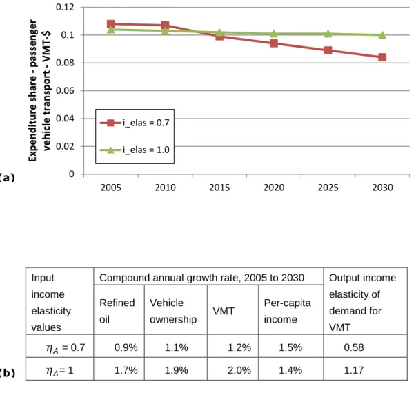
The income elasticity of demand for passenger vehicle transport can be updated over time by calculating a new subsistence level, which is then used in the solution of the model (although initial model runs assume that the income elasticity of demand is constant and less than or equal to 1). Although some discrepancy will always exist between the specified (used to calculate the subsistence expenditure) and the observed (calculation based on model outputs), the discrepancy is the result of price effects and substitution within the model. The input elasticities are defined based on empirical estimates that attempt to separate the effect of income on demand for vehicle services from price and other effects, while output elasticities reflect the combined influence of income and price effects over time. The effect of changing the input income elasticity of demand for - in the United States from 1 to 0.70 is shown in Figure 4. The expenditure share of passenger vehicle transport declines even when the income elasticity is equal to 1 because of substitution allowed between services supplied by purchased transport and passenger vehicle transport. Modest increases in fuel prices over the same period increase the relative price of vehicle transport services, inducing a weak shift to other modes.14
14 A description of the data sources used to calibrate income elasticities of demand in the 16 EPPA model regions, the full derivation of relevant equations, and an analysis of sensitivities to income elasticity of demand assumptions are described in the Supplementary Material.
Figure 4. The effect of changing the specified income elasticity of demand in the United States in the MIT EPPA model from 1 to 0.70 in the reference (No Policy) case on (a) expenditures share for passenger vehicle transport and (b) growth rates for VMT, vehicles, refined oil demand, and per capita income through 2030.
Input income elasticity values
Compound annual growth rate, 2005 to 2030 Output income elasticity of demand for VMT Refined oil Vehicle ownership VMT Per-capita income = 0.7 0.9% 1.1% 1.2% 1.5% 0.58 = 1 1.7% 1.9% 2.0% 1.4% 1.17 0 0.02 0.04 0.06 0.08 0.1 0.12 2005 2010 2015 2020 2025 2030 Expe nd itur e sha re - pa ss en ger veh ic le tr an spo rt - VMT -$ i_elas = 0.7 i_elas = 1.0 (a) (b)
3.2 Development 2: Modeling Opportunities for Vehicle Efficiency Improvement
Investment in vehicle fuel efficiency provides one option for reducing fuel use and associated expenditures in response to an increase in fuel prices. This investment can take the form of improvements to existing ICE-only vehicles, or the adoption of alternative fuel vehicles (AFVs, discussed in Section 3.3). Often vehicle efficiency improvements are modeled using exogenous engineering projections to specify a rate of efficiency improvement over time, without
considering the role of fuel prices or any trade-offs in vehicle attributes required to achieve efficiency improvements. For instance, vehicle downsizing decreases vehicle size and weight, attributes that the consumer may value and may be unwilling to forego in favor of fuel savings. Moreover, policies that set different vehicle fuel economy targets or that result in fuel price increases are likely to affect investment in existing vehicle fuel economy and in alternative fuel vehicles (AFVs). Model developments implemented here aim to capture endogenously the underlying relationships among policy, fuel prices, and consumer investment in fuel economy.
The extent at which fuel efficiency improvements translate into direct reductions in fuel use depends primarily on two factors—the rate of fleet turnover (the net of sale of new vehicles and scrappage of old vehicles, which is limited to a fraction of the total fleet each year), and the willingness of manufacturers to produce—and consumers to invest—in more fuel efficient vehicles as fuel prices rise. A new structure of the passenger vehicle transport sector was introduced to simulate both of these constraints on raising the average efficiency of the vehicle fleet. Here I consider only incremental improvements to existing vehicles. Development 3 (Section 3.3) involves introducing alternatives to today’s gasoline-powered ICE.
3.2.1 Opportunities for Vehicle Efficiency Improvements: New Sector Structure To model the technological opportunities for improving vehicle efficiency in a manner consistent with engineering and related cost (bottom-up) data, a new structure was introduced into the passenger vehicle transport sector. The guiding intuition for the new structure was the need to model the fuel and base vehicle as complementary goods, while allowing for investment in fuel efficiency in response to changes in fuel price.
A schematic representation of the split between VMT from new and used vehicles is shown in the utility function in the second level (blue box) shown in Figure 1. The new sector structure for new (zero to five) year old vehicles is shown in the third level (green box) in Figure 1. The structure of the used vehicle sector is the same, but with a fixed (Leontief) structure to reflect the fact that efficiency characteristics have been determined in earlier periods. The main departure from past approaches is to separate the powertrain efficiency cost component from a base vehicle capital cost component. Initially, we assume that the base vehicle capital cost component (which captures a range of energy-neutral vehicle attributes) of driving one mile remains constant and represents the capital expenditure on an average vehicle absent the powertrain, while the powertrain capital cost component trades off with fuel expenditures as determined by an elasticity of substitution between fuel and powertrain capital ( ). Both the vehicle
to cover interest and depreciation associated with the purchase of a more fuel efficient vehicle. In the model, these inputs are drawn from the “other” industries classification, which includes automotive manufacturing in the underlying GTAP database. The cost associated with incremental increases in vehicle efficiency is captured by the powertrain capital input. The balance of powertrain capital cost and fuel cost reflects the relative mix of energy-saving and energy-intensive technology implemented in the average U.S. vehicle in the initial model calibration year, 2004. The substitution elasticity between fuel and vehicle capital determines how investment in vehicle efficiency responds to fuel price changes. Parameterization of this key elasticity will be discussed later in this section.
3.2.2 Modeling Fleet Turnover Using a Two-vintage Approach
The approach to fleet turnover taken here is essentially to model the miles-traveled by vehicles divided into two vintages: a “new” vehicle vintage (0-5 year old vehicles) and a “used” vehicle vintage (over 5 years old). The used vehicle fleet is in turn characterized by four sub-vintages, which have unique average efficiencies and reflect the differential contributions to VMT. Older vehicles tend to be less efficient (especially if regulations force new vehicle efficiency to improve), and are also driven less. The two-vintage structure has several
advantages: 1) it allows detailed vehicle efficiency, driving, and fleet turnover data to be used in regions where available, 2) it provides a simple representation of stock turnover that can be parameterized with minimal data in regions where data is not available, and 3) it is consistent with the EPPA structure, which uses five-year time steps.
The rate of vehicle stock turnover limits how fast new technology can be adopted into the in-use vehicle fleet. Even the most inexpensive, off-the-shelf technologies will be limited by the rate of fleet turnover since they are mostly applied in new vehicles sold (as opposed to being used to retrofit existing vehicles). The differentiation of vehicle services according to age (vintage) introduces a first constraint on the rate of adoption of new technologies. A new
technology can only be applied to 0 to 5 year old vehicles that provide the new vehicle transport services.
The preservation of efficiency characteristics in vehicles as they age is an important function of the vintaging structure. In each period the efficiency characteristics assumed for the new vehicles are passed to the first vintage of the used fleet, the first used vintage to the second, and so forth. The fifth (oldest) vintage (vehicles 20 years old or more) from the previous period is scrapped. In a CGE model efficiency characteristics are captured in the underlying cost shares, which are handed off from one vintage to the next (see Paltsev et al., 2005 for more detail on capital vintaging in the MIT EPPA model). In the model only the values of capital services provided by the new and used vehicle fleet are represented explicitly. The shares for the used fleet represent the average of the shares for the surviving vintages, weighted by the share of miles they contribute to total used VMT according to Equation 7:
(
) ∑ (
)
(7)
In this equation are the expenditures shares for each input to a used vehicle vintage V in period . The coefficients in front of each term on the right-hand side of the equation represent the mileage shares of each vintage in the used fleet, where corresponds to the vehicle-miles driven by each of the four used vintages in period , and corresponds to total miles driven by the used vehicle fleet.
Representing the contributions of new and used vehicles to passenger vehicle transport has several advantages over previous approaches. First, it constrains the rate at which new
technology can be adopted in the vehicle fleet, adding realism to projections. Second, it allows for the simulation of vintage-differentiated policies (e.g. policies that bear on technology choices in the new vehicle fleet only, such as the Corporate Average Fuel Economy (CAFE) standard in the United States). Third, it can provide insight into the impact of policies on fleet turnover, for example, if consumers respond by substituting between usage of new and used vehicles, which may differ in terms of their efficiency.
3.2.3 Fuel Efficiency Response to Fuel Price in New Passenger Vehicles
Advanced vehicle technology will predominantly affect fuel use and GHG emissions through its installation in new vehicles. Econometric studies have documented that consumer demand for fuel efficiency in new vehicles responds to fuel prices (Klier & Linn, 2008). In a macroeconomic model it is important to capture how policy signals induce consumers and manufacturers to respond by increasing vehicle fuel efficiency at different levels of policy stringency.
The modeler faces a decision about how to parameterize the elasticity of substitution between fuel and vehicle powertrain capital. Passenger vehicle transport is essentially a production function for VMT that enters on the utility side of representative agent’s economic activities. A perfectly rational economic agent will respond to rising fuel costs by investing in efficiency improvements according to the cost-effectiveness of technologies, starting with the solution that offers reductions at the lowest marginal cost of abatement. This willingness to substitute capital to reduce fuel consumption is captured by the elasticity of substitution, in Figure 5.
To estimate the approach adopted here stems from a method previously used in CGE models to parameterize substitution elasticities using bottom-up data. In this case I construct a marginal abatement cost curve for vehicle fuel use reduction, following previous work (Hyman
et al., 2002). By identifying the piece cost (or direct manufacturing cost, before retail margins
are included) of various abatement technologies and the associated reduction in fuel consumption (on the vehicle level), it is possible to gain a sense of the order in which these technologies would be adopted in different vehicle segments. Together with appropriate assumptions about maximum adoption rates in various size and weight classes that comprise the passenger vehicle fleet, it is possible to order the potential contribution of individual technologies to total reduction in gasoline use at the fleet level according to cost per gallon of gasoline displaced. The
of each technology must be specified at a particular point in time. A marginal abatement cost curve thus reflects a static picture of fuel or GHG emissions reductions that could be achieved at a given marginal cost, in this case for the benchmark year 2004.
Using the procedure described in Hyman et al. (2002), it is possible to derive a relationship between the price elasticity of demand for fuel required per mile and the elasticity of substitution between fuel and vehicle powertrain capital, according to Equation 8:
(8)
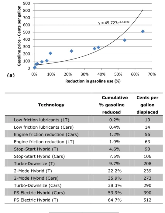
As before is the expenditure share for the primary good of interest—in this case, the per-mile fuel requirement. The elasticity of demand for fuel can be found by fitting an exponential function to the empirically-derived ordering of reductions according to cost. The composite curve for all passenger vehicles is shown in Figure 5. The fitted parameters are related to the elasticity of supply of GHG emissions abatement. Given that total output of the fuel-powertrain capital nest is fixed by the Leontief (zero) substitution assumption in the upper nest in the structure (intuitively, a base vehicle will start from some fixed combination of fuel and fuel abatement), the elasticity of supply of abatement technology is identically equal to the elasticity of demand for fuel.15 Using Equation 8 and the value of the expenditure share on fuel in the fuel-powertrain capital bundle, it is straightforward to obtain , the elasticity of substitution.
Care was taken when constructing the MAC curve to ensure that mutually exclusive technology trajectories were not included. For example, the MAC curve for today’s ICE-only vehicles is intended to capture incremental changes to the internal combustion engine that include hybridization, turbo-charging and engine downsizing (TCD), as well as dieselization. However since TCD and dieselization represent a mutually exclusive technology trajectories (while, by contrast, hybridization and TCD could be complementary), only the most
cost-effective path was included (in this case, hybridization and TCD). A similar procedure is applied to estimate the MAC curve for light-trucks as well as for alternative powertrains. Differences in the cost-effectiveness of the technology across vehicle market segments were considered in the estimation of total fuel reduction potential.
y = 45.727e4.4492x 0 100 200 300 400 500 600 700 800 900 0% 10% 20% 30% 40% 50% 60% 70% Gaso lin e p ri ce Ce n ts p e r gal lo n
Reduction in gasoline use (%)
Figure 5. Marginal abatement cost curves for passenger vehicles in 2011, with (a) marginal cost of reducing fuel use through application of technology graphed against
cumulative fuel use reduction, (b) the table of cost-effectiveness values from EPA (2010) used to parameterize the curve, and (c) estimated values of the substitution elasticity and related variables for each curve.
Technology Cumulative % gasoline reduced Cents per gallon displaced
Low friction lubricants (LT) 0.2% 10
Low friction lubricants (Cars) 0.4% 14
Engine friction reduction (Cars) 1.2% 56
Engine friction reduction (LT) 1.9% 63
Stop-Start Hybrid (T) 4.6% 90
Stop-Start Hybrid (Cars) 7.5% 106
Turbo-Downsize (T) 9.7% 208
2-Mode Hybrid (T) 22.2% 239
2-Mode Hybrid (Cars) 35.9% 273
Turbo-Downsize (Cars) 38.3% 290
PS Electric Hybrid (Cars) 53.9% 390
PS Electric Hybrid (T) 64.7% 512 Variable Estimate 0.73 -0.225 4.449 0.70 (a) (b) (c)
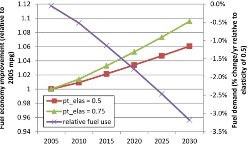
An initial range of estimates for obtained from the calibration exercise was 0.5 to 0.76.16 By implementing these two alternative parameter values in the EPPA model, total fleet fuel economy and the discrepancy in fuel use over time were simulated in the absence of policy as shown in Figure 6.
Figure 6. Simulated improvement in the vehicle fleet fuel economy (both new and used vehicles) and total fuel use using alternative elasticities of substitution between fuel and powertrain capital ( = 0.5, 0.75) in the MIT EPPA model in a reference (no policy) scenario.
The parameterization of shares and the elasticity of substitution assume that the production and adoption of more efficient vehicles will respond to fuel cost given a particular consumer discount rate. In the MIT EPPA model, the discount rate used is 4 percent; other models may assume slightly higher or lower rates. As such it reflects the decision of a rational manufacturer responding to a rational consumer—i.e. each is indifferent between $1 of expenditures today and $1 of future discounted expenditures. Our analysis initially proceeds based on the lower
discounting assumption (4%). However the new model structure allows this assumption to be relaxed in order to simulate higher discount rates, which have been observed in the econometrics literature (Hausman, 1979; Allcott & Wozny, 2010).
3.3 Development 3: Representation of Alternative Fuel Vehicles
Alternative fuel vehicles (vehicles that run on fuels other than conventional petroleum-based fuels, such as gasoline and diesel) have been advocated as a breakthrough that will enable reductions in fuel use beyond those attainable with incremental improvements to ICE-only
16 For more discussion see Supplementary Material.
-3.5% -3.0% -2.5% -2.0% -1.5% -1.0% -0.5% 0.0% 0.94 0.96 0.98 1 1.02 1.04 1.06 1.08 1.1 1.12 2005 2010 2015 2020 2025 2030 Fu e l d e m an d (% c h an ge /y r re lativ e to e lasti ci ty o f 0.5 ) Fu e l e co n o m y im p ro ve m e n t (r e lativ e to 20 05 m p g) pt_elas = 0.5 pt_elas = 0.75 relative fuel use
vehicle technology. These vehicles are often the target of public policy initiatives aimed at achieving reductions in both petroleum consumption and GHG emissions. These vehicles include electric and plug-in hybrid electric vehicles (EVs and PHEVs), compressed natural gas vehicles (CNGVs), and hydrogen fuel cell electric vehicles (FCEVs). These vehicles currently cost more to purchase than an ICE-only vehicle of comparable size and performance, but could offer fuel savings relative to ICE-only vehicles, depending on gasoline prices, which lead to a wide range of current estimates and forecasts of total ownership costs. Below I describe how AFVs are represented in the EPPA model.
Recent developments in vehicle technology and related policy suggest that some fraction of future VMT may come from alternative fuel vehicles over the next 40 years, particularly if changing conditions (including relative prices of fuels and the availability of infrastructure) make these technologies attractive to consumers. The degree of adoption may in turn be influenced by policy design. The cost and abatement potential offered by alternative fuel vehicles is
represented in the model as follows.
3.3.1 Parameterization and Key Elasticities
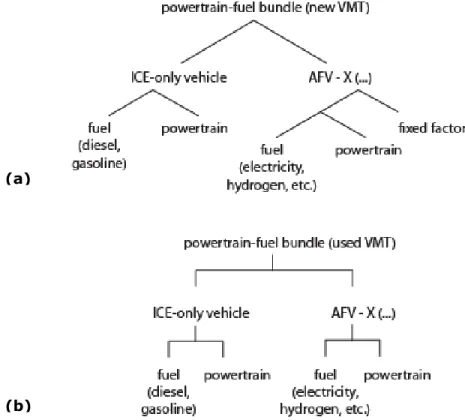
In previous CGE models that include a disaggregated transport sector, AFVs have been represented as a separate sector that competed with internal combustion engine (ICE-only) vehicles in the provision of passenger vehicle transport services (see for example Karplus et al., 2010). Each AFV variant (PHEV, EV) was described by a vehicle capital, services, and fuel shares, plus a markup assigned to the vehicle share to capture the incremental cost of the alternative propulsion system. Our new approach (see Figure 1, green box at the bottom of the consumption nest) is to contain all of the powertrain options within a single household vehicle transport services nest (the left side of each diagram in Figure 7), and to have alternative powertrains compete as perfect substitutes at the level of the fuel-vehicle capital nest. The base vehicle and services inputs (on the right-hand side of the nest in Figure 1) are assumed to remain constant across powertrain types. This procedure reduces the number of cost shares that must be estimated for each powertrain type. It is based on the assumption that the primary distinguishing feature of alternative fuel vehicles is the powertrain, and that the incremental cost reflects the contribution of the powertrain and its impact on the fuel requirement as it compares to other powertrain-fuel combinations.
So far, plug-in hybrid electric vehicles (PHEVs) and electric vehicles (EVs) are represented as backstop technologies to the ICE-only vehicle. A backstop technology is a potential alternative to an in-use technology that is not cost competitive in the benchmark year but may be adopted in future model periods as a result of changing relative input costs or policy conditions. A
description of the previous method for implementing plug-in hybrid electric vehicles as a backstop technology can be found in Karplus et al. (2010). Although this analysis is focused on electric-drive vehicles, other vehicle types, such as the CNGV or FCEV could be easily added to this structure for specific studies.
Figure 7. The inclusion of alternative powertrain types (denoted by AFV–X, where X could be a PHEV, EV, CNGV, and/or FCEV) in the (a) new and (b) used passenger vehicle transport sectors in the MIT EPPA model.
The criteria for including an advanced vehicle type as a separate powertrain (as opposed to capturing any fuel reduction potential through the elasticity of substitution between fuel and abatement capital) is whether the technology requires a fuel not mixable with conventional formulations of gasoline or diesel. Modifications to the internal combustion engine, including the addition of a turbo-charger, engine downsizing, or transmission improvements do not represent fundamentally new vehicle technology platforms and are thus represented as opportunities for reducing the fuel use of the internal combustion engine as described in Section 3.2 above. However, plug-in hybrid electric vehicles and electric-only vehicles require grid-supplied electricity and are thus represented separately. The calculation of cost shares based on the levelized cost of ownership is discussed in detail in Karplus (2011).
As in the case of the ICE vehicle, for each of the alternative fuel vehicle types, fuel
consumption can be reduced with increased capital expense. To parameterize the values of these elasticities, we follow a method similar to our approach for the ICE and estimate a marginal abatement cost curve that starts by assuming the existing fuel efficiency and emissions
characteristics for each backstop technology and models the fuel reduction in percentage terms.
(b) (a)
3.3.2 Constraints on Adoption
Several hurdles must be overcome before an advanced vehicle technology can gain a significant share of the new vehicle market and contribute to emissions reductions. The new modeling approach captures separately the effect of three constraints on the development and deployment of AFVs. First, fleet turnover (described in Section 3.2) allows advanced
technologies to only enter through the new vehicle fleet, while the used vehicle fleet transforms only gradually over time. Second, we capture how the incremental cost of the advanced
technology relative to the existing technology changes over time by parametrically varying an exogenous assumption about the rate of cost reduction. Third, we represent fixed costs associated with scaling up production of advanced technologies and obtaining acceptance in a
heterogeneous consumer market. Since fleet turnover has been described previously, this section focuses on the modeling of the second and third constraints.
Reduction in the incremental vehicle capital cost on a precompetitive technology could occur as a result of ongoing technological progress (possibly through a substantial R&D effort aimed at a particularly promising technology). The goal is to capture the intuition that a technology
expected to have large market potential will attract R&D funds even before it becomes cost competitive, and these R&D investments will have the effect of bringing the technology closer to cost parity. Here I represent cost reductions through a constant absolute reduction in the markup of 1% in each model period, although more complex, and potentially endogenous,
representations of cost reductions over time could be easily implemented.
Finally, once a vehicle technology reaches cost parity with the incumbent, we still expect its market adoption to be constrained by a variety of factors on both the supply and demand sides of the market. Incorporating new vehicle technology into production-ready models can take
multiple years, and cannot be implemented across all new vehicle segments simultaneously without requiring additional resources. Production capacity must be allocated and scaled up in response to rising demand. Consumers may hesitate to adopt a particular vehicle technology if specialized refueling infrastructure is required but not readily available. Moreover, only a subset of consumers will be willing to buy and have driving needs well suited to take advantage of particular alternative fuel vehicle types. To capture these additional barriers to adoption, we parameterize a small share of the new powertrain production structure to include an additional fixed cost associated with AFV adoption, denoted fixed factor in Figure 7 (Karplus et al., 2010). Although these costs are often not directly observed, the value of this fixed cost requirement is parameterized based on evidence of the adoption rates for vehicle powertrain technology, including dieselization in Europe and the global adoption of off-grid hybrid vehicles.
4. SENSITIVITY EXERCISES USING NEW MODEL DEVELOPMENTS
In order to illustrate the advantages of the new model structure, I briefly describe the
sensitivity to alternative assumptions related to each of the model developments described above for the case of the United States. It is important to note that relative to the unchanged model, the projected fuel use and GHG emissions from passenger vehicles is significantly lower (data not
shown). This difference is expected because the new model structure reflects expected saturation of transportation expenditures in the household budget (and thus VMT and related spending increases less rapidly than income). The new model structure also represents more realistically the investment in vehicle efficiency as fuel prices rise, offsetting the increase in gasoline demand and GHG emissions. A more detailed report of these outputs is provided in Karplus (2011). Below I demonstrate the impact of varying both the relationship between income and demand for vehicle travel (Development 1), the responsiveness of vehicle efficiency to fuel price
(Development 2), and the impact of the availability of the PHEV (Development 3) by showing the impact of these relationships under “best” and “worst” case assumptions. The assumptions are shown below in Table 2. The cost of the PHEV is assumed to be 25% higher relative to the ICE-only vehicle.
Table 2. List of key sensitivities used to define the best and worst case scenarios.
Parameter Income elasticity† Substitution elasticity (+/- 25%) PHEV available?
Best case 0.65 0.94 Yes
Worst case 0.75 0.56 No
Reference case 0.70 0.75 No
†Value shown is initial value through 2020, which then decreases by 0.01 every 5 years thereafter. The values were based on alternative trajectories for household vehicle ownership and are shown in Karplus (2011).
The outcomes of the sensitivity analysis are shown in Table 3 below. When VMT grows less rapidly with income, efficiency improvements are inexpensive, and a PHEV option is available, cumulative fuel use is reduce around 9% relative to reference. By contrast, in the worst case scenario, cumulative fuel use increases around 7% relative to reference. The relative magnitude of the increase is smaller than the decrease in the best case scenario because with high demand there is more price pressure to invest in efficiency improvements, even though they are relatively expensive due to the low elasticity ( ) and the fact that the PHEV is not available. For the range of values examined here, it is interesting to note that even in the best case scenario, fuel use and GHG emissions in 2050 remain far from the levels scientists and policymakers claim are needed to reach energy and climate policy goals (U.S. CCSP, 2007).
Table 3. Sensitivity of cumulative fuel use, total fossil CO2 emissions, and consumption
change in the United States to “best” and “worst” case assumptions.
Quantities of Interest Best Worst Reference
Fuel use (billion gal) -9.26% 7.27% 7,023
Total fossil CO2 emissions (mmt CO2) -1.68% 1.35% 367,966
5. SUMMARY AND EXTENSIONS
This article has described a technology-rich approach to modeling passenger vehicle transport in a CGE model. This three-part approach could be applied, with some modifications, to model demand for any energy-intensive consumer durable product in a CGE framework.17 Broadly, the three parts of this model development reflect three important generic considerations: 1) the relationship between total expenditures, expenditures on durable services, and the usage of the durable in physical units (miles-traveled for vehicles, load-hours for washing machines, or heating degree days for air conditioners), 2) representing capital stock turnover and vintage-differentiated opportunities for efficiency improvement, and 3) the availability and cost of substitute technologies with substantially different fuel requirements. Augmenting the model structure to facilitate a detailed engineering-based representation of the underlying physical system requires extensive and reliable data for calibration.
The new developments provide a platform that can be adapted depending on the purposes of the analysis. For instance, additional vehicle powertrain and fuel options could be easily added by expanding the number of technological substitutes on the left side of the vehicle transport services nest. Other modifications could be undertaken as needed to address specific questions.
Acknowledgments
This project was supported by the BP-MIT Advanced Conversion Research Project and the MIT Joint Program on the Science and Policy of Global Change. The Integrated Global System Model (IGSM) and its economic component, the MIT Emissions Predictions and Policy Analysis (EPPA) model, used in this analysis is supported by a consortium of government, industry, and foundation sponsors of the MIT Joint Program on the Science and Policy of Global Change. (For a complete list of sponsors, see: http://globalchange.mit.edu).
3. REFERENCES
Abeles, E.C., 2004: Analysis of Light-Duty Vehicle Price Trends in the U.S.: How Vehicle Prices Changed Relative to Consumers, Compliance Costs and a Baseline Measure for 1975 - 2001. Davis, CA: Institute of Transportation Studies, University of California, Davis.
Allcott, H. and N. Wozny, 2010: Gasoline Prices, Fuel Economy, and the Energy Paradox. Cambridge, MA: Center for Economic and Environmental Policy Research.
(http://web.mit.edu/ceepr/www/publications/workingpapers/2010-003.pdf ).
An, F. and J. DeCicco, 2007: Trends in Technical Efficiency Trade-offs for the U.S. Light Vehicle Fleet. SAE Technical Paper Series 2007-01-1325. Detroit, MI: SAE International. Arndt, C., Robinson, S. and F. Tarp, 2001: Parameter estimation for a computable general
equilibrium model: A maximum entropy approach. Economic Modeling, 19(3), 375-398.
17
The approach described here for passenger vehicle transport can be readily adapted to models that disaggregate demand for transport services within the consumption function. With some additional effort passenger vehicle transport could be disaggregated from household consumption in most CGE models as needed (for more discussion see Paltsev et al., 2004).