The ChainQueen differentiable physics engine

The ChainQueen Differentiable Physics Engine

by

Yuanming Hu

Submitted to the Department of Electrical Engineering and Computer

Science

in partial fulfillment of the requirements for the degree of

Master of Science in Computer Science and Engineering

at the

MASSACHUSETTS INSTITUTE OF TECHNOLOGY

February 2019

c

○ Massachusetts Institute of Technology 2019. All rights reserved.

Author . . . .

Department of Electrical Engineering and Computer Science

November 16, 2018

Certified by . . . .

Wojciech Matusik

Associate Professor of Electrical Engineering and Computer Science

Thesis Supervisor

Accepted by . . . .

Leslie A. Kolodziejski

Professor of Electrical Engineering and Computer Science

Chair, Department Committee on Graduate Students

The ChainQueen Differentiable Physics Engine

by

Yuanming Hu

Submitted to the Department of Electrical Engineering and Computer Science on November 16, 2018, in partial fulfillment of the

requirements for the degree of

Master of Science in Computer Science and Engineering

Abstract

Physical simulators have been widely used in robot planning and control. Among them, differentiable simulators are particularly favored, as they can be incorporated into gradient-based optimization algorithms that are efficient in solving inverse problems such as optimal control and motion planning. Simulating deformable objects is, however, more challenging compared to rigid body dynamics. The underlying physical laws of deformable objects are more complex, and the resulting systems have orders of magnitude more degrees of freedom and therefore they are significantly more computationally expensive to simulate. Computing gradients with respect to physical design or controller parameters is typically even more computationally challenging. In this paper, we propose a real-time, differentiable hybrid Lagrangian-Eulerian physical simulator for deformable objects, ChainQueen, based on the Moving Least Squares Material Point Method (MLS-MPM). MLS-MPM can simulate deformable objects including contact and can be seamlessly incorporated into inference, control and co-design systems. We demonstrate that our simulator achieves high precision in both forward simulation and backward gradient computation. We have successfully employed it in a diverse set of control tasks for soft robots, including problems with nearly 3, 000 decision variables.

Thesis Supervisor: Wojciech Matusik

Acknowledgments

First of all, I am grateful to my thesis advisor Prof. Wojciech Matusik, without whom this work would not have been made possible. His insightful guidance, generous support and kind encouragements have not only greatly accelerated the development of this project, but also cultivated my ability to conduct high-quality research.

Then, I would like to thank my collaborators. I feel privileged to have the opportunity to work with Prof. Bo Zhu, Prof. Eftychios Sifakis, Prof. Chenfanfu Jiang, Prof. William T. Freeman, Prof. Joshua B. Tenenbaum and Prof. Daniela Rus during my master study. Also, I am fortunate to collaborate with Jiancheng Liu, Andrew Spielberg, Tao Du, Jiajun Wu, Liang Shi, Haixiang Liu, Hao He, Yu Fang, Ziheng Ge, Ziyin Qu, Yixin Zhu, Dr. Andre Pradhana, who have been both excellent colleagues and supportive friends of mine.

Finally and most importantly, I would thank my family and my girlfriend. I am indebted to them, since I have spent very limited time together with them in the past year, due to the physical distance across the oceans.

This thesis is dedicated to everyone above, and many others who have supported me.

Contents

1 Introduction 13

2 Related Work 15

2.1 Material Point Method . . . 15 2.2 Differentiable Simulation and Control . . . 16

3 Background: The Moving Least Squares Material Point Method 17

4 The Differentiable Moving Least Squares Material Point Method 21

5 Evaluation 25

5.1 Efficiency . . . 25 5.2 Accuracy . . . 26

6 Applications 29

6.1 Physical Parameter Inference . . . 29 6.2 Control . . . 29 6.3 Co-design . . . 31

7 Discussion 35

A Differentiation 37

A.1 Variable dependencies . . . 37 A.2 Backward Particle to Grid (P2G) . . . 41 A.3 Backward Grid Operations . . . 42

A.4 Backward Grid to Particle (G2P) . . . 42 A.5 Friction Projection Gradients . . . 45

List of Figures

3-1 One time step of MLS-MPM. Top arrows are for forward simulation and bottom ones are for back propagation. A controller is embedded in the P2G process to generate actuation given particle configurations. . 19

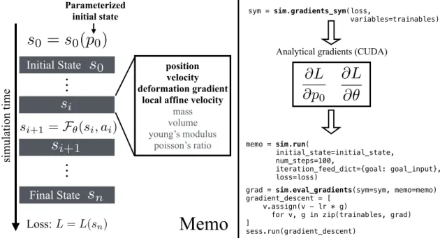
4-1 Left: A “memo" object consists all information of a single simulation execution, including all the time step state information (position, veloc-ity, deformation gradients etc.), and parameters for the initial state 𝑝0,

policy parameter 𝜃. Right: Code samples to get the symbolic differenti-ation (top) and memo, evaluate gradients out of the memo and symbolic differentiation, and finally use them for gradient descent (bottom). . . 24

5-1 Experiments on the pneumatic leg. Row (A, B) Footage and simulator results of a bouncing experiment with the leg dropping at 15 cm. Row (C, D) Actuation test. . . 28

6-1 System Identification. The initial density 1 for elastic ball A leads to limited momentum to push ball B to its destination C. After several gradient descent iterations, the inferenced (optimized) density 2.26 gives the right amount of momentum for ball B to stop at C at the end of the simulation. . . 30 6-2 A soft 2D walker with controller optimized using gradient descent,

aiming to achieve a maximum distance after 600 simulation steps. The walker has four actuators (left, marked by letter ‘A’s) with each capable of stretching or compressing in the vertical direction. . . 31

6-3 3D robots with optimized controllers: quadruped runner, robotic finger, and crawler. The crawler is optimized with an open-loop controller, taking only trigonometric phase functions of time 𝑡 as inputs. . . 33 6-4 Final poses of the arm swing task. Lighter colors refer to stiffer

regions. (c) Final pose of the fixed-stiffness 300% initial Young’s modulus arm. (d) Final pose of the fixed-stiffness 300% initial Young’s modulus arm. (e) Final pose of the co-optimized arm. Actuation cost is 95.5% that of the fixed 100% initial Young’s modulus arm and converges. Only the co-optimized arm is able to fully reach its target. The final optimized spatially varying stiffness of the arm has lower stiffness on the outside of the bend, and higher stiffness inside, promoting more bend to the left. Qualitatively, this is similar in effect to the pleating on soft robot fingers. . . 34 6-5 Convergence of the arm reaching task for co-design vs. fixed arm designs.

The fixed designs can make progress but not complete the task, while with co-design, the task can be completed and the actuation cost is lower. Constraint violation is the norm of two constraints: distance of end-effector to goal and mean squared velocity of the particles. . . 34

List of Tables

3.1 List of notations for MLS-MPM. . . 18 5.1 Performance comparisons on a NVIDIA GTX 1080 Ti GPU. F stands

for forward simulation and B stands for backward differentiation. TF indicates the TensorFlow implementation. When benchmarking our simulator with CUDA we use the C++ instead of python interface to avoid the extra overhead due to the TensorFlow runtime library. . . . 26 5.2 Relative error in simulation and gradient precision. Empty values are

because of too short time for collision to happen. . . 27 A.1 List of notations for MLS-MPM. . . 38

Chapter 1

Introduction

Robot planning and control algorithms often rely on physical simulators for prediction and optimization [32, 6]. In particular, differentiable physical simulators enable the use of gradient-based optimizers, significantly improving control efficiency and precision. Motivated by this, there has been extensive research on differentiable rigid body simulators, using approximate [2, 24] and exact [5, 31, 8] methods.

Significant challenges remain for deformable objects. First, simulating the motion of deformable objects is slow, because they have much higher degrees of freedom (DoFs). Second, contact detection and resolution is challenging for deformable objects, due to their changing geometries and potential self-collisions. Third, closed-form and efficient computation of gradients is challenging in the presence of contact. As a consequence, current simulation methods for soft objects cannot be effectively used for solving inverse problems such as optimal control and motion planning.

In this work, we introduce a real-time, differentiable physical simulator for de-formable objects, building upon the Moving Least Squares Material Point Method (MLS-MPM) [16]. We name our simulator ChainQueen*. The Material Point Method (MPM) is a hybrid Lagrangian-Eulerian method that uses both particles and grid nodes for simulation [29]. MLS-MPM accelerates and simplifies traditional MPM using a moving least squares force discretization. In ChainQueen, we introduce the first fully differentiable MLS-MPM simulator with respect to both state and model

parameters, with both forward simulation and back-propagation running efficiently on GPUs. We demonstrate the ability to efficiently calculate gradients with respect to the entire simulation. This enables many novel applications for soft robotics in-cluding optimization-based closed-loop controller design, trajectory optimization, and co-design of robot geometry, materials, and control.

As a particle-grid-based hybrid simulator, MPM simulates objects of various states, such as liquid (e.g., water), granular materials (e.g., sand), and elastoplastic materials (e.g., snow and human tissue). ChainQueen focuses on elastic materials for soft robotics. It is fully differentiable and 4_{− 9× faster than the current state of the} art. Numerical and experimental validation suggest that ChainQueen achieves high precision in both forward simulation and backward gradient computation.

ChainQueen’s differentiability allows it to support gradient-based optimization for control and system identification. By performing gradient descent on controller parameters, our simulator is capable of solving these inverse problems on a diverse set of complex tasks, such as optimizing a 3D soft walker controller given an objective. Similarly, gradient descent on physical design parameters, enables inference of physical properties (e.g. mass, density and Young’s modulus) of objects and optimizing design for a desired task.

In addition to benchmarking ChainQueen’s performance and demonstrating its capabilities on a diverse set of inverse problems, we have interfaced our simulator with high-level python scripts to make ChainQueen user-friendly. Users at all levels will be able to develop their own soft robotics systems using our simulator, without the need to understand its low-level details. We will open-source our code and data and we hope they can benefit the robotics community.

Chapter 2

Related Work

2.1

Material Point Method

The material point method has been extensively developed from both a solid mechan-ics [29] and computer graphmechan-ics [19] perspective. As a hybrid Eulerian-Langrangian method, MPM has demonstrated its versatility in simulating snow [28, 12], sand [21, 3], non-Newtonion fluids [25], cloth [18, 13], solid-fluid coupling [9, 30], rigid body cou-pling, and cutting [16]. [10] also proposed an adaptive MPM scheme to concentrate computation resources in the regions of interest.

There are many benefits of using MPM for soft robotics. First, MPM is a well-founded and physically-accurate discretization method and can be derived through the weak form of conservation laws. Such a physically based approach makes it easier to match simulation with real-world experiments. Second, MPM is friendly to parallelization on modern hardware architectures. Closely related to our work is a high-performance GPU implementation [11] by Gao et al., from which we borrow many useful optimization practices. Though efficient when solving forward simulation, their simulator is not differentiable, making it inefficient for inverse problems in robotics and learning. Third, MPM naturally handles large deformation and (self-)collision, which are common in soft robotics, but often not modeled in, e.g., mesh-based approaches due to computational expense. Finally, the continuum dynamics (including soft object collision) are governed by the smooth (and differentiable) potential energy, making

the whole system differentiable.

Our simulator, ChainQueen, is fully differentiable and the first simulator that applies MPM to soft robotics.

2.2

Differentiable Simulation and Control

Recently, there has been an increasing interest in building differentiable simulators for planning and control. For rigid bodies, [1], [2] and [24] proposed to approximate object interaction with neural nets; later, [26] explored their usage in control. Approximate analytic differentiable rigid body simulators have also been proposed [5, 4]. Such systems have been deployed for manipulation and planning [33].

Differentiable simulators for deformable objects have been less studied. Recently, [27] proposed SPNets for differentiable simulation of position-based fluids [22]. The particle interactions are coded as neural network operations and differentiability is achieved via automatic differentiation in PyTorch. A hierarchical particle-based object representation using neural networks is also proposed in [24]. Instead of approximating physics using neural networks, ChainQueen differentiates MLS-MPM, a well physically founded discretization scheme derived from continuum mechanics. In summary, our simulator can be used for a more diverse set of objects; it is more physically plausible, and runs faster.

Chapter 3

Background: The Moving Least

Squares Material Point Method

In this chapter, we provide some background on the material point method (MPM), which is used for forward simulation.

We use the moving least squares material point method (MLS-MPM) [16] to discretize continuum mechanics, which is governed by the following two equations:

𝜌𝐷v

𝐷𝑡 =∇ · 𝜎 + 𝜌g (momentum conservation), (3.1) 𝐷𝜌

𝐷𝑡 + 𝜌∇ · v = 0 (mass conservation). (3.2) MLS-MPM is a simpler and more efficient variant of classical MPM. The simplicity of MLS-MPM has greatly reduced the work needed to differentiate it. Here we briefly cover the basics of MLS-MPM and readers are referred to [19] and [16] for a comprehensive introduction of MPM and MLS-MPM, respectively.

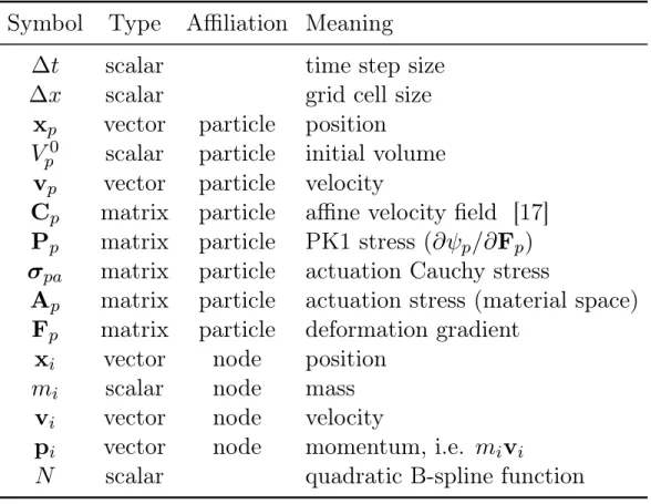
The material point method is a hybrid Eulerian-Lagrangian method, where both particles and grid nodes are used. Simulation state information is transferred back-and-forth between these two representations. We summarize the notations we use in this paper in Table 3.1. Subscripts are used to denote particle (𝑝) and grid nodes (𝑖), while superscripts (𝑛, 𝑛 + 1) are used to distinguish quantities in different time steps.

Table 3.1: List of notations for MLS-MPM. Symbol Type Affiliation Meaning

∆𝑡 scalar time step size ∆𝑥 scalar grid cell size

x𝑝 vector particle position

𝑉0

𝑝 scalar particle initial volume

v𝑝 vector particle velocity

C𝑝 matrix particle affine velocity field [17]

P𝑝 matrix particle PK1 stress (𝜕𝜓𝑝/𝜕F𝑝)

𝜎𝑝𝑎 matrix particle actuation Cauchy stress

A𝑝 matrix particle actuation stress (material space)

F𝑝 matrix particle deformation gradient

x𝑖 vector node position

𝑚𝑖 scalar node mass

v𝑖 vector node velocity

p𝑖 vector node momentum, i.e. 𝑚𝑖v𝑖

𝑁 scalar quadratic B-spline function

1. Particle-to-grid transfer (P2G). Particles transfer mass 𝑚𝑝, momentum

(𝑚v)𝑛

𝑝, and stress-contributed impulse to their neighbouring grid nodes, using

the Affine Particle-in-Cell method (APIC) [17] and moving least squares force discretization [16], weighted by a compact B-spline kernel 𝑁 :

𝑚𝑛_𝑖 = ∑︁ 𝑝 𝑁 (x𝑖− x𝑛𝑝)𝑚𝑝, (3.3) G𝑛_𝑝 = ₋ 4 ∆𝑥2∆𝑡𝑉 0 𝑝P 𝑛 𝑝F 𝑛𝑇 𝑝 + 𝑚𝑝C𝑛𝑝, (3.4) p𝑛_𝑖 = ∑︁ 𝑝 𝑁 (x𝑖− x𝑛𝑝)[︀𝑚𝑝v𝑛𝑝 + G 𝑛 𝑝(x𝑖− x𝑛𝑝)]︀ . (3.5)

P2G Grid op. G2P G2P gradients (backward P2G) Grid op. gradients … … P2G gradients (backward G2P)

particle states at tn grid momentum grid velocity particle states at tn+1

Figure 3-1: One time step of MLS-MPM. Top arrows are for forward simulation and bottom ones are for back propagation. A controller is embedded in the P2G process to generate actuation given particle configurations.

conditions and gravity for simplicity. Boundary conditions are usually applied as a projection on grid node velocity.

3. Grid-to-particle transfer (G2P). Particles gather updated velocity v𝑛+1 𝑝 ,

local velocity field gradients C𝑛+1_𝑝 and position x𝑛+1_𝑝 form neighbouring grid nodes. At the same time, the constitutive model properties (for example, deformation gradients F𝑛+1_𝑝 ) are updated. MLS-MPM unifies the local velocity gradient computation and affine velocity field computation, leading to higher efficiency and simplicity.

v_𝑝𝑛+1 = ∑︁ 𝑖 𝑁 (x𝑖− x𝑛𝑝)v 𝑛 𝑖, (3.7) C𝑛+1_𝑝 = 4 ∆𝑥2 ∑︁ 𝑖 𝑁 (x𝑖− x𝑛𝑝)v 𝑛 𝑖(x𝑖− x𝑛𝑝) 𝑇 , (3.8) F𝑛+1_𝑝 = (I + ∆𝑡C𝑛+1_𝑝 )F𝑛_𝑝, (3.9) x𝑛+1_𝑝 = x𝑛_𝑝 + ∆𝑡v𝑛+1_𝑝 . (3.10)

For soft robotics, we additionally introduce an actuation model. Inspired by actuators such as [14], we designed an actuation model that expands or stretches particle 𝑝 via an additional Cauchy stress A𝑝 = F𝑝𝜎𝑝𝑎F𝑇𝑝, with 𝜎𝑝𝑎= Diag(𝑎𝑥, 𝑎𝑦, 𝑎𝑧)

– the stress in the material space. This framework supports the use of other actuation models including pneumatic, hydraulic, and cable-driven actuators. Fig. 3-1 illustrates

Chapter 4

The Differentiable Moving Least

Squares Material Point Method

MLS-MPM is naturally differentiable. Although the forward MPM simulation has been extensively used in computer graphics, the backward direction (differentiation or back-propagation) is largely unexplored. The backward gradients can be derived given forward simulation relationships. Here we show the gradients of x𝑛_𝑝 based on

forward simulation, as an example: x𝑛+1_𝑝 = x𝑛_𝑝+ Δ𝑡v𝑛+1𝑝 (4.1) v𝑛+1_𝑝 = ∑︁ 𝑖 𝑁 (x𝑖− x𝑛𝑝)v𝑛𝑖 (4.2) C𝑛+1_𝑝 = 4 Δ𝑥2 ∑︁ 𝑖 𝑁 (x𝑖− x𝑛𝑝)v𝑛𝑖(x𝑖− x𝑛𝑝)𝑇 (4.3) p𝑛_𝑖 = ∑︁ 𝑝 𝑁 (x𝑖− x𝑛𝑝) [︂ 𝑚𝑝v𝑛𝑝 + (︂ −_Δ𝑥42Δ𝑡𝑉 0 𝑝P𝑛𝑝F𝑛𝑇𝑝 + 𝑚𝑝C𝑛𝑝 )︂ (x𝑖− x𝑛𝑝) ]︂ (4.4) 𝑚𝑛 𝑖 = ∑︁ 𝑝 𝑁 (x𝑖− x𝑛𝑝)𝑚𝑝 (4.5) G𝑝 := (︂ −_Δ𝑥42𝑉 0 𝑝Δ𝑡P𝑛𝑝F𝑛𝑇𝑝 + 𝑚𝑝C𝑛𝑝 )︂ (4.6) =_⇒ (4.7) 𝜕𝐿 𝜕x𝑛 𝑝𝛼 = [︃ 𝜕𝐿 𝜕x𝑛+1𝑝 𝜕x𝑛+1 𝑝 𝜕x𝑛 𝑝 + 𝜕𝐿 𝜕v𝑛+1𝑝 𝜕v𝑛+1 𝑝 𝜕x𝑛 𝑝 + 𝜕𝐿 𝜕C𝑛+1𝑝 𝜕C𝑛+1 𝑝 𝜕x𝑛 𝑝 + 𝜕𝐿 𝜕p𝑛 𝑖 𝜕p𝑛 𝑖 𝜕x𝑛 𝑝 + 𝜕𝐿 𝜕𝑚𝑛 𝑖 𝜕𝑚𝑛 𝑖 𝜕x𝑛 𝑝 ]︃ 𝛼 (4.8) = 𝜕𝐿 𝜕x𝑛+1𝑝𝛼 (4.9) +∑︁ 𝑖 ∑︁ 𝛽 𝜕𝐿 𝜕v𝑛+1_𝑝𝛽 𝜕𝑁 (x𝑖− x𝑛𝑝) 𝜕x𝑖𝛼 v𝑛_𝑖𝛽 (4.10) +∑︁ 𝑖 ∑︁ 𝛽 (4.11) 4 Δ𝑥2 {︃ − 𝜕𝐿 𝜕C𝑛+1_𝑝𝛽𝛼𝑁 (x𝑖− x 𝑛 𝑝)v𝑖𝛽+ ∑︁ 𝛾 𝜕𝐿 𝜕C𝑛+1_𝑝𝛽𝛾 𝜕𝑁 (x𝑖− x𝑛𝑝) 𝜕x𝑖𝛼 v𝑖𝛽(x𝑖𝛾− x𝑝𝛾) }︃ (4.12) +∑︁ 𝑖 ∑︁ 𝛽 (4.13) 𝜕𝐿 𝜕p𝑛 𝑖𝛽 [︂_{𝜕𝑁 (x} 𝑖− x𝑛𝑝) 𝜕x𝑖𝛼 (︀𝑚𝑝v𝑛𝑝𝛽+ [G𝑝(x𝑖− x𝑛𝑝)]𝛽)︀ − 𝑁(x𝑖− x𝑛𝑝)G𝑝𝛽𝛼 ]︂ (4.14) +𝑚𝑝 ∑︁ 𝑖 𝜕𝐿 𝜕𝑚𝑛 𝑖 𝜕𝑁 (x𝑖− x𝑛𝑝) 𝜕x𝑖𝛼 (4.15)

We refer the readers to Appendix A for more details on gradient derivation. Based on the gradients we have derived analytically, we have designed a high-performance

respect to the initial state, as well as to the controller parameters that are used in each state. We cache all the simulation states in memory, using a “memo” object. Though the underlying differentiation is complicated, we have designed a simple high-level TensorFlow interface on which end-users can build their applications (Fig. 4-1).

Our high-performance implementation* takes advantage of the computational power of modern GPUs through CUDA. We also implemented a reference implementation in TensorFlow. Note that programming physical simulation as a “computation graph” using high-level frameworks such as TensorFlow is less inefficient. In fact, when all the overheads are gone, our optimized CUDA solver is 132_{× faster than the TensorFlow} reference version. This is because TensorFlow is optimized towards deep learning applications where data granularity is much larger and memory access pattern is much more regular than physical simulation, and limited CPU-GPU bandwidth. In contrast, our CUDA implementation is tailored for MLS-MPM and explicitly optimized for parallelism and locality, thus delivering high-performance.

position velocity deformation gradient

local affine velocity

mass volume young’s modulus poisson’s ratio

s

= s

(p

)

si

s

…

…

s

s

@L

@p

Memo

grad = sim.eval_gradients(sym=sym, memo=memo) gradient_descent = [

v.assign(v - lr * g)

for v, g in zip(trainables, grad) ] sess.run(gradient_descent)

@L

@✓

s

=

F

(s

, a

)

Analytical gradients (CUDA)

Figure 4-1: Left: A “memo" object consists all information of a single simulation execution, including all the time step state information (position, velocity, deformation gradients etc.), and parameters for the initial state 𝑝0, policy parameter 𝜃. Right:

Code samples to get the symbolic differentiation (top) and memo, evaluate gradients out of the memo and symbolic differentiation, and finally use them for gradient descent (bottom).

Chapter 5

Evaluation

In this section, we conduct a comprehensive study of the efficiency and accuracy of our system, in both 2D and 3D.

5.1

Efficiency

Instead of using complex geometries, a simple falling cube is used for performance benchmarking, to ensure easy analysis and reproducibility. We benchmark the perfor-mance of our CUDA simulator against NVIDIA Flex [23], a popular PBD physical simulator capable of simulating deformable objects. Note that both PBD and MLS-MPM needs substepping iterations to ensure high stiffness. To ensure fair comparison, we set a Young’s modulus, Poisson’s ration and density so that visually ChainQueen gives similar results to Flex. We used two steps per frame and four iterations per step in Flex. Note that setting exactly the same parameters is not possible since in PBD there is no explicitly defined physical quantity such as Young’s modulus.

We summarize the quantitative performance in Table 5.1. Our CUDA simulator provides higher speed than Flex, when the number of particles are the same. It is also worth noting that the TensorFlow implementation is much slower, due to excessive runtime overheads.

Table 5.1: Performance comparisons on a NVIDIA GTX 1080 Ti GPU. F stands for forward simulation and B stands for backward differentiation. TF indicates the TensorFlow implementation. When benchmarking our simulator with CUDA we use the C++ instead of python interface to avoid the extra overhead due to the TensorFlow runtime library.

Approach Impl. # Particles Time per Frame Flex (3D) CUDA 8,024 3.5 ms (286 FPS) Ours (3D, F) CUDA 8,000 0.392 ms (2,551 FPS) Ours (3D, B) CUDA 8,000 0.406 ms (2,463 FPS) Flex (3D) CUDA 61,238 6 ms (167 FPS) Ours (3D, F) CUDA 64,000 1.594 ms (628 FPS) Ours (3D, B) CUDA 64,000 1.774 ms (563 FPS) Ours (3D, F) CUDA 512,000 10.501 ms (92 FPS) Ours (3D, B) CUDA 512,000 11.594 ms (86 FPS) Ours (2D, F) TF 6,400 13.2 ms (76 FPS) Ours (2D, B) TF 6,400 35.7 ms (28 FPS) Ours (2D, F) CUDA 6,400 0.10 ms (10,000 FPS) Ours (2D, B) CUDA 6,400 0.14 ms (7,162 FPS)

5.2

Accuracy

We design five test cases to evaluate the accuracy of both forward simulation and backward gradient evaluation:

1. A1 (analytic, 3D, float32 precision): final position w.r.t. initial velocity (with collision). This case tests conservation of momentum, gradient accuracy and stability of back-propagation.

2. A2 (analytic, 3D, float32 precision): same as A1 but with one collision to a friction-less wall.

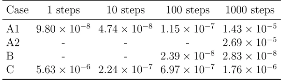
Table 5.2: Relative error in simulation and gradient precision. Empty values are because of too short time for collision to happen.

Case 1 steps 10 steps 100 steps 1000 steps A1 9.80_{× 10}−8 4.74_{× 10}−8 1.15_{× 10}−7 1.43_{× 10}−5

A2 - - - 2.69_{× 10}−5

B - - 2.39_{× 10}−8 2.83_{× 10}−8

C 5.63_{× 10}−6 2.24_{× 10}−7 6.97_{× 10}−7 1.76_{× 10}−6

simulation process.

5. D1 (experimental, pneumatic actuator, actuation) In order to evaluate our simulator’s real-world accuracy, we compared the deformation of a physical actuator to a virtual one. The physical actuator has four pneumatic chambers which can be inflated with an external pump, arranged in a cross-shape. Inflating the individual chambers bends the actuator away from that chamber. The actuator was cast using Smooth-On Dragon Skin 30.

6. D2 (experimental, pneumatic actuator, bouncing) In a second test, we dropped the same actuator from a 15 cm height, and compared its dynamic motion to a simulation.

In 3D analytic test cases, where gradients w.r.t. initial velocity can be directly evaluated as in Table 5.2. For the experimental comparisons, the results are shown in Fig. 5-1. In addition to our simulator’s high performance and accuracy, it is worth noting that that the gradients remain stable in the long term, within up to 1000 time steps.

Chapter 6

Applications

The most attractive feature of our simulator is the existence of quickly computable gradients, which allows the use of much more efficient gradient-based optimization algorithms. In this section, we show the effectiveness of our differentiable simulator on gradient-based optimization tasks, including physical inference, control for soft robotics, and co-design of robotic arms.

6.1

Physical Parameter Inference

ChainQueen can be used to infer physical system properties given its observed motion, e.g. perform gradient descent to infer the relative densities of two colliding elastic balls (see Figure 6-1, ball A moving to the right hitting ball B, and ball B arrives the destination C). Gradient-based optimization infers that relative density of ball A is 2.26, which constitutes to the correct momentum to push B to C. Such capability makes it useful for real-world robotic tasks such as system identification.

6.2

Control

We can optimize regression-based controllers for soft robots and efficiently discover stable gaits. The controller takes as input the state vector z, which includes target position, the center of mass position, and velocity of each composed soft component.

Figure 6-1: System Identification. The initial density 1 for elastic ball A leads to limited momentum to push ball B to its destination C. After several gradient descent

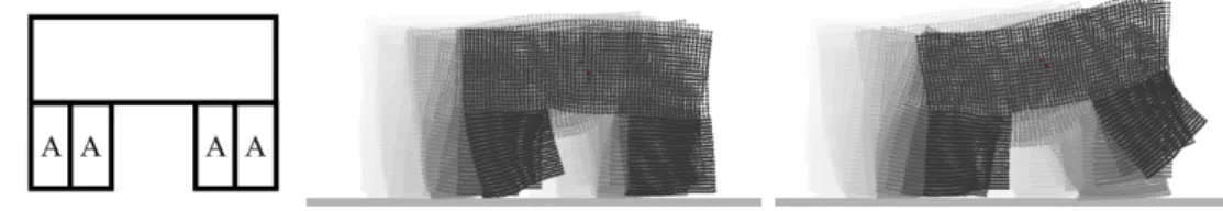
Figure 6-2: A soft 2D walker with controller optimized using gradient descent, aiming to achieve a maximum distance after 600 simulation steps. The walker has four actuators (left, marked by letter ‘A’s) with each capable of stretching or compressing in the vertical direction.

In our examples, the actuation vector a for up to 16 actuators is generated by the controller in each time step. During optimization, we perform gradient descent on variables W and b, where a = tanh (Wz + b) is the actuation-generating controller. We have designed a series of experiments (Fig. 6-2 and Fig. 6-3). Gradient-based optimizers successfully compute desired closed loop controllers controllers within only tens or hundreds of iterations.

6.3

Co-design

Our simulator is capable of not only providing gradients with respect to dynamics and controller parameters, but also with respect to structural design parameters, enabling co-design of soft robots. To demonstrate this, we designed a multi-link robot arm (two links, two joints each with two side-by-side actuators; all parts deformable). Similar to shooting method trajectory optimization, actuation for each time step is solved for, along with the time-invariant Young’s modulus of the system for each particle. In our task, we optimized the end-effector of the arm to reach a goal ball with final 0 arm velocity, and minimized for actuation cost∑︀𝑁

𝑖=0𝑢𝑇𝑖 𝑢𝑖𝑑𝑡, where 𝑢𝑖 is the actuation

vector at timestep 𝑖, and 𝑁 is the total number of timesteps. This is a dynamic task and the target pose cannot be reached in a static equilibrium. NLOPT’s sequential least squares programming algorithm was used for optimization [20]. We compared our co-design solution to fixed designs. The designed stiffness distribution is shown in Fig. 6-4, along with controls. The convergence for the different tasks can be seen in Fig. 6-5. As can be seen, only the co-design arm fully converges to the target goal, and with lower actuation cost. Actuation for each chamber was clamped, and rnges

of 30% to 400% of a dimensionless initial Young’s modulus were allowed and chosen large enough such as to require a swing instead of a simple bend.

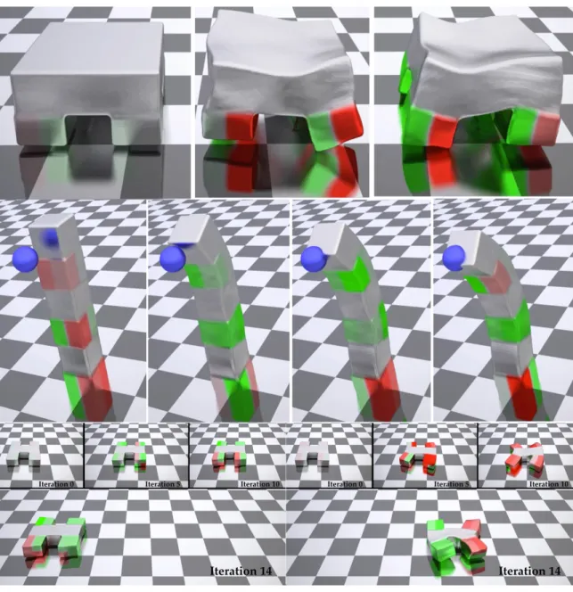
Figure 6-3: 3D robots with optimized controllers: quadruped runner, robotic finger, and crawler. The crawler is optimized with an open-loop controller, taking only trigonometric phase functions of time 𝑡 as inputs.

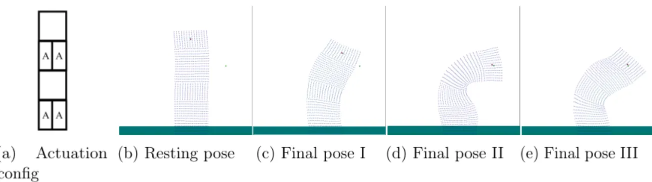
(a) Actuation config

(b) Resting pose (c) Final pose I (d) Final pose II (e) Final pose III

Figure 6-4: Final poses of the arm swing task. Lighter colors refer to stiffer regions. (c) Final pose of the fixed-stiffness 300% initial Young’s modulus arm. (d) Final pose of the fixed-stiffness 300% initial Young’s modulus arm. (e) Final pose of the co-optimized arm. Actuation cost is 95.5% that of the fixed 100% initial Young’s modulus arm and converges. Only the co-optimized arm is able to fully reach its target. The final optimized spatially varying stiffness of the arm has lower stiffness on the outside of the bend, and higher stiffness inside, promoting more bend to the left. Qualitatively, this is similar in effect to the pleating on soft robot fingers.

0

5

10

15

20

25

30

35

40

45

10

10

10

10

Constraint Violation

Fixed 300% Initial Young's

Fixed 100% Initial Young's

Co-design

Chapter 7

Discussion

We have presented ChainQueen, a differentiable simulator for soft robotics, and demonstrated how it can be deployed for inference, control, and co-design. ChainQueen has the potential to accelerate the development of soft robots. We have also developed a high-performance GPU implementation for ChainQueen, which we will open source.

One interesting future direction is to couple our soft object simulation with rigid body simulation, as done in [16]. As derived in [7], the ∆𝑡 limit for explicit time integration is 𝐶∆𝑥√︀_𝐸𝜌, where 𝐶 is a constant close to one, 𝜌 is the density, and 𝐸 is the Young’s modulus. That means for very stiff materials (e.g., rigid bodies), only a very restrictive ∆𝑡 can be used. However, a rigid body simulator should probably be employed in the realm of nearly-rigid objects and coupled with our deformable body simulator. Combining our simulator with existing rigid-body simulators using Compatible Particle-in-Cell [16] can be an interesting direction.

Appendix A

Differentiation

In this appendix, we discuss the detailed steps for backward gradient computation in ChainQueen, i.e. the differentiable Moving Least Squares Material Point Method (MLS-MPM) [16]. Again, we summarize the notations in Table A.1. We assume fixed particle mass 𝑚𝑝, volume 𝑉𝑝0, hyperelastic constitutive model (with potential energy

𝜓𝑝 or Young’s modulus 𝐸𝑝 and Poisson’s ratio 𝜈𝑝) for simplicity.

A.1

Variable dependencies

Table A.1: List of notations for MLS-MPM.

Symbol

Type

Affiliation Meaning

Δ𝑡

scalar

time step size

Δ𝑥

scalar

grid cell size

x

vector

particle

position

𝑉

scalar

particle

initial volume

v

vector

particle

velocity

C

matrix

particle

affine velocity field [17]

P

matrix

particle

PK1 stress (𝜕𝜓

/𝜕F

)

𝜎

matrix

particle

actuation Cauchy stress

A

matrix

particle

actuation stress (material space)

F

matrix

particle

deformation gradient

x

vector

node

position

𝑚

scalar

node

mass

v

vector

node

velocity

p

vector

node

momentum, i.e.

𝑚

v

𝑁

scalar

quadratic B-spline function

P𝑛_𝑝 = P𝑛_𝑝(F𝑛_𝑝) + F𝑝𝜎𝑝𝑎𝑛 (A.1) 𝑚𝑛_𝑖 = ∑︁ 𝑝 𝑁 (x𝑖− x𝑛𝑝)𝑚𝑝 (A.2) p𝑛_𝑖 = ∑︁ 𝑝 𝑁 (x𝑖− x𝑛𝑝) [︂ 𝑚𝑝v𝑛𝑝 + (︂ − 4 Δ𝑥2Δ𝑡𝑉 0 𝑝P𝑛𝑝F𝑛𝑇𝑝 + 𝑚𝑝C𝑛𝑝 )︂ (x𝑖− x𝑛𝑝) ]︂ (A.3) v𝑛_𝑖 = 1 𝑚𝑛 𝑖 p𝑛_𝑖 (A.4) v𝑛+1_𝑝 = ∑︁ 𝑖 𝑁 (x𝑖− x𝑛𝑝)v𝑛𝑖 (A.5)

The forward variable dependency is as follows: x𝑛+1_{𝑝 ← x}𝑛_𝑝, v𝑛+1_𝑝 (A.9) v𝑛+1_{𝑝 ← x}𝑛_𝑝, v𝑛_𝑖 (A.10) C𝑛+1_{𝑝 ← x}𝑛_𝑝, v𝑛_𝑖 (A.11) F𝑛+1_{𝑝 ← F}𝑛_𝑝, C𝑛+1_𝑝 (A.12) p𝑛_{𝑖 ← x}𝑛_𝑝, C𝑛_𝑝, v𝑛_𝑝, P𝑛_𝑝, F𝑛_𝑝 (A.13) v𝑛_{𝑖 ← p}𝑛_𝑖, 𝑚𝑛_𝑖 (A.14) P𝑛_{𝑝 ← F}𝑛_𝑝, 𝜎𝑛_𝑝𝑎 (A.15) 𝑚𝑛_{𝑖 ← x}𝑛_𝑝 (A.16)

During back-propagation, we have the following reversed variable dependency:

x𝑛+1_𝑝 , v_𝑝𝑛+1, C𝑛+1_𝑝 , p𝑛+1_𝑖 , 𝑚𝑖 ← x𝑛𝑝 (A.17) p𝑛_{𝑖 ← v}𝑛_𝑝 (A.18) x𝑛+1_{𝑝 ← v}𝑛+1_𝑝 (A.19) v_𝑝𝑛+1, C𝑛+1_{𝑝 ← v}𝑛_𝑖 (A.20) F𝑛+1_𝑝 , P𝑛_𝑝, p𝑛_{𝑖 ← F}𝑛_𝑝 (A.21) F𝑛+1_{𝑝 ← C}𝑛+1_𝑝 (A.22) p𝑛_{𝑖 ← C}𝑛_𝑝 (A.23) v𝑛_{𝑖 ← p}𝑛_𝑖 (A.24) v𝑛_{𝑖 ← 𝑚}𝑛_𝑖 (A.25) p𝑛_{𝑖 ← P}𝑛_𝑝 (A.26) P𝑛_{𝑝 ← 𝜎}𝑛_𝑝𝑎 (A.27)

x𝑛_{𝑝 → x}𝑛+1_𝑝 , v_𝑝𝑛+1, C𝑛+1_𝑝 , p𝑛+1_𝑖 , 𝑚𝑖 (A.28) v𝑛_{𝑝 → p}𝑛_𝑖 (A.29) v𝑛+1_{𝑝 → x}𝑛+1_𝑝 (A.30) v𝑛_{𝑖 → v}𝑛+1_𝑝 , C𝑛+1_𝑝 (A.31) F𝑛_{𝑝 → F}𝑛+1_𝑝 , P𝑛_𝑝, p𝑛_𝑖 (A.32) C𝑛+1_{𝑝 → F}𝑛+1_𝑝 (A.33) C𝑛_{𝑝 → p}𝑛_𝑖 (A.34) p𝑛_{𝑖 → v}𝑛_𝑖 (A.35) 𝑚𝑛_{𝑖 → v}𝑛_𝑖 (A.36) P𝑛_{𝑝 → p}𝑛_𝑖 (A.37) 𝜎𝑛_{𝑝𝑎 → P}𝑛_𝑝 (A.38)

In the following sections, we derive detailed gradient relationships, in the order of actual gradient computation. The frictional boundary condition gradients are postponed to the end since it is less central, though during computation it belongs to grid operations. Back-propagation in ChainQueen is essentially a reversed process of forward simulation. The computation has three steps, backward particle to grid (P2G), backward grid operations, and backward grid to particle (G2P).

A.2

Backward Particle to Grid (P2G)

(A, P2G) For v𝑛+1_𝑝 , we have

x𝑛+1_𝑝 = x𝑛_𝑝 + ∆𝑡v𝑛+1_𝑝 (A.39) =_⇒ 𝜕𝐿 𝜕v𝑛+1 𝑝𝛼 = [︂ 𝜕𝐿 𝜕x𝑛+1 𝑝 𝜕x𝑛+1 𝑝 𝜕v𝑛+1 𝑝 ]︂ 𝛼 (A.40) = ∆𝑡 𝜕𝐿 𝜕x𝑛+1 𝑝𝛼 . (A.41) (B, P2G) For C𝑛+1 𝑝 , we have F𝑛+1_𝑝 = (I + ∆𝑡C𝑛+1_𝑝 )F𝑛_𝑝 (A.42) =_⇒ 𝜕𝐿 𝜕C𝑛+1_𝑝𝛼𝛽 = [︂ 𝜕𝐿 𝜕F𝑛+1 𝑝 𝜕F𝑛+1_𝑝 𝜕C𝑛+1 𝑝 ]︂ 𝛼𝛽 (A.43) = ∆𝑡∑︁ 𝛾 𝜕𝐿 𝜕F𝑛+1 𝑝𝛼𝛾 F𝑛_𝑝𝛽𝛾. (A.44)

Note, the above two gradients should also include the contributions of _𝜕v𝜕𝐿𝑛 𝑝 and

𝜕𝐿 𝜕C𝑛

𝑝 respectively, with 𝑛 being the next time step.

(C, P2G) For v𝑛 𝑖, we have v𝑛+1_𝑝 = ∑︁ 𝑖 𝑁 (x𝑖− x𝑛𝑝)v𝑛𝑖 (A.45) C𝑛+1_𝑝 = 4 Δ𝑥2 ∑︁ 𝑖 𝑁 (x𝑖− x𝑛𝑝)v𝑛𝑖(x𝑖− x𝑛𝑝)𝑇 (A.46) =⇒ _𝜕v𝜕𝐿𝑛 𝑖𝛼 = [︃ ∑︁ 𝑝 𝜕𝐿 𝜕v𝑝𝑛+1 𝜕v𝑛+1 𝑝 𝜕v𝑛 𝑖 +∑︁ 𝑝 𝜕𝐿 𝜕C𝑛+1𝑝 𝜕C𝑛+1 𝑝 𝜕v𝑛 𝑖 ]︃ 𝛼 (A.47) = ∑︁ 𝑝 ⎡ ⎣ 𝜕𝐿 𝜕v𝑛+1𝑝𝛼 𝑁 (x𝑖− x𝑛𝑝) + 4 Δ𝑥2𝑁 (x𝑖− x 𝑛 𝑝) ∑︁ 𝛽 𝜕𝐿 𝜕C𝑛+1_𝑝𝛼𝛽(x𝑖𝛽− x𝑝𝛽) ⎤ ⎦. (A.48)

A.3

Backward Grid Operations

(D, grid) For p𝑛_𝑖, we have

v𝑛_𝑖 = 1 𝑚𝑛 𝑖 p𝑛_𝑖 (A.49) =_⇒ 𝜕𝐿 𝜕p𝑛 𝑖𝛼 = [︂ 𝜕𝐿 𝜕v𝑛 𝑖 𝜕v_𝑖𝑛 𝜕p𝑛 𝑖 ]︂ 𝛼 (A.50) = 𝜕𝐿 𝜕v𝑛 𝑖𝛼 1 𝑚𝑛 𝑖 . (A.51)

(E, grid) For 𝑚𝑛

𝑖, we have v𝑛_𝑖 = 1 𝑚𝑛 𝑖 p𝑛_𝑖 (A.52) =_⇒ 𝜕𝐿 𝜕𝑚𝑛 𝑖 = 𝜕𝐿 𝜕v𝑛 𝑖 𝜕v𝑛 𝑖 𝜕𝑚𝑛 𝑖 (A.53) = ₋ 1 (𝑚𝑛 𝑖)2 ∑︁ 𝛼 p𝑛_𝑖𝛼 𝜕𝐿 𝜕v𝑛 𝑖𝛼 (A.54) = ₋ 1 𝑚𝑛 𝑖 ∑︁ 𝛼 v𝑛_𝑖𝛼 𝜕𝐿 𝜕v𝑛 𝑖𝛼 . (A.55)

(G, G2P) For P𝑛_𝑝, we have p𝑛_𝑖 = ∑︁ 𝑝 𝑁 (x𝑖− x𝑛𝑝) [︂ 𝑚𝑝v𝑛𝑝 + (︂ −_Δ𝑥42Δ𝑡𝑉 0 𝑝P𝑛𝑝F𝑛𝑇𝑝 + 𝑚𝑝C𝑛𝑝 )︂ (x𝑖− x𝑛𝑝) ]︂ (A.59) =_⇒ 𝜕𝐿 𝜕P𝑛 𝑝𝛼𝛽 = [︂ 𝜕𝐿 𝜕p𝑛 𝑖 𝜕p𝑛 𝑖 𝜕P𝑛 𝑝 ]︂ 𝛼𝛽 (A.60) = −∑︁ 𝑖 𝑁 (x𝑖− x𝑛𝑝) 4 Δ𝑥2Δ𝑡𝑉 0 𝑝 ∑︁ 𝛾 𝜕𝐿 𝜕p𝑛 𝑖𝛼 F𝑛_𝑝 𝛾𝛽(x𝑖𝛾− x 𝑛 𝑝𝛾). (A.61) (H, G2P) For F𝑛 𝑝, we have F𝑛+1_𝑝 = (I + Δ𝑡C𝑛+1𝑝 )F𝑛𝑝 (A.62) P𝑛_𝑝 = P𝑛𝑝(F𝑛𝑝) + F𝑝𝜎𝑛𝑝𝑎 (A.63) p𝑛_𝑖 = ∑︁ 𝑝 𝑁 (x𝑖− x𝑛𝑝) [︂ 𝑚𝑝v𝑝𝑛+ (︂ −_Δ𝑥42Δ𝑡𝑉 0 𝑝P𝑛𝑝F𝑛𝑇𝑝 + 𝑚𝑝C𝑛𝑝 )︂ (x𝑖− x𝑛𝑝) ]︂ (A.64) =_⇒ 𝜕𝐿 𝜕F𝑛 𝑝𝛼𝛽 = [︃ 𝜕𝐿 𝜕F𝑛+1𝑝 𝜕F𝑛+1 𝑝 𝜕F𝑛 𝑝 + 𝜕𝐿 𝜕P𝑛 𝑝 𝜕P𝑛 𝑝 𝜕F𝑛 𝑝 + 𝜕𝐿 𝜕p𝑛 𝑖 𝜕p𝑛 𝑖 𝜕F𝑛 𝑝 ]︃ 𝛼𝛽 (A.65) = ∑︁ 𝛾 𝜕𝐿 𝜕F𝑛+1_𝑝𝛾𝛽 (I𝛾𝛼+ Δ𝑡C 𝑛+1 𝑝𝛾𝛼) + ∑︁ 𝛾 ∑︁ 𝜂 𝜕𝐿 𝜕P𝑝𝛾𝜂 𝜕2_Ψ 𝑝 𝜕F𝑛 𝑝𝛾𝜂𝜕F𝑛𝑝𝛼𝛽 (A.66) + ∑︁ 𝛾 𝜕𝐿 𝜕P𝑛 𝑝𝛼𝛾 𝜎𝑝𝑎𝛽𝛾 (A.67) +∑︁ 𝑖 −𝑁(x𝑖− x𝑛𝑝) ∑︁ 𝛾 𝜕𝐿 𝜕p𝑛 𝑖𝛾 4 Δ𝑥2Δ𝑡𝑉 0 𝑝P𝑛𝑝𝛾𝛽(x𝑖𝛼− x𝑛𝑝𝛼). (A.68)

(I, G2P) For C𝑛_𝑝, we have

p𝑛_𝑖 = ∑︁ 𝑝 𝑁 (x𝑖− x𝑛𝑝) [︂ 𝑚𝑝v𝑛𝑝 + (︂ −_Δ𝑥42Δ𝑡𝑉 0 𝑝P𝑛𝑝F𝑛𝑇𝑝 + 𝑚𝑝C𝑛𝑝 )︂ (x𝑖− x𝑛𝑝) ]︂ (A.69) =_⇒ 𝜕𝐿 𝜕C𝑛 𝑝𝛼𝛽 = [︃ ∑︁ 𝑖 𝜕𝐿 𝜕p𝑛 𝑖 𝜕p𝑛 𝑖 𝜕C𝑛 𝑝 ]︃ 𝛼𝛽 (A.70) = ∑︁ 𝑖 𝑁 (x𝑖− x𝑛𝑝) 𝜕𝐿 𝜕p𝑛 𝑖𝛼 𝑚𝑝(x𝑖𝛽− x𝑛𝑝𝛽). (A.71)

(J, G2P) For x𝑛_𝑝, we have x𝑛+1_𝑝 = x𝑛_𝑝+ Δ𝑡v𝑛+1𝑝 (A.72) v𝑛+1_𝑝 = ∑︁ 𝑖 𝑁 (x𝑖− x𝑛𝑝)v𝑛𝑖 (A.73) C𝑛+1_𝑝 = 4 Δ𝑥2 ∑︁ 𝑖 𝑁 (x𝑖− x𝑛𝑝)v𝑛𝑖(x𝑖− x𝑛𝑝)𝑇 (A.74) p𝑛_𝑖 = ∑︁ 𝑝 𝑁 (x𝑖− x𝑛𝑝) [︂ 𝑚𝑝v𝑛𝑝 + (︂ −_Δ𝑥42Δ𝑡𝑉 0 𝑝P𝑛𝑝F𝑛𝑇𝑝 + 𝑚𝑝C𝑛𝑝 )︂ (x𝑖− x𝑛𝑝) ]︂ (A.75) 𝑚𝑛 𝑖 = ∑︁ 𝑝 𝑁 (x𝑖− x𝑛𝑝)𝑚𝑝 (A.76) G𝑝 := (︂ −_Δ𝑥42𝑉 0 𝑝Δ𝑡P𝑛𝑝F𝑛𝑇𝑝 + 𝑚𝑝C𝑛𝑝 )︂ (A.77) =_⇒ (A.78) 𝜕𝐿 𝜕x𝑛 𝑝𝛼 = [︃ 𝜕𝐿 𝜕x𝑛+1𝑝 𝜕x𝑛+1 𝑝 𝜕x𝑛 𝑝 + 𝜕𝐿 𝜕v𝑛+1𝑝 𝜕v𝑛+1 𝑝 𝜕x𝑛 𝑝 + 𝜕𝐿 𝜕C𝑛+1𝑝 𝜕C𝑛+1 𝑝 𝜕x𝑛 𝑝 + 𝜕𝐿 𝜕p𝑛 𝑖 𝜕p𝑛 𝑖 𝜕x𝑛 𝑝 + 𝜕𝐿 𝜕𝑚𝑛 𝑖 𝜕𝑚𝑛 𝑖 𝜕x𝑛 𝑝 ]︃ 𝛼 (A.79) = 𝜕𝐿 𝜕x𝑛+1𝑝𝛼 (A.80) +∑︁ 𝑖 ∑︁ 𝛽 𝜕𝐿 𝜕v𝑛+1_𝑝𝛽 𝜕𝑁 (x𝑖− x𝑛𝑝) 𝜕x𝑖𝛼 v𝑛_𝑖𝛽 (A.81) +∑︁ 𝑖 ∑︁ 𝛽 (A.82) 4 Δ𝑥2 {︃ − 𝜕𝐿 𝜕C𝑛+1_𝑝𝛽𝛼𝑁 (x𝑖− x 𝑛 𝑝)v𝑖𝛽+ ∑︁ 𝛾 𝜕𝐿 𝜕C𝑛+1_𝑝𝛽𝛾 𝜕𝑁 (x𝑖− x𝑛𝑝) 𝜕x𝑖𝛼 v𝑖𝛽(x𝑖𝛾− x𝑝𝛾) }︃ (A.83) +∑︁ 𝑖 ∑︁ 𝛽 (A.84) 𝜕𝐿 𝜕p𝑛 𝑖𝛽 [︂_{𝜕𝑁 (x} 𝑖− x𝑛𝑝) 𝜕x𝑖𝛼 (︀𝑚𝑝v𝑛𝑝𝛽+ [G𝑝(x𝑖− x𝑛𝑝)]𝛽)︀ − 𝑁(x𝑖− x𝑛𝑝)G𝑝𝛽𝛼 ]︂ (A.85) +𝑚𝑝 ∑︁ 𝑖 𝜕𝐿 𝜕𝑚𝑛 𝑖 𝜕𝑁 (x𝑖− x𝑛𝑝) 𝜕x𝑖𝛼 (A.86) (K, G2P) For 𝜎𝑛 𝑝𝑎, we have P𝑛 = P𝑛(F𝑛) + F 𝜎𝑛 (A.87)

A.5

Friction Projection Gradients

When there are boundary conditions: (L, grid) For v𝑛 𝑖, we have 𝑙𝑖n = ∑︁ 𝛼 v𝑖𝛼n𝑖𝛼 (A.90) v𝑖t = v𝑖− 𝑙𝑖nn𝑖 (A.91) 𝑙𝑖t = √︃ ∑︁ 𝛼 v2 𝑖t𝛼+ 𝜀 (A.92) ˆ v𝑖t = 1 𝑙𝑖t v𝑖t (A.93)

𝑙*_𝑖t = max_{𝑙𝑖t+ 𝑐𝑖min{𝑙𝑖n, 0}, 0} (A.94)

v*_𝑖 = 𝑙_𝑖t*vˆ𝑖t+ max{𝑙𝑖n, 0}n𝑖 (A.95) 𝐻(𝑥) := [𝑥_{≥ 0]} (A.96) 𝑅 := 𝑙𝑖t+ 𝑐𝑖min{𝑙𝑖n,0} (A.97) =_⇒ 𝜕𝐿 𝜕𝑙* 𝑖t = ∑︁ 𝛼 𝜕𝐿 𝜕v* 𝑖𝛼 ˆ v𝑖t𝛼 (A.98) 𝜕𝐿 𝜕 ˆv𝑖t = 𝜕𝐿 𝜕v* 𝑖𝛼 𝑙*_𝑖t (A.99) 𝜕𝐿 𝜕𝑙𝑖t = ₋1 𝑙2 𝑖t ∑︁ 𝛼 v𝑖t𝛼 𝜕𝐿 𝜕 ˆv𝑖t𝛼 + 𝜕𝐿 𝜕𝑙_𝑖t* 𝐻(𝑅) (A.100) 𝜕𝐿 𝜕v𝑖t𝛼 = v𝑖t𝛼 𝑙𝑖t 𝜕𝐿 𝜕𝑙𝑖t + 1 𝑙𝑖t 𝜕𝐿 𝜕 ˆv𝑖t𝛼 (A.101) = 1 𝑙𝑖t [︂ 𝜕𝐿 𝜕𝑙𝑖t v𝑖t𝛼+ 𝜕𝐿 𝜕 ˆv𝑖t𝛼 ]︂ (A.102) 𝜕𝐿 𝜕𝑙𝑖n = ₋ [︃ ∑︁ 𝛼 𝜕𝐿 𝜕v𝑖t𝛼 n𝑖𝛼 ]︃ (A.103) +𝜕𝐿 𝜕𝑙*_𝑖t𝐻(𝑅)𝑐𝑖𝐻(−𝑙𝑖n) + ∑︁ 𝛼 𝐻(𝑙𝑖n)n𝑖𝛼 𝜕𝐿 𝜕v*_𝑖𝛼 (A.104) 𝜕𝐿 𝜕v𝑖𝛼 = 𝜕𝐿 𝜕𝑙𝑖n n𝑖𝛼 + 𝜕𝐿 𝜕v𝑖t𝛼 (A.105)

Bibliography

[1] Peter W. Battaglia, Razvan Pascanu, Matthew Lai, Danilo Rezende, and Koray Kavukcuoglu. Interaction networks for learning about objects, relations and physics. In NIPS, 2016.

[2] Michael B Chang, Tomer Ullman, Antonio Torralba, and Joshua B Tenenbaum. A compositional object-based approach to learning physical dynamics. ICLR 2016, 2016.

[3] Gilles Daviet and Florence Bertails-Descoubes. A semi-implicit material point method for the continuum simulation of granular materials. ACM Transactions on Graphics (TOG), 35(4):102, 2016.

[4] Filipe de Avila Belbute-Peres, Kevin A Smith, Kelsey Allen, Joshua B Tenenbaum, and J Zico Kolter. End-to-end differentiable physics for learning and control. In Neural Information Processing Systems, 2018.

[5] Jonas Degrave, Michiel Hermans, Joni Dambre, et al. A differentiable physics engine for deep learning in robotics. arXiv preprint arXiv:1611.01652, 2016. [6] Tom Erez, Yuval Tassa, and Emanuel Todorov. Simulation tools for model-based

robotics: Comparison of bullet, havok, mujoco, ode and physx. In ICRA, pages 4397–4404. IEEE, 2015.

[7] Yu Fang, Yuanming Hu, Shi-min Hu, and Chenfanfu Jiang. A temporally adaptive material point method with regional time stepping. Computer graphics forum, 37, 2018.

[8] Marco Frigerio, Jonas Buchli, Darwin G. Caldwell, and Claudio Semini. RobCo-Gen: a code generator for efficient kinematics and dynamics of articulated robots, based on Domain Specific Languages. 7(1):36–54, 2016.

[9] Ming Gao, Andre Pradhana, Xuchen Han, Qi Guo, Grant Kot, Eftychios Sifakis, and Chenfanfu Jiang. Animating fluid sediment mixture in particle-laden flows. ACM Trans. Graph., 37(4):149:1–149:11, July 2018.

[10] Ming Gao, Andre Pradhana Tampubolon, Chenfanfu Jiang, and Eftychios Sifakis. An adaptive generalized interpolation material point method for simulating elastoplastic materials. ACM Trans. Graph., 36(6):223:1–223:12, November 2017.

[11] Ming Gao, Wang, Kui Wu, Andre Pradhana-Tampubolon, Eftychios Sifakis, Yuksel Cem, and Chenfanfu Jiang. Gpu optimization of material point methods. ACM Transactions on Graphics (TOG), 32(4):102, 2013.

[12] J Gaume, T Gast, J Teran, A van Herwijnen, and C Jiang. Dynamic anticrack propagation in snow. Nature communications, 9(1):3047, 2018.

[13] Qi Guo, Xuchen Han, Chuyuan Fu, Theodore Gast, Rasmus Tamstorf, and Joseph Teran. A material point method for thin shells with frictional contact. ACM Transactions on Graphics (TOG), 37(4):147, 2018.

[14] Susumu Hara, Tetsuji Zama, Wataru Takashima, and Keiichi Kaneto. Artificial muscles based on polypyrrole actuators with large strain and stress induced electrically. Polymer journal, 36(2):151, 2004.

[15] Yuanming Hu. Taichi: An open-source computer graphics library. arXiv preprint arXiv:1804.09293, 2018.

[16] Yuanming Hu, Yu Fang, Ziheng Ge, Ziyin Qu, Yixin Zhu, Andre Pradhana, and Chenfanfu Jiang. A moving least squares material point method with displacement discontinuity and two-way rigid body coupling. ACM Transactions on Graphics, 37(4):150, 2018.

[17] C. Jiang, C. Schroeder, A. Selle, J. Teran, and A. Stomakhin. The affine particle-in-cell method. ACM Trans Graph, 34(4):51:1–51:10, 2015.

[18] Chenfanfu Jiang, Theodore Gast, and Joseph Teran. Anisotropic elastoplasticity for cloth, knit and hair frictional contact. ACM Transactions on Graphics (TOG), 36(4):152, 2017.

[19] Chenfanfu Jiang, Craig Schroeder, Joseph Teran, Alexey Stomakhin, and Andrew Selle. The material point method for simulating continuum materials. In ACM SIGGRAPH 2016 Courses, page 24. ACM, 2016.

[20] Steven G Johnson. The nlopt nonlinear-optimization package, 2014.

[21] Gergely Klár, Theodore Gast, Andre Pradhana, Chuyuan Fu, Craig Schroeder, Chenfanfu Jiang, and Joseph Teran. Drucker-prager elastoplasticity for sand animation. ACM Transactions on Graphics (TOG), 35(4):103, 2016.

[25] Daniel Ram, Theodore Gast, Chenfanfu Jiang, Craig Schroeder, Alexey Stom-akhin, Joseph Teran, and Pirouz Kavehpour. A material point method for viscoelastic fluids, foams and sponges. In Proceedings of the 14th ACM SIG-GRAPH/Eurographics Symposium on Computer Animation, pages 157–163. ACM,

2015.

[26] Alvaro Sanchez-Gonzalez, Nicolas Heess, Jost Tobias Springenberg, Josh Merel, Martin Riedmiller, Raia Hadsell, and Peter Battaglia. Graph networks as learnable physics engines for inference and control. In ICML, 2018.

[27] Connor Schenck and Dieter Fox. Spnets: Differentiable fluid dynamics for deep neural networks. arXiv:1806.06094, 2018.

[28] Alexey Stomakhin, Craig Schroeder, Lawrence Chai, Joseph Teran, and Andrew Selle. A material point method for snow simulation. ACM Transactions on Graphics (TOG), 32(4):102, 2013.

[29] Deborah Sulsky, Shi-Jian Zhou, and Howard L Schreyer. Application of a particle-in-cell method to solid mechanics. Computer physics communications, 87(1-2):236–252, 1995.

[30] Andre Pradhana Tampubolon, Theodore Gast, Gergely Klár, Chuyuan Fu, Joseph Teran, Chenfanfu Jiang, and Ken Museth. Multi-species simulation of porous sand and water mixtures. ACM Trans. Graph., 36(4):105:1–105:11, July 2017. [31] Russ Tedrake and the Drake Development Team. Drake: A planning, control,

and analysis toolbox for nonlinear dynamical systems, 2016.

[32] Emanuel Todorov, Tom Erez, and Yuval Tassa. Mujoco: A physics engine for model-based control. In IROS, pages 5026–5033. IEEE, 2012.

[33] Marc Toussaint, Kelsey R Allen, Kevin A Smith, and Joshua B Tenenbaum. Differentiable physics and stable modes for tool-use and manipulation planning. In RSS, 2018.