Cardiac output estimation from arterial blood pressure waveforms using the MIMIC II database

Cardiac Output Estimation from Arterial Blood

Pressure Waveforms using the MIMIC II Database

by

Tiffany Chen

Bachelor of Science in Electrical Science and Engineering,

Massachusetts Institute of Technology (2008)

Submitted to the Department of Electrical Engineering

and Computer Science

in partial fulfillment of the requirements for the degree of

Master of Engineering in Electrical Engineering and Computer Science

at the

MASSACHUSETTS INSTITUTE OF TECHNOLOGY

June 2009

@

Massachusetts Institute of Technology 2009. All rights reserved.

MASSACHUSETTS INSTITUT

OF TECHNOLOG

JUL 2

0 2009

Author ...

LIB.RARIES

S

....

7

Department of Electrical Engineering

and Computer Science

.

May 22, 2009

C ertified by ...

Roger G. Mark

Distinguished Professor in Health Sciences and Technology and

,Elec.tri 6l Engineering and Computer Science

S... Thesis Supervisor

Accepted by...

Arthur C. Smith

Chairman, Department Committee on Graduate Theses

Cardiac Output Estimation from Arterial Blood Pressure

Waveforms using the MIMIC II Database

by

Tiffany Chen

Submitted to the Department of Electrical Engineering and Computer Science

on May 22, 2009, in partial fulfillment of the requirements for the degree of

Master of Engineering in Electrical Engineering and Computer Science

Abstract

The effect of signal quality on the accuracy of cardiac output (CO) estimation from arterial blood pressure (ABP) was evaluated using data from the Multi-Parameter Intelligent Patient Monitoring for Intensive Care (MIMIC) II database. Thermodilu-tion CO (TCO) was the gold standard, and a total of 121 records with 1,497 TCO measurements were used. Six lumped-parameter and systolic area CO estimators were tested, using ABP features and a robust heart rate (HR) estimate. Signal qual-ity indices for ABP and HR were calculated using previously described metrics. For retrospective analysis, results showed that the Liljestrand estimator yielded the low-est error for all levels of signal quality and for any single low-estimator when using five or more calibration points. Increasing signal quality decreased error and only marginally reduced the amount of available data, as a signal quality level of 90% preserved suffi-cient data for almost continuous CO estimation. At the recommended signal quality thresholds, the lowest gross root mean square normalized error (RMSNE) was found to be 15.4% (or 0.74 L/min) and average RMSNE was 13.7% (0.71 L/min). Based on these results, a linear combination (LC) of the six CO estimation methods was developed and proved superior to all other methods when up to 13 TCO calibration values were used.

The clinical utility of the CO estimates were examined by correlating changes in four vasoactive medication doses with corresponding changes in estimated resistance, which was derived from mean ABP and estimated CO. Both the Liljestrand estimator and the LC estimator were used to estimate CO. Regression analysis failed to show a clear correlation between dose level and estimated resistance for either estimator except for neosynephrine, revealing the limitations of current SQI methods in ensuring signal fidelity. Examples of types of non-physiological or artifactual ABP waveforms are shown, and a potential damping detection method is proposed.

Title: Distinguished Professor in Health Sciences and Technology and Electrical En-gineering and Computer Science

Acknowledgments

First off, I would like to thank my thesis supervisor Prof. Roger Mark. His insight, knowledge, and humor has made the past year at LCP a great experience. Scruti-nizing over patients on the annotation station with him has made me appreciate the complexities of human physiology. His attention to detail and willingness to spend time with each of his students has made him a respected teacher.

I'd like to thank the LCP crew, particularly Dr. Gari Clifford. While trying to convince me that the real world is a scam, he is always full of ideas for new projects or potential solutions to problems I've encountered while working at LCP and has provided valuable signal processing advice for my project, and for this I am grateful for. I would also like to thank database guru Mauro Villarroel, who has made me appreciate the orange chicken that I had believed was just another figment of Americanized Chinese food, for his help on all my computer and database problems that I have managed to get myself into; Omar Abdala, for his critical eye for statistical approaches to analyze results and his reassurances that people have indeed graduated on time from this lab; Daniel Scott, for his choice of Bertucci's pizza at group meetings and his prompt solutions to my broken SQL queries; Li-Wei Lehman, for her practicality in problem solving (and also in making sure the lab doesn't get sued); and George Moody, for the girl scout cookies he provides and also for the solutions to my occasional missing files and WFDB difficulties.

I'd also like to thank the students that have come and gone through the lab whom I have become friends with beyond the walls of E25-505: Shamim Nemati, for introducing us to what a "normal" MIT graduate student is like and for being a great TA, and last but by far not the least, Anagha Deshmane, my fellow M.Eng-er, who has provided countless hours of company and entertainment with her random outbursts and unique taste in music.

I would not have been able to get here today without my family and friends. Thanks to Mom, Dad, and Jayme for supporting me and giving me the opportunities to pursue my interests. Special thanks to the fellow '08s who have accompanied me

in my adventures since freshman year. Thanks for a great year.

Contents

1 Introduction

1.1 Cardiovascular System Background . . .

1.2 Motivation for Cardiac Output Estimation 1.3 Arterial Blood Pressure . ...

1.4 MIMIC II Database . ... 1.5 ABP Signal Quality Index ... 1.6 HR Estimation and HRSQI ... 1.7 Project Scope and Goals ... 2 Cardiac Output Estimation

2.1 Cardiac Output Estimation Theory

2.1.1 Lumped-Parameter Models. 2.1.2 Pressure-Area Methods . . . . . 2.2 Evaluation Procedure . ... 2.2.1 Database-specific processing . . 2.2.2 Feature extraction . . . .. 2.2.3 SQI Correction . . . ... 2.2.4 CO Estimation . . . ... 2.3 Results... 2.3.1 Error Criteria . ... 2.3.2 Estimator Comparison ...

2.3.3 HRSQI and ABPSQI Thresholds

2.3.4 Window size ... 7 35 . . . . . . . . . . 35 .. . . . . . . . . 36 .. . . . . . . 39 .. . . . 40 .. . . . . . . . . 4 1 .. . . . 42 .. . . . 43 .. . . . 44 .. . . . . 47 .. . . . 47 .. . . . . . 48 . . . . . . . . . 49 .. . . . . 50

2.3.5 Ordering of mean and median averaging . ... ... 56

2.3.6 W indow threshold ... . . . 57

2.3.7 Analysis at recommended parameters . ... . 58

2.4 Discussion . ... . . . . . 63

3 Estimated Peripheral Resistance & Vasoactive Drugs 71 3.1 Vasoactive Drugs . ... ... . . . 71 3.1.1 Dobutamine . ... ... . 72 3.1.2 Dopamine . ... . . . . . 72 3.1.3 Levophed ... ... . . . . 73 3.1.4 Neosynephrine (Phenylephrine) ... 73 3.2 Experimental Procedure ... ... 73 3.2.1 Patient selection ... ... 73 3.2.2 Estimated resistance ... .... 73 3.2.3 Event identification ... .. . . 75

3.2.4 Estimated resistance changes ... 75

3.2.5 Dose level changes ... .. . . 77

3.2.6 Outlier rejection ... ... . 78

3.3 Results ... ... ... 82

3.3.1 Proportion of expected events . ... . 82

3.3.2 Regression analysis for AR and AD . ... 83

3.3.3 Regression analysis for VR and VD ... 87

3.4 Discussion ... ... .. 90

4 Limitations of Signal Quality Indices 93 4.1 SQI for ABP ... ... ... 93

4.1.1 Saturation ... ... .. 94

4.1.2 Systolic or diastolic pressure jumps . ... 95

4.1.3 Gradual artifacts requiring HR examination . ... 98

4.2 Proposed damping detection method ... 100

4.2.1 Flushing detection ... ... 105 8

4.2.2 Envelope extraction ... ... 106

4.2.3 Fidelity search ... ... 108

5 Conclusion 111

5.1 Summary ... ... .. 111

List of Figures

1-1 Cardiovascular system . ... ... .. . .. . . 21

1-2 Example of severe acute hemorrhage. ... . . 22

1-3 Typical thermodilution curve . ... . 23

1-4 Cardiac cycle ... ... . . . . . .. . 26

1-5 Arterial blood pressure from a MIMIC II patient. . ... . . 27

1-6 A clinical ABP waveform with jSQI designated at the bottom, flagging regions of abnormality. ... . . ... ... . 30

1-7 Outline of wSQI procedure. wSQI uses fuzzy logic and fuzzy reprenta-tion to determine a continuous signal quality index for blood pressure. 30 1-8 Clinical ABP and ECG waveforms with wSQI designated at the bot-tom. Note that wSQI lags one beat behind waveforms. . ... 31

1-9 A two-lead ECG waveform and corresponding ECG SQI. ECGSQI is derived from combining several quality indices related to beat detec-ton (bSQI), inter-channel agreement (iSQI), Gassianity (kSQI), and spectral coherence (sSQI) . ... ... . . . . . 32

2-1 Mean arterial pressure model. Pm, mean arterial pressure; R, periph-eral resistance;

Q

2-2 Windkessel model. P (t), arterial pressure; R, peripheral resistance;

Q

2-3 Liljestrand nonlinear compliance model. Compliance varies according to systolic and diastolic pressure. P (t), arterial pressure; R, peripheral resistance; Q (t) cardiac output; C compliance. ... ... 39

2-4 Systolic area estimation. Stroke volume is proportional to the area of

the shaded region . . . . .... ... .... ... 40

2-5 Cardiac output estimation and evaluation procedure. ... 41

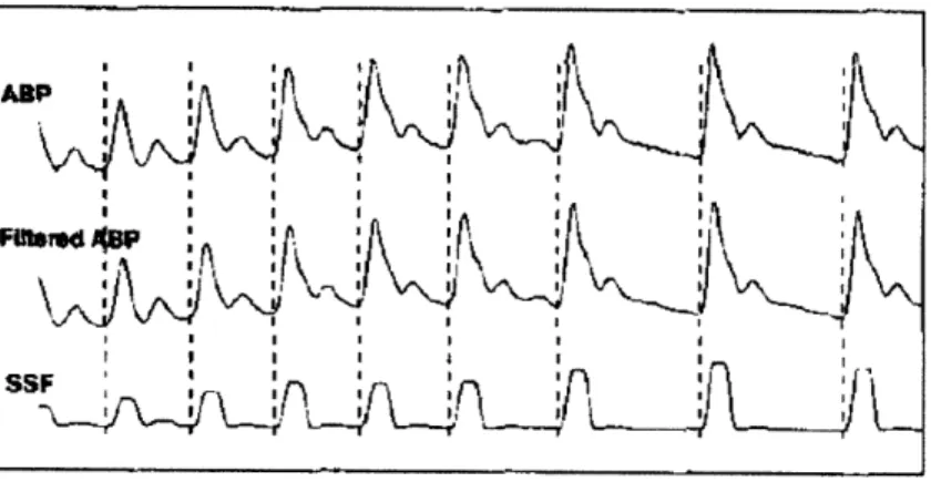
2-6 Beat extraction based on wabp. The SSF function amplifies the rising portion of each beat. ... ... .. .... . . 42

2-7 Distribution of records with thermodilution points taken during peri-ods of clean SQI ... ... . 44

2-8 Thermodilution value distribution. ... 45

2-9 Time in hours between thermodilution measurements. Mean time is 3.1 hours, median time is 2.1 hours, and standard deviation is 8.8 hours. 46 2-10 Case ID a40006 with and without SQI correction. . ... 47

2-11 Estimator comparison at different ABPSQI thresholds. . .. . . . . . 49

2-12 Case ID a40006 with SQI correction . . ... . ... . . 51

2-13 Case ID a40075 with SQI correction. ... 52

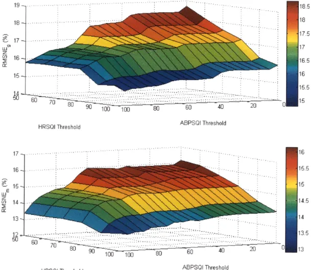
2-14 CO estimation errors at different ABPSQI and HRSQI thresholds using the RMSNE error criteria for the Liljestrand method . . . . . 53

2-15 CO estimation errors at different ABPSQI and HRSQI thresholds using the RMSE error criteria for the Liljestrand method. .. . .. . . . 54

2-16 Data availability at different ABPSQI and HRSQI thresholds ... 55

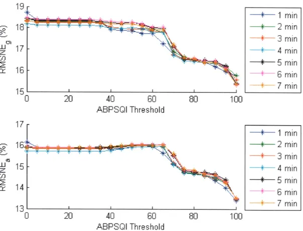
2-17 Effect of window size and ABPSQI threshold on CO estimation error using the Liljestrand method. . ... . 56

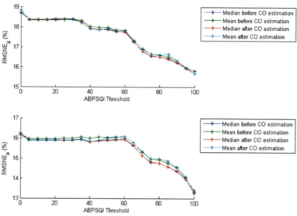
2-18 Effect of performing mean or median operation before and after CO estimation using the Liljestrand method. . ... 57

2-19 Effect of minimum number of good beats in a window . . . . .. . 58

2-20 Calibration constant histogram for Mean Arterial Pressure. ... . . 60

2-21 Calibration constant histogram for Windkessel. . ... .. . . .. 60

2-22 Calibration constant histogram for Liljestrand nonlinear compliance.. 60

2-23 Calibration constant histogram for Herd. . ... 60

2-24 Calibration constant histogram for Systolic area ... . .. 60

2-26 Calibration constant linear regression with thermodilution for Mean

Arterial Pressure. ... ... 61

2-27 Calibration constant linear regression with thermodilution for Wind-kessel ... ... 61

2-28 Calibration constant linear regression with thermodilution for Liljes-trand nonlinear compliance. ... .... 61

2-29 Calibration constant linear regression with thermodilution for Herd. . 61 2-30 Calibration constant linear regression with thermodilution for Systolic area. . ... .. ... ... 61

2-31 Calibration constant linear regression with thermodilution for Wesseling. 61 2-32 Normalized error, EC~TCO) (100%), at a range of thermodilution values. ... ... ... 62

2-33 Absolute error, ECO - TCO, at a range of thermodilution values. .. 63

2-34 RMSNE as a function of heart rate. ... 64

2-35 RMSE as a function of heart rate. ... . 64

2-36 RMSNE as a function of mean ABP. ... 65

2-37 RMSE as a function of mean ABP. ... 65

2-38 RMSNE as a function of pulse pressure. ... ... 66

2-39 RMSE as a function of pulse pressure. ... . ... . 66

2-40 5% bootstrap Mean Square Error (MSE) with raw estimations. The estimators are in the following order: 1) mean arterial pressure, 2) Windkessel, 3) Herd, 4) Liljestrand, 5) Systolic Area, 6) Wesseling, and 7) LC. Errors bars indicate standard deviations over 20 runs. . . 68

3-1 P, ECO, R, and levophed doses for a41244. . ... . . 76

3-2 Distribution of AR and AD for vasoconstrictors for the Liljestrand estimator. The green and red ellipses represent the 2 and 3 standard deviation boundaries of the joint distribution. ... . 78

3-3 Distribution of AR and AD for vasodilators for the Liljestrand es-timator. The green and red ellipses represent the 2 and 3 standard

deviation boundaries of the joint distribution . ... 79

3-4 Distribution of VRP and VD for vasoconstrictors for the Liljestrand estimator. The green and red ellipses represent the 2 and 3 standard

deviation boundaries of the joint distribution. . ... . 79

3-5 Distribution of VR and VD for vasodilators for the Liljestrand es-timator. The green and red ellipses represent the 2 and 3 standard

deviation boundaries of the joint distribution. . ... . 80

3-6 Distribution of AR and AD for vasoconstrictors for the LC estimator. 80 3-7 Distribution of AR and AD for vasodilators for the LC estimator. .. 81 3-8 Distribution of VR and VD for vasoconstrictors for the LC estimator. 81 3-9 Distribution of VP and VD for vasodilators for the LC estimator. .. 82 3-10 Medication changes and corresponding resistance changes for each event,

organized by drug effect, for Liljestrand estimator. . ... 84 3-11 Medication changes and corresponding resistance changes for each event,

organized by medication, for Liljestrand estimator. . ... 84 3-12 Medication changes and corresponding resistance changes for each event,

organized by drug effect, for LC estimator. . ... 85

3-13 Medication changes and corresponding resistance changes for each event,

organized by medication, for LC estimator. . ... . 85

3-14 Medication slopes and corresponding resistance slopes for each event, organized by drug effect for the Liljestrand estimator. . ... 87 3-15 Medication slopes and corresponding resistance slopes for each event,

organized by medication for the Liljestrand estimator... . . 88 3-16 Medication slopes and corresponding resistance slopes for each event,

organized by drug effect for the LC estimator. . ... . 88 3-17 Medication slopes and corresponding resistance slopes for each event,

4-1 Estimated CO, estimated R, HR, and ABP for a41232. Periods of signal quality greater than 90 for HRSQI and ABPSQI are flagged on

their respective plots. ... ... 96

4-2 Estimated CO, estimated R, HR, and ABP for a40694. Periods of signal quality greater than 90 for HRSQI and ABPSQI are flagged on their respective plots. ... ... 97

4-3 Example of artifact from a40694: saturation to mean... . . 98

4-4 Estimated CO, _{estimated R, HR, and ABP for a40542. Periods of} signal quality greater than 90 for HRSQI and ABPSQI are flagged on their respective plots. ... ... 99

4-5 Estimated CO, _{estimated R, HR, and ABP for a40638. Periods of} signal quality greater than 90 for HRSQI and ABPSQI are flagged on their respective plots ... ... ... . 101

4-6 Estimated CO, _{estimated R, HR, and ABP for a41895. Periods of} signal quality greater than 90 for HRSQI and ABPSQI are flagged on their respective plots. ... .... .. . . 102

4-7 Estimated CO, _{estimated R, HR, and ABP for a41681. Periods of} signal quality greater than 90 for HRSQI and ABPSQI are flagged on their respective plots ... .. .. . . .. 103

4-8 Estimated CO, _{estimated R, HR, and ABP for a40968. Thermodilution} is shown in red with error bars of 20%. Periods of signal quality greater than 90 for HRSQI and ABPSQI are flagged on their respective plots. 104 4-9 Example of artifact from a41232: damping and consequent flush. . ... 105

4-10 Proposed damping detection method. ... . 106

4-11 Envelope extraction for a40022. ... . 107

4-12 Envelope extraction for a40022 using the RMS method. ... . 108

4-13 Envelope extraction for a40022 using the Hilbert method ... . 108

List of Tables

1.1 jSQI criteria. ... ... . ... .. 29

2.1 Cardiac output estimators indexed by i. Pm, mean arterial pressure; Pp, pulse pressure; Pd, diastolic arterial pressure; P, systolic arterial pressure; h, heart rate; A₈, area during systole. . ... . 36

2.2 Extracted ABP Features. ... ... 43

2.3 Statistics for calibration constants ki for different estimators at

recom-mended SQI thresholds to remove noisy data. . ... 59

3.1 List of vasoactive medications and their effects on peripheral resistance. 72 3.2 List of ICD-9 codes used to identify patients with septic shock,

cardio-genic shock, and hemorrhage. ... ... 74

3.3 Expected estimated resistance and medication changes. . ... 83 3.4 AR and AD regression results for the Liljestrand estimator. Linear

regression line in the form of y = ax + b. ... ... 86

3.5 AR and AD regression results for the LC estimator. Linear regression

line in the form of y = ax + b. ... ... . . 86

3.6 V/R and VD regression results for the Liljestrand estimator. Linear

regression line in the form of y = ax + b. . ... 87

3.7 VR and VD regression results for the LC estimator. Linear regression

Chapter 1

Introduction

Modern intensive care units (ICUs) measure a large number of physiologic signals that are intended to provide clinicians comprehensive information to diagnose and treat patients. However, the quantity of information can be overwhelming to the clinician and hinder the integration of relevant data crucial to the patient's condition. One of the many signals typically measured in an ICU setting is blood pressure, which can be processed and interpreted to aid clinicians in better tracking of the patient's state.

1.1

Cardiovascular System Background

The major functions of the cardiovascular system are to perfuse the vital organs with blood, provide oxygen to tissues, and distribute essential molecules to the cells while carrying away metabolic waste products to maintain the body's internal environment. As illustrated in Fig.1-1, blood is carried from the heart to the body through the arteries, thick-walled vessels that carry the blood at high pressures. The arteries branch into a series of arterioles, which then in turn branch into capillaries. These capillaries, with their walls only a single layer of cells thick, are the site of exchange of oxygen, carbon dioxide, nutrients, and wastes to and from the tissues. Blood is carried back to the heart through the veins, thin-walled vessels that carry the blood at low pressures. After the blood returns to the right atrium of the heart, it passes into the right ventricle, from which it is ejected into the pulmonary system for gas

exchange. Oxygenated blood returns to the heart and fills the left atrium. Blood then fills the left ventricle, and the left ventricle pumps the blood through the systemic

circulation system.

Cardiac output (CO) is a measure of the amount of blood pumped by either ventricle. In steady state, the outputs of both ventricles are the same. In a healthy adult male, cardiac output is approximately 5 L/min [7]. Cardiac output can vary, however, according to the body's physiological needs; for example, a well-trained athlete, while exercising, can increase cardiac output to up to 30 L/min to increase the rate of transport of oxygen, nutrients, and wastes [13]. Abnormally low levels of cardiac output can also be an indication of pathology.

1.2

Motivation for Cardiac Output Estimation

Cardiac output is one of the most important hemodynamic signals to measure in patients with compromised cardiovascular performance. Fig.1-2 illustrates the sig-nificance of cardiac output monitoring in severe acute hemorrhage, displaying the changes in total peripheral resistance, heart rate, arterial blood pressure, right atrial pressure, and cardiac output during a hemorrhage. Although arterial blood pressure decreases throughout blood loss and drops sharply at approximately 10 minutes after onset of hemorrhage, cardiac filling pressure and cardiac output provide earlier indi-cations of anomalous cardiovascular behavior. This example illustrates the fact that measurements of cardiac output and filling pressure provide information for "early diagnosis, monitoring of disease progression, and titration of therapy in heart fail-ure, shock of any type, sepsis, and during cardiac surgery" [15]. If cardiac output could be measured at more frequent intervals, or even continuously, clinicians could detect abnormalities in the cardiovascular system and execute appropriate interven-tions sooner.

Currently, cardiac output monitoring in the ICU is monitored invasively and only intermittently. In the ICU, the thermodilution cardiac output (TCO) method, in-troduced by Fegler in 1954 [12], has been the "gold standard" commonly used to

Head

(oroiary

=

RSplnich Venrle

Portal Pral Vein

Mesenteric Kidic y

Tubular Gloncrutar RA = Right Atrium

LA = eft Atrium bUgs RV = Right Ventricle

PV = Portal ,ejin

Figure 1-1: Cardiovascular system. Xs indicate local control points. The arterial system is displayed on the right, while the venous system is displayed on the left. Adapted from [29].

Z 20-0. 10 TP.R . /

-z

--200

0

w

cardiac output; RT, right. Adapted ₀₀ m

[3].

s

I-to I*

0 4 8 12 16

MINUTES

Figure 1-2: Example of severe acute hemorrhage starting at t=O. TPR, total periph-eral resistance; HR. heart rate: BP, blood pressure; RAP, right atrial pressure; CO, cardiac output; RT, right,. Adapted from [3].

to CldQ P*Oak EAd Iaqgrtiolo Slow Rsurn

( TmwhenjTo w.iin of Tenp to

Z 01' C ofbs .1ie a8osti,,

-06 %lDW OC8ASELINE FLUCTUATIONS 04- IN TEMP, SYNCHRONOUS " WITH RESPIRATION z 0.2 0 00*C OL 0 10 20 30 40 50 60 seconds

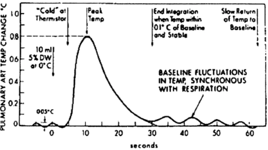
Figure 1-3: Typical thermodilution curve. Baseline fluctuations may reach 0.1 degrees Celsius. Adapted from [31].

measure cardiac output, whereby a bolus of cold solution of saline or dextrose is injected into the right atrium. Temperature change is monitored at the pulmonary artery using a balloon-tipped Swan-Ganz catheter, which involves an invasive proce-dure that requires threading the catheter through the vena cava and the right heart. Using this method, cardiac output is inversely proportional to the integral of the measured temperature curve, as illustrated in Fig.1-3. This method can only be per-formed in well-equipped environments such as ICUs or cardiac catheterization labs. Current invasive procedures for monitoring cardiac output increase the potential for complications, including the higher risk of infection and sepsis, and increase the pos-sibilities of morbidity and mortality [6]. Furthermore, TCO measurements can only be taken intermittently to prevent volume overload and to allow for sufficient time for temperature changes to occur in the bloodstream [20]. Therefore, both patients and clinicians would benefit from having a continuous, non-invasive, reliable method of estimating CO.

Other methods of measuring CO exist, but requires additional measurements, tests, and/or equipment. The Fick method derives CO through calculating oxygen consumed over a given period of time by measuring oxygen consumption per minute with a spirometer, oxygen concentration of venous blood from the pulmonary artery, and oxygen concentration of arterial blood from a peripheral artery. Impedance car-diography is a non-invasive method of measuring CO, whereby electrodes are placed

on the neck and chest to transmit and detect impedance changes in the thorax. Impedance changes are due to changes in intrathoracic fluid volume and respiration, so changes in blood volume per cardiac cycle can be measured and used to estimate stroke volume and CO, but reliability and reproducibility of measurements have been limited [42]. The Doppler ultrasound method uses reflected sound waves to calculate flow velocity and volume to obtain cardiac output and is a non-invasive, accurate way of measuring CO using a handheld transducer placed over the skin.

The precision for thermodilution measurements is approximately ±10-20% (0.5-1 L/min for a standard 5L/mnin cardiac output) with a 95% confidence interval [27, 36]. Studies have shown that measuring cardiac output using thermodilution has little bias compared to existing methods such as the Fick method, but other studies show TCO can also overestimate cardiac output by as much as 2.3 L/min [22, 17, 11]. Furthermore, a variety of factors contribute to error in cardiac output estimation by thermodilution: temperature and volume of injectate, rewarming of injectate, timing of injection and respiration, speed and mode of injection, and intravenous fluid administration, among others [31].

Cardiac output is determined by a variety of factors, including heart rate, stroke volume, venous compliance, total peripheral resistance, blood volume, intrathoracic pressure, and cardiac compliance. Many have developed non-invasive or minimally invasive methods to continuously estimate CO [8, 19]. In particular, the arterial blood pressure (ABP) waveform has generated much interest and research for its use in estimating cardiac output. Not only is ABP a routinely measured signal in ICU settings, but measurements are often continuous and less invasive, providing a source of data for continuous CO estimation. Even if CO estimates from ABP are less accurate than existing methods, the derived CO trends can be a powerful tool for clinicians; for example, decreasing CO may indicate shock, and the effectiveness of therapies can be monitored by examining whether or not CO increases to normal levels. Most importantly, CO estimation using ABP requires little to no additional equipment or personnel if the computational power of the existing bedside monitor is sufficient for the numerical calculations required.

1.3

Arterial Blood Pressure

Arterial blood pressure is regulated by cardiovascular control mechanisms and re-flects the cardiovascular system function. Fig.1-4 illustrates the pressure changes in a typical cardiac cycle during which the heart fills and ejects blood, along with the associated aortic flow, ventricular volume, heart sounds, venous pulse, and electro-cardiogram. The cardiac cycle can be separated into diastolic and systolic phases. During diastole, the ventricles relax and fill with blood, and this phase is approxi-mately two-thirds of the cardiac cycle. During systole, the ventricles contract and pump blood to the pulmonary and systemic systems, creating high pressures in the blood vessels. Diastolic and systolic arterial blood pressures are indicated in Fig.1-5 by Pa and P,, respectively. The pulse pressure P, is the difference between the systolic and diastolic pressures. Mean pressure Pm is the time-averaged arterial blood pres-sure through one cardiac cycle and is approximately equal to the diastolic prespres-sure plus one-third of the pulse pressure. Typical values for systolic and diastolic pres-sures are 120 mmHg and 80 mmHg, respectively, and blood pressure is often written as 120/80.

In an ICU setting, ABP is frequently measured invasively using a pressure trans-ducer connected by a catheter to an artery. The radial artery (or occasionally the femoral artery) is used due to its ease in cannulation and the low incidence of compli-cations [35]. Systolic and pulse pressures are higher in these large arteries than in the aorta, while diastolic and mean pressures are slightly lower downstream. Eventually, as the blood reaches the arterioles, capillaries, venules, and veins, pulse pressure is absent [7]. Blood pressure can also be measured intermittently and noninvasively using an oscillometric system. ABP fluctuates diurnally with a baseline change of approximately 20 mmHg, with blood pressure being lower at night [2]. Since ICU patients are managed for cardiovascular stability with drugs and are almost always supine, ABP and heart rate are much more restricted in range than for active, healthy subjects [21].

C 4J C C V U 4 d _ >? o ~O. e= 4J= S15 '_' Q a~ SLeft ventricular 604 pressure 40- Mitral valve

20 _20I closes Mitral valve

4.opens Left Atrial S 5 Pressure 2 4 - 38-$ 324 26 20 Q Ventricular 0 0.1 0.2 0,3 0.4 0.5 0.6 0.7 0.8 Time (sec)

Figure 1-4: Left atrial, aortic, and left ventricular pressure measurements with asso-ciated aortic flow, ventricular volume, heart sounds, venous pulse, and electrocardio-gram for a complete cardiac cycle in the dog. Adapted from [29].

Pressure 160 (mmHg) PS 140 120 100 PP = Ps - Pd 80 60 ~40 pd : P(t)dt 20 tk+1 - tk tk tk+1 Time

Figure 1-5: Arterial blood pressure from a MIMIC II patient. Adapted from [32].

1.4

MIMIC II Database

The MIT Laboratory of Computational Physiology (LCP) currently collaborates with Philips Healthcare and Beth Israel Deaconess Medical Center in an ongoing effort to collect, develop, and evaluate ICU patient monitoring systems that will improve clin-ical decision-making. As part of this collaboration, the lab has developed the Multi-Parameter Intelligent Patient Monitoring for Intensive Care (MIMIC) II database, an online database that contains more than 30,000 de-identified records from patients hospitalized at the Beth Israel Deaconess Medical Center in Boston, Massachusetts [34] [5]. More than 4,000 of these records contain physiological data including bedside waveform and physiological trend data. Waveform data are sampled at 125 Hz with 8 or 10 bit resolution and typically include multichannel electrocardiogram traces, arte-rial blood pressure measurements, central venous pressure waveforms, and pulmonary artery pressure waveforms. Trend data, which are derived from the waveforms, are collected only intermittently and are usually recorded at a rate of 1 sample/min. De-rived trends include heart rate, mean, systolic, and diastolic arterial pressure, mean, systolic, and diastolic pulmonary artery pressure, and cardiac output (using ther-modilution). Currently, the public MIMIC II database includes 1710 ICU stays with

arterial blood pressure waveform and derived measurements, totaling approximately 104,000 hours of data. The database contains 282 trend records with thermodilution measurements, which are measured intermittently. Of these data, 265 patient records contain both arterial blood pressure and thermodilution measurements, totaling 2754 TCO measurements.

1.5

ABP Signal Quality Index

ABP waveform data are prone to artifacts due to patient movement, sensor discon-nections, arterial line blockage, or mechanical devices such as intra-aortic balloon pumps. Because the accuracy of CO estimates based on analysis of ABP waveforms is a function of the quality of the ABP waveform, a systematic method needs to be used to remove artifacts or abnormal (non-sinus rhythm) ABP beats. Previous liter-ature has defined signal quality indices (SQI) for both blood pressure and heart rate based on MIMIC II data [25, 24, 37, 44]. For blood pressure signal quality, Li et al combined two independent signal quality assessment methods, jSQI [38] and wSQI

[44] to form ABPSQI. For both signal quality metrics, beat extraction is performed using wabp, an open-source ABP onset detection algorithm [43].

The jSQI algorithm examines each beat, extracting a series of inter- and intra-beat features and comparing them to a set of maximum or minimum values that are beyond the physiological range. Beats that fail any one of these criteria are flagged as "bad". Table 1.1 provides a list of these features and associated thresholds beyond which a beat is considered abnormal. For each beat, systolic and diastolic pressures are the local maximum and minimum values within the duration of the beat, while the beat duration is the time difference between adjacent onsets. The first 4 criteria in Table 1.1 impose bounds on the physiologic ranges of each feature. For example, systolic pressures above 300 mmHg are flagged as abnormal. The noise level, w, is defined as the average of all negative slopes in each beat, so high frequency noise, which often contains large negative slopes, is detected. This method of noise detec-tion does not identify low frequency noise such as baseline wander and is dependent

on the sampling frequency (125 Hz for the MIMIC II database), since this is a gra-dient calculation for each sample in a beat. The last 3 criteria in Table 1.1 examine variations between adjacent beats.

Feature Abnormality criteria

Ps Ps > 300 mmHg Pd Pd < 20 mmHg Pm, P, < 30 or P > 200 mmHg HR HR < 20 or HR > 200 bpm P, Pp < 20 mmHg w w < -40 mmHg / 100 ms PT[k] - P[k - 1] AP I > 20 mmHg Pd[k] - Pd[k - 1] XAPdl > 20 mmHg T[k] - T[k - 1] IATJ > 2/3 sec

Table 1.1: jSQI criteria. Pm, mean arterial pressure; Pd, diastolic arterial pressure; P, systolic arterial pressure; T, beat duration; HR, instantaneous heart rate as calculated by 60/T; Pp, pulse pressure; w, noise: mean of negative slopes. Adapted from [38].

jSQI is an abnormality index and produces a binary number for each beat with 0 equating to normality and 1 abnormality. Note that an abnormal rating may be due to artifacts or pathophysiology such as an arrhythmia or balloon pump. In Fig.1-6, for example, the abnormal regions are indicated by the two red shaded regions on the x-axis. The final beat in the second abnormal section ending at approximately 25 seconds is labeled as abnormal even though it appears normal because jSQI compares this beat to the previously detected beat and looks for similarities. Compared to human annotation, jSQI has a sensitivity of 1.00 and a positive predictivity of 0.91

[38].

The wSQI algorithm extracts beat by beat features from ABP, expresses the features using fuzzy representation, and uses a fuzzy reasoning procedure, outlined in Fig.1-7, to produce a continuous SQI between 0 and 1, where 1 is the best signal quality. The features used for this algorithm are systolic blood pressure, diastolic blood pressure, mean blood pressure, maximum positive pressure slope, maximum negative pressure slope, maximum up-slope duration (the maximum duration that the ABP signal continues to rise), maximum duration above threshold (the maximum

Vi I, 150 - 0 0 0 5 10 15 20 25 time Iseconds

Figure 1-6: A clinical ABP waveform with jSQI designated at the bottom, flagging regions of abnormality. Adapted from [38].

[01 &M ABP

to = (prvos) t1 i

duration that the ABP signal stays above a threshold), pulsee-to-pulse interval, pulse pressure, and ECG-ABP delay time (the interval between _Yes th Qe QShEG

and the onulset of the following ABP pulse). Fig.-8 illustrates the output from this_{onset times are compared to those extracted from the EG signal and thresholded.} The wSQI algorithm has been shown to have a sensitivity of 99.8% and a positive_{NoA ABP pub tisnang}

&8 Funuing _{SW' =0}

SQ

Figure 1-7: Outline of wSQI procedure. wSQI uses fuzzy logic and fuzzy reprentation to determine a signal quality metrindexic ABP (Ablood pressure. to and tI are thefor start and end times of each blood pressure pulse. Adapted from [44].

duration that the ABP signal stays above a threshold), pulse-to-pulse interval, pulse pressure, and ECG-ABP delay time (the interval between the QRS onset in the ECG and the onset of the following ABP pulse). Fig.1-8 illustrates the output from this algorithm. If an electrocardiogram (ECG) signal is available, detected ABP beat onset times are compared to those extracted from the ECG signal and thresholded. The wSQI algorithm has been shown to have a sensitivity of 99.8% and a positive predictivity of 99.3% on data from the MIMIC I Database, an earlier multiparamter ICU database. wSQI values above 0.5 correspond to good ABP signal quality [44].

To form a signal quality metric for ABP (ABPSQI), Li et al combined jSQI and wSQI using the following method:

ABPSQI = wSQI if jSQI = 0;ABP

SQl

0 4:46:58 4-4T281

Figure 1-8: Clinical ABP and ECG waveforms with wSQI designated at the bottom. Note that wSQJ lags one beat behind waveforms. Adapted from [44].

ABPSQI={ w QI if.'SQI - 0;

wSQI * q if jSQI = 1.

where 1 is an arbitrary weight that was set to be 0.7.

1.6

HR Estimation and

HRSQI

For the CO estimators analyzed in this thesis, blood pressure features are used to estimate stroke volume, which is then is multiplied by heart rate to derive cardiac output. Therefore, reliable heart rate measurements are also an integral component for deriving reliable CO estimates.

Li et al [25] developed a method for robust heart rate estimation by fusing heart rate estimates derived from ABP and ECG. Heart rate is extracted from multiple ECG leads using a weighted Kalman filter to produce a robust heart rate estimate. Meanwhile, ABP heart rate is calculated from ABP waveforms based on beat onset times from wabp. HR estimates from both ECG and ABP are tracked with separate Kalman filters that used SQI-weighted update sequences. A fused heart rate is derived by weighting each HR estimate by the SQI-weighted residual errors of each Kalman filter for each HR time series.

For each fused segment, a corresponding signal quality (HRSQI) is computed to indicate its reliability. HRSQI is composed of 2 SQIs: ABPSQI (described in Section

1g 100 1 0 0 83 6 7S 6 S 7 7 7 7T N T W7? S rG 76 M 0 75 S 30 I I I I I t I I I I S1 1 1 1 0I 00 1' 0 1 0 0 000 0 1 i 000 I I I I 0 0 0 I 1 1 36( 0 0 3 2 SS 65 b e 30 (a) (b) (C) (d) (e)

Figure 1-9: A two-lead ECG waveform and corresponding ECG SQI. ECGSQI is derived from combining several quality indices related to beat detecton (bSQI), inter-channel agreement (iSQI), Gassianity (kSQI), and spectral coherence (sSQI). Adapted from [25].

1.5) and ECGSQI. ECGSQI is the signal quality of the ECG heart rate estimation method used to derive the heart rate component from ECG. ECGSQI is formed based on a variety of factors: the comparison of multiple beat detection algorithms on a single lead, beat detection comparison using different ECG leads, kurtosis of the ECG, and spectral distribution of ECG. Fig.1-9 illustrates the ECGSQI on a short section of multi-lead ECG. An ECGSQI value between between 0 and 1 is assigned to the corresponding HR estimates as a metric for the reliability of the ECG-derived HR. ECGSQIs greater than 0.5 indicate a signal from which a fair estimate of HR can be derived, with ECGSQIs greater than 0.7 generally providing an excellent HR estimate.

The reliability of the fused HR is indicated by a composite signal quality measure HRSQI using the following method:

1.7

Project Scope and Goals

This thesis compares and evaluates the accuracy of CO estimators that use ABP waveform data, using thermodilution measurements of CO as the gold standard. Trends in CO are then related to physiological changes to determine the clinical usefulness of the estimates. The first part of this thesis evaluates and compares the performance of 6 CO estimators on data from MIMIC II, incorporating heart rate, blood pressure, and their corresponding signal quality indices in the estimation process. The accuracies of CO estimates are then compared with thermodilution measurements in the MIMIC II database. Estimated CO errors as a function of estimated CO, heart rate, mean blood pressure, and pulse pressure are also explored. The second part of this thesis attempts to evaluate the clinical usefulness of CO estimates by analyzing correlations between the administration of vasoactive pressors and the measured and calculated hemodynamics. That is, cardiac output, peripheral resistance (R), and mean arterial blood pressure should change over time following drug delivery. Administration of vasoconstrictors results in an increased peripheral resistance, which is the ratio between mean ABP and cardiac output, while vasodila-tors result in a decreased peripheral resistance. Estimated peripheral resistance (R) is calculated by dividing the mean ABP by estimated CO. By examining changes in fR at the vicinity of a stop, start, or significant change in pressor dose, we may evaluate the utility of these estimates in a real-world setting.

Chapter 2

Cardiac Output Estimation

The goal of this section is to produce reliable cardiac output estimates based on blood pressure waveform data. This requires 3 essential components:

1. Reliable ABP measurements 2. Reliable HR measurements

3. An accurate CO estimator method

The CO estimates were evaluated on records from the MIMIC II database [5] with simulataneous ABP waveform & TCO recordings. Patients with intra-aortic balloon pumps or fewer than 5 TCO measurements were not included in the analysis, as con-sistent with previous literature [37] [39] to provide sufficient calibration points. These restrictions provide 1,497 thermodilution measurements from 121 records for calibra-tion. Thermodilution was used as the gold standard against which the estimated CO was compared.

2.1

Cardiac Output Estimation Theory

A variety of cardiac output estimators have been developed over the past hundred years. The estimators evaluated in this thesis rely on circuit models or pressure-area methods to estimate stroke volume and use heart rate to obtain cardiac output.

A superset of these cardiac output estimators have been evaluated by Sun [37] but focused solely on the use of jSQI for a signal quality metric. The CO estimators evaluated in this study are listed in Table 2.1. The proportionality constant reflects arterial compliance and peripheral resistance factors that may not be calculated using arterial blood pressure waveforms without additional calibration data. The estimators are broken into two general groups by a horizontal line. The first set of estimators are based on lumped-parameter models for cardiovascular circulation. The second set of estimators are based on systolic-area methods.

i CO estimator CO = k. -belo.w

1 Mean arterial pressure P,,

2 Windkessel [10] P,. h

3 Liljestrand nonlinear compliance [26] P P . h

4 Herd [16] (Pm, - Pd) .h

5 Systolic area [40] A8 " h

6 VWesseling [41] (163 + h - 0.48 - Pm,) -A - h

Table 2.1: Cardiac output estimators indexed by i. Pm, _{mean arterial pressure; P,} pulse pressure; Pf, diastolic arterial pressure; P, _{systolic arterial pressure; h, heart} rate; A, area during systole.

2.1.1

Lumped-Parameter Models

Electrical circuits have been used to model the relationship between CO and ABP, and a number of lumped-parameter models of various complexities have been developed to model circulation. Current is analogous to flow (Q), while voltage is analogous to pressure (P). In the case of circulation, flow is equal to CO, so Q and CO can be used interchangeably.

Method 1: Mean arterial pressure (MAP)

The viscous flow of blood through blood vessels contributes resistance to blood flow, and the determinants of resistance include blood viscosity and radius of the blood vessel. The blood vessels throughout the body can be modeled as resistors in parallel or series. Peripheral resistance (R) is the total equivalent resistance of blood flow

Figure 2-1: Mean arterial pressure model. P,, mean arterial pressure; R, peripheral resistance; Q cardiac output.

throughout the body. The mean arterial pressure model takes into account peripheral resistance, mainly contributed from arterioles, and models the heart using a current source Q as illustrated in Fig.2-1. This circuit analogy is valid only for time-averaged flow and not intra-beat fluctuations. CO is computed using Ohm's law as follows:

Q = ki -Pm

where Pm is the mean arterial pressure, R is the peripheral resistance, and k, = J.

Method 2: Windkessel

The Windkessel model [10], shown in Fig.2-2, describes the pulsatile phenomenon of arterial blood pressure. As with the mean arterial pressure model, the resistor component corresponds to the resistance of the systemic blood vessels. The capacitor models the compliance of the arteries, which inherently store some blood during the cardiac cycle. Compliance (C) is a measure of the distensibility of the blood vessels, and the capacitor represents the aggregate elastic properties of the systemic peripheral system:

AV

C =

AP

where V represents the volume of blood and P the transmural pressure across the wall of the blood vessel. The heart is modeled by a time-varying current source Q(t) representing blood flow, and each beat of the heart corresponds to an impulse with an area equal to the stroke volume (SV), the amount of blood pumped per beat, such

Figure 2-2: Windkessel model. P (t), arterial pressure; R, peripheral resistance;

Q

that:

Q

(t)=

SV.6

(t

-

where n is the n'_{h beat over which Q}

is calculated, t,, is the time of the Ih' beat, and

SV, is the stroke volume due to the nh beat. The resulting pressure waveform exhibits an exponential decay after each beat within the RC time constant and resembles the physiological arterial pressure waveform, particularly during diastole. The state space equation for the Windkessel model is:

dP (t) P (t)

C

+

= Q (t)

where C is the arterial compliance. By circuit analysis, stroke volume is proportional to the pulse pressure, P, (the amplitude range of the ABP waveform); heart rate, h; and the compliance, C in steady state such that:

Q = k2 -P,-h1

where k2 -= C

Method 3: Liljestrand nonlinear compliance

Compliance varies throughout the cardiac cycle and is dependent on arterial pressure. When pressure increases during systole, blood vessels expand and become stiffer, de-creasing incremental compliance. This CO estimator uses a pressure-varying capacitor

(7)if}i

Figure 2-3: Liljestrand nonlinear compliance model. Compliance varies according to systolic and diastolic pressure. P (t), arterial pressure; R, peripheral resistance; Q (t) cardiac output; C compliance.

C = k to correct for this nonlinearity, as seen in Fig.2-3 [26]:

PP, + Pd

k3

Q = Ps + Pd .Pp" h

where k3 is an arbitrary constant derived from a measurement of cardiac output using

an independent method such as Fick's or thermodilution.

Method 4: Herd

Herd empirically observed that Pm- Pd is proportional to stroke volume [16]. There is no physiological intuition for this assumption, but it corrects for varying compliance, with decreasing compliance as pressure increases. Cardiac output is therefore:

Q =

2.1.2

Pressure-Area Methods

Another approach to cardiac output estimation using blood pressure is by approaching the arterial tree from a distributed systems point of view. More specifically, systolic area can be correlated with stroke volume to obtain an estimated CO.

Method 5: Systolic area

As illustrated in Fig.2-4, the area under the systole region, As, of the ABP waveform is proportional to the stroke volume [40]. Systolic area is proportional to the amount

o

---Figure 2-4: Systolic area estimation. Stroke volume is proportional to the area of the shaded region, P, = A,. T, and Td represent the durations of the systolic and diastolic phases of the beat. Adapted from [23].

of blood drained from the peripheral vasculature; a longer systole or higher systolic pressures reflect a greater volume of blood the heart must eject. CO can be calculated as follows:

Q= k- A, h

Method 6: Wesseling

Wesseling et al applied a correction factor to the systolic area method described above to take into account non-negligible contribution of fluctuations in ABP during systole [41]. Based on empirical studies and optimal linear regression analysis, impedance is corrected for to calculate CO:

Q

2.2

Evaluation Procedure

The cardiac output estimation and evaluation procedure is outlined in Fig.2-5. First, appropriate ABP data were extracted from records in the MIMIC II database, in-cluding 10-second trend files (T-files) that include a blood pressure SQI metric, fused heart rate from ABP and ECG, and a heart rate SQI metric generated by Li et al [25]. Then, appropriate blood pressure features were extracted and used to

deter-(1) Database-specific processing

I

--"

,-- ,

(4) CO Estimation

CO Calibration with eCO Performance

Estimator

Thermodilution

Evaluation

Figure 2-5: Cardiac output estimation and evaluation procedure. ABP and ther-modilution data was first extracted from the MIMIC II database. Relevant features of the blood pressure waveform were extracted after segmenting the waveform into beats. The HR and ABP SQIs of each beat were compared for each window, and if the number of beats that satisfy SQI requirements was sufficient, a CO estimate was made for the window. After the estimated CO was computed for the entire record, CO was calibrated with thermodilution measurements, and the difference between the estimated CO and thermodilution was analyzed for performance evaluation.

mine whether each window contains sufficiently clean ABP and HR to generate a CO estimate. After CO estimates were generated for the record, the CO estimate was calibrated with thermodilution measurements. To evaluate the performance of the CO estimation procedure, estimated CO and measured thermodilution (TCO) were compared.

2.2.1

Database-specific processing

Relevant source code: wavex2.m, Tex.m, trendex2.m

From the MIMIC II Database, 121 records were identified with simultaneously

Figure 2-6: Beat extraction based on wabp. The SSF function amplifies the rising portion of each beat. Adapted from [43].

available ABP waveforms and TCO measurements. The ABP waveforms were mea-sured from the femoral or radial arteries and sampled at 125 Hz with 8-bit quantiza-tion. TCO was available intermittently with a temporal resolution of 1 minute.

Trend files contain fused HR,, HRSQI, and ABPSQI from previous analysis of heart rate estimation on MIMIC II data [25] at 10-second intervals. The derivation of the fused HR, HRSQI, and ABPSQI from ECG and ABP waveforms are described in Sections 1.5 and 1.6. From this point forward in this chapter, the fused HR developed will be referred to when mentioning heart rate.

2.2.2

Feature extraction

Relevant source code: wabp.m, abpfeature.m

Each ABP beat was extracted from the ABP waveform. A Matlab implementation of Zong et al's wabp algorithm [43] detects the onset of each beat using a slope sum function (SSF), which is a representation of the rising portions of each beat. An example is shown in Fig.2-6. A decision rule based on adaptive thresholds and searching strategies determines whether or not an onset is detected.

After the waveform was segmented into beats, important features for each beat were extracted. A list of features are included in Table 2.2. The feature extraction algorithm was based on previous work by Sun [37]. For each beat, the local maximum and minimum values correspond to systolic and diastolic blood pressures, respectively.

I I ~ I In . i I i nl I I r I I I _{I~~ I} I I I ' Il ii I 4 I I I I I I _I I _I I _I I _I I I_{I I}

ss

, ,

, , ,n ,

?,

,/

,

:fY4P

Pulse pressure is the difference between the two. Mean pressure is the time average of all pressure samples within the beat between adjacent onsets. The duration of the beat is the time difference between adjacent onsets. The time of the systolic portion of the beat is approximated as T, = 0.3 F [4], and pressure area during systole is

calculated as the area during this time between the instantaneous blood pressure and diastolic pressure for that beat:

A. = f (P(t) Pd)dt

Feature Description Units

P Systolic blood pressure mmHg

Pd Diastolic blood pressure mmHg

Pm Mean blood pressure mmHg

P, Pulse pressure (P, - Pd) mmHg

A, Pressure area during systole mmHg . time

T Duration of each beat sec

Table 2.2: Extracted ABP Features.

2.2.3

SQI Correction

Relevant source code: findgoodbeats.m

A cardiac output estimate was produced for each window with reliable ABP and HR data. Each window was chosen as a minute preceding each TCO measurement, since the invasive nature of the thermodilution technique may change heart rate and blood pressure [31]. The length of the window is consistent with previous litera-ture [37] [39] and was a trade-off between obtaining enough beats for an accurate representation of the hemodynamic condition prior to the measurement, and the nonstationarity of the patient's condition.

Signal quality indices were used as metrics to determine whether or not beats were sufficiently clean for estimation. HR, HRSQI, and ABPSQI from the T-files were linearly interpolated for each beat. For a beat to be considered "good", both heart rate and blood pressure had to pass SQI thresholds such that HRSQI > HRSQIthresh

25 20 15 10 5 5 10 15 20 25 30 35 40 #TCO

Figure 2-7: Distribution of records with thermodilution points taken during periods of clean SQI.

and ABPSQI > ABPSQIthresh. HRSQIthresh and ABPSQIthresh were varied, and their

effects on CO estimator accuracy are discussed in Section 2.3. Likewise, the window size was also varied from 1 second to 7 minutes to examine how CO estimation

accuracy changes.

Within each window preceding TCO measurement, a minimum number of clean beats were required to generate a CO estimate. This minimum was winthresh, which

was empirically set to 6 beats, or approximately 10% of the beats within a 1 minute window. The effects of varying this threshold are explored in Section 2.3. The distribution of records with thermodilution points taken during areas of clean SQI is shown in Fig.2-7, and the distribution of thermodilution values is in Fig.2-8.

2.2.4

CO

Estimation

Relevant source code: estA_B.m, where A is the estimator number and B is the

estimator name (such as est04_Herd.m)

If a window contained sufficient "good" beats, an uncalibrated cardiac output estimate was calculated, using the medians of the beat-by-beat HR and ABP features

350 300 250 200 150 100 50 1 2 3 4 5 6 7 8 9 10 11 12 TCO (L~nin)

Figure 2-8: Thermodilution value distribution.

for beats passing SQI threshold tests. Beats that did not pass both the HR and ABP SQI threshold tests were not included in determining CO. The CO estimators explored were described in Section 2.1.

To account for arterial compliance and peripheral resistance factors, the CO es-timate for a record needs to be calibrated with thermodilution measurements. An optimal calibration method was applied using all available thermodilution points for which CO estimates were produced, and the time between thermodilution measure-ments for the 121 cases considered in this study is shown in Fig.2-9. The calibration method is a least squares estimate between thermodilution and uncalibrated cardiac output. We now define x as the uncalibrated cardiac output (UCO), y as the cali-brated estimated cardiac output (ECO), r _{as the thermodilution measurement (TCO),}

and k as the calibration constant. For a record containing n TCO measurements, the calibration constant was calculated as follows:

0.4 0.3 0.2 0.1 0 5 10 15 20 25 30 35 40 45 50 Time (hours)

Figure 2-9: Time in hours between thermodilution measurements. Mean time is 3.1 hours, median time is 2.1 hours, and standard deviation is 8.8 hours.

TCO UCO ECO r = [r1T2 ' ]' x = [X1X2 ... ' y = kx r'x x'x

After calibration, the calibrated cardiac output was compared to thermodilution. An example is shown in Fig.2-10, where the beige plot is the estimated CO before SQI correction, green plot is estimated CO after SQI correction, the black triangles are the estimated CO within the window preceding each TCO point, and the red circles represent TCO points with error bars of 20%.

-6-0 500 1000 1500 2000 2500

time (min)

Figure 2-10: Case ID a40006 without SQI correction using the Liljestrand CO esti-mation method. The beige plot is the estimated CO before SQI correction, green plot is the estimated CO after SQI correction, the black triangles are the medians of the good beats within the window preceding the TCO point, and the red circles represent TCO points with error bars of 20%.

2.3

Results

2.3.1

Error Criteria

CO estimates were compared to thermodilution measurements to determine the accu-racy of the estimates. A root mean square normalized error (RMSNE) criterion was used, consistent with other CO evaluation studies [32]. Errors were calculated when at least 5 TCO were made during areas of good SQI. For each subject s with n, com-parable thermodilution points, the RMSNE for the ECO for the subject, RMSNES,

is:

1 n (100(TCOi _{- ECOi) 2}

RMSNES = , 1 < s < S

\

where S is 121, the total number of records.

To evaluate the accuracy of the estimates across all subjects, the RMSNEss were averaged to obtain an average RMSNE, RMSNEa. The data set has a total of N comparable thermodilution points across all records:

S

N= Ens

s=1