HAL Id: hal-00592079
https://hal.archives-ouvertes.fr/hal-00592079
Preprint submitted on 11 May 2011
HAL is a multi-disciplinary open access
archive for the deposit and dissemination of
sci-entific research documents, whether they are
pub-lished or not. The documents may come from
teaching and research institutions in France or
abroad, or from public or private research centers.
L’archive ouverte pluridisciplinaire HAL, est
destinée au dépôt et à la diffusion de documents
scientifiques de niveau recherche, publiés ou non,
émanant des établissements d’enseignement et de
recherche français ou étrangers, des laboratoires
publics ou privés.
Consistant velocity-pressure coupling for second-order
L2-penalty and direct-forcing methods
Arthur Sarthou, Stéphane Vincent, Jean-Paul Caltagirone
To cite this version:
Arthur Sarthou, Stéphane Vincent, Jean-Paul Caltagirone. Consistant velocity-pressure coupling for
second-order L2-penalty and direct-forcing methods. 2011. �hal-00592079�
Consistant velocity-pressure coupling for second-order
L
2
-penalty and direct-forcing methods
Arthur Sarthou1, Stéphane Vincent2, Jean-Paul Caltagirone2
Abstract
The present work studies the interactions between fictitious-domain methods on structured grids and velocity-pressure coupling for the resolution of the Navier-Stokes equations. The velocity-pressure-correction approaches are mainly used in this context but the corrector step is generally not modified consistently to take into account the fictitious domain. A consistent modification of the pressure-projection for a high-order penalty (or penalization) method close to the Hikeno-Kajishima modification for the Immersed Boundary Method is presented here. Com-pared to the first-order correction required for the L2-penalty methods, the small values of the penalty parameters do not lead to numerical instabilities in solving the Poisson equation. A comparison of the corrected rotational pressure-correction method with the augmented Lagrangian approach which does not require a correction is car-ried out.
Keywords:Navier-Stokes equations, Fictitious domain, Velocity-pressure coupling, Augmented Lagrangian, Pressure-correction methods, Projection methods, Fractionnal-step methods, Penalty method, Penalization method, Immersed boundary method, Incompressible flows.
1
Introduction
The simulation of real heat and mass transfers often implies interactions between multiphase flows and complex obstacles. Many simulation codes based on structured grids have shown their ability to deal with a large amount of physical phenomena. However, structured grids can not generally match complex interfaces due to their lack of flexibility, and the treatment of problems with complex shapes is unnatural and uneasy with this approach. The fictitious-domain methods have been designed to improve the performances of structured grid codes when complex shapes are necessary. A wide literature has been devoted to the subject during the last decades, especially the last 15 years with the emergence of high-order methods (see for a review [MI05, Sar09]).
A first approach to deal with immersed boundaries is the Distributed Lagrangian Multiplier method proposed by Glowinski [GPHJ99]. Used for the Navier-Stokes equations with finite-element methods, the coupling between fluid and solid media is ensured with Lagrange multipliers introduced into the weak formulation of the Navier-Stokes equations.
Cartesian grid methods [JC98, MCJ01] propose to use structured grid in the whole domain except near obstacles where unstructured cells are created from structured cells. The implementation of the method is not simple due to the numerous different space configurations of the intersections between cells and objects. The existence of small cells can induce solver trouble and need a special treatment.
The Immersed Boundary Method (IBM) was initially presented by Peskin [Pes72, Pes02]. Fictitious boundaries are taken into account through a source term activated only near the boundaries. As the source term is weighted with a discrete Dirac function with a non-zero support, the interface influence is spread over some grid cells and a first order of spatial convergence is generally obtained. Another class of IBM, the Direct-forcing (DF) methods, was initially proposed by Mohd-Yusof [Moh97]. The idea here is to impose a no-slip condition directly on the boundary using a mirrored flow over the boundary. In [FVOMY00, VIFO01], the correct boundary velocity is obtained by interpolating the solution on the boundary and far from the boundary on grid points in the near vicinity
1[email protected], Institut de Mécanique des Fluides de Toulouse, UMR CNRS 5502, INPT, UPS; 1 Allée Camille Soula, 31400 Toulouse, France
of the interface. In [TF03], Tseng and Ferziger use the same principle but extrapolate the solution in ghost cells inside the boundary. This approach can be seen as a generalization of the mirror boundary condition used with the Cartesian staggered grid to impose Dirichlet condition on pressure nodes. As the original conservation equations are solved one node closer to the boundary this approach seems to be more accurate than [FVOMY00, VIFO01].
Originally presented in [Arq84] for the conservation equations, the penalty (or from the french designation, penalization) methods for fictitious domains consist in adding specific terms in the conservation equations to play with the order of magnitude of existing physical contributions so as to obtain at the same time and with the same set of equations various physical properties. The Volume Penalty Method (VPM, [KAPC00] and the references therein) is a simple way to impose a solution in a part of the numerical domain. The methods imposing the solution are called the L2-penalty methods while the H1-penalty methods allows a derivative of the solution to be imposed [ABF99]. Classical penalty methods are of first order only since they consider the projected shape of the interface on the Eulerian grid to define the penalty parameters [RAB07]. In [SVCA08, SVAC08], Sarthou et al. have extended penalty methods to higher orders by modifying the expression of the penalty term using implicit interpolations as in [TF03]. The method is called the Sub-mesh penalty method (SMPM) and has been applied first to elliptic equations. For the Navier-Stokes equations, the incompressibility of the flows has been ensured with an augmented Lagrangian velocity-pressure coupling [FG82, VSC]. This method consists in solving the momentum equation with an augmented Lagrangian term which enforces the divergence-free constraint during an iterative process. Hence, the fulfilment of both incompressibility and boundary constraints is obtained with the resolution of a unique equation.
An issue occurs with the pressure-correction methods as the resolution of an additional elliptic equation is performed to rise a pressure and to obtain a solenoidal field. The IBM for the Navier-Stokes equations are generally used with the pressure-correction methods and modify the predictor step only (where the momentum equation is solved). As no modification of the corrector step is performed, the additional boundary constraint is not taken into account in the final velocity and pressure fields and is then no more respected.
In [Dom08], Domenichini analyzes in details the application of the DF-IBM to the fractional step solution of the Navier-Stokes equations. To focus on the error induced by the non-consistant application of the immersed boundary condition, a spectral solver is used. As can be expected, he notices that the boundary condition is not accurately imposed, even if sub-iterations of the time-splitting can be performed to reduce this error.
This problem is not frequently tackled in the literature and fully satisfactory solutions have been found only recently. In [KKC01], authors use a mass source and sink term in the pressure equation to preserve the mass balance in the boundary cells but the desired velocity is not exactly imposed on the wall. More recently, Taira and Colonius [TC07] consider both the boundary forcing of the Peskin IBM and the pressure as Lagrange multipliers. Hence, the time-splitting procedure is applied in the same time and in an equal manner to both quantities. It allows the rigid body and the incompressibility constraints to be satisfied at the same time.
In [IK07], Ikeno and Kajishima propose a consistant correction for a second-order DF-IBM. The principle is to add the boundary term in the projection step in a consistant way. The update equation of the velocity has to be modified too.
Concerning the L2-penalty methods, a solution for the first-order method is recalled in [PAC08]. However, applying this modification to a high-order method is quite more challenging. Recently, the correction of [IK07] has been applied successfully to the SMPM [Sar09]. A correction for a direct-forcing penalty method has been introduced by Belliard et al. [BF10].
A consistant correction for a fully implicit high-order L2-penalty method is proposed here. The formulation is
derived from the penalized momentum equation and thus naturally obtained. Compared to [BF10], all steps of the method take into account the high-order of the penalty term.
The method is applied to the incremental Goda[God78] and rotational [TMV96] pressure-projection methods coupled with the SMPM. These approaches are compared in time and space to the augmented Lagrangian method. In Section 2, the conservation equations and their discretization are presented. Then, the SMPM is described. The third Section focuses on the consistant correction for the time-splitting methods. In Section 4, numerical tests are performed to study and compare the numerical convergence of the method. The last section concludes the article with a discussion and perspectives are drawn.
2
Governing equations and base discretization
2.1
Governing equations
We consider the following form of the incompressible Navier-Stokes equations in a domain Ω:
∇ · u = 0 (1) ρ ( ∂u ∂t + (u· ∇)u ) =−∇p + ∇ · [µ(∇u + ∇Tu)] (2)
with u the velocity, ρ the variable fluid density, p the pressure, g the gravity vector, and µ the dynamic viscosity. The Navier-Stokes equations are discretized with implicit finite-volumes on a staggered Cartesian grid. A order centered scheme is used to approximate the spatial derivatives while first-order Euler and second-order Gear schemes are used for the time integration. All the terms are written at time (n + 1)∆t, ∆t being the time-step, except for the non-linear term un+1· ∇un+1which is linearized as un· ∇un+1for the first-order Gear scheme and as (2un− un−1)· ∇un+1for the second-order Gear scheme. The modified semi-discrete form of the
original equation (2) is then
ρ ( γ1un+1+ γ2un+ γ3un−1 ∆t + ( (γ4un+ γ5un−1)· ∇ ) un+1 ) =−∇(γ4pn+ γ 5pn−1) +∇ · [µ(∇un+1+∇Tun+1)] (3)
with the additional constraint∇ · un+1= 0. The values of γ
idepend on the temporal scheme as
• γ1= 1, γ2=−1, γ3= 0, γ4= 1, γ5= 0 for the Gear 1 or Euler scheme • γ1= 32, γ2=−2, γ3=12, γ4= 2, γ5=−1 for the Gear 2 scheme.
In the next parts, the Euler scheme is generally written for the sake of simplicity.
The linear system resulting from the discretization is solved with a BiCG-Stab II solver [Gus78], precondi-tioned by a Modified and Incomplete LU method [Vor92].
2.2
The velocity-pressure coupling
2.2.1 Pressure-correction methods
Most of the finite-volume CFD codes on Eulerian grids use pressure-correction (or fractional-step) methods. The idea is to obtain first a predicted velocity u∗satisfying the momentum equation only. This field is not solenoidal as nothing constrains this condition. In a second step, the projection, the pressure is risen with respect to the divergence of u∗. The third step consists in updating the velocity according to the pressure gradient obtained with the second step.
We consider RHS the sum of the convective and diffusive terms of the equation (2). The half discretization in time gives: ρ ( un+1− un ∆t ) = RHSn+1− ∇pn+1. (4) This equation is solved, but as here∇·un+1̸= 0, the solution is denoted u∗. We define u′such as un+1= u′+u∗
and p′such as pn+1= p′+ p∗. Hence, the predictor step solves:
ρ ( u∗− un ∆t ) = RHS∗− ∇pn. (5)
To obtain the final velocity, the following equation is used :
ρ ( un+1− u∗ ∆t ) =−∇p′. (6)
This equation can be constructed with two points of view. For the first one, we consider (4)-(5) while RHS′ is neglected (implementations which keep RHS′are more difficult to perform) introducing an additional error as the convective and diffusive terms are only considered at step∗. The second point of view uses the Hodge-Helmholtz
orthogonal decomposition of the space L2(Ω)d = H⊕H⊥where H ={u∈ L2(Ω)d,∇ · u = 0, u · n = 0 on ∂Ω}
and H⊥ ={∇ϕ, ϕ ∈ H1(Ω)}. Hence, the predicted velocity field can be corrected by a pressure gradient to obtain a solenoidal field. Equation (6) is considered as the second step of a time-splitting where the part of the solution deriving from a potential is added to the predicted field to obtain the solenoidal solution. The pressure increment is practically obtained by solving the divergence of (6) :
∇ · u∗=∇ ·∆t
ρ ∇p
′. (7)
Once the pressure increment is obtained, velocity and pressure are updated:
pn+1= p′+ pn (8)
un+1= u∗−∆t
ρ ∇p
′. (9)
In [TMV96], Timmermans et al. proposes a correction of this last step replacing (8) by
pn+1= p′+ pn− µ∇ · u∗. (10)
This correction gives a consistent pressure boundary condition while the standard incremental algorithms gives an artificial Neumann boundary condition for the pressure. An overview of the different projection methods is performed in [GMS06]. Concerning the fictitious domains, the IBM applied to the NS equations are generally designed for the projector step only. As no modification of the corrector step is performed, the additional boundary constraint is not taken into account and is then not respected.
2.2.2 The augmented Lagrangian method
The augmented Lagrangian (AL) method [FG82] consists in adding a term∇(dr∇ · u) to the momentum equation of the NS equations so as to enforce the divergence free constraint. The pressure is updated with the Uzawa method [AHU58]. The parameter dr sets the magnitude of the constraint and must be chosen according to the magnitude of the other terms of the equation to avoid low numerical performances of the solver and to obtain a suitable physical solution. Iterative solvers can be very sensitive to the magnitude of dr (the condition number of the matrix varies linearly with respect to dr [FLPA09] and the direct solvers allow higher values of dr to be taken) and a high parameter implies an increase of the number of internal iterations of the solver. A too high parameter penalizes the initial equation and leads to a strictly incompressible velocity field with no respect to the initial momentum equation. Choosing a suitable parameter is not trivial. Furthermore, multiphase flows [VSC] can induce strong variations of the densities and viscosities, and require dr to vary accordingly. To tackle this issue, the parameter dr can be determined according to the physical quantities [VCLR04] or the coefficients of the discretization matrix [VSC].
The base algorithm of the augmented Lagrangian method is now described. Starting with u∗,0 = un and
p∗,0= pn, while||∇ · u∗,m|| > ϵ , solve (u∗,0, p∗,0) = (un, pn) ρ ( u∗,m− u∗,0 ∆t + u ∗,m−1· ∇u∗,m ) − ∇(dr∇ · u∗,m) =−∇p∗,m−1+∇ · [µ(∇u∗,m+∇Tu∗,m)] p∗,m= p∗,m−1− dr∇ · u∗,m (11)
Although the AL method is an iterative procedure, one iteration is generally acceptable to reach a sufficiently small divergence. To enforce an immersed Dirichlet BC, the penalty term χε(Πun+1− uD) (described in details
in section 3) is added to the momentum equation. We obtain the following simplified formulation :
ρ ( un+1− un ∆t + u n· ∇un+1 ) − ∇(dr∇ · un+1) =−∇pn+∇ · [µ(∇un+1+∇Tun+1)] +χ ε(P u n+1− u D) (12) pn+1= pn− dr∇ · un+1. (13)
This last equation is not a splitting in time. By taking the divergence of (13), on can see that∇·pn+1is still present
in (12) and dr∇ · un+1can be seen as the implicit pressure increment.
Hence, the AL methods allows large time steps to be used. Furthermore, no boundary conditions are required for the pressure. A small number of AL iterations could be required to obtain an acceptable divergence [VSC]. If a machine accuracy fulfilment of the divergence-free constraint is desired, the number of required iterations can be prohibitive (especially with iterative solvers). A simple solution is to use a penalty-projection method as presented in the next section.
2.3
The penalty-projection methods
The penalty-projection methods [She92, FLPA09] are a combination of the augmented Lagrangian and pressure-correction methods. An augmented Lagrangian term (called in this case the penalty term) is added to the momen-tum equation which produces a velocity field u∗with a moderate divergence. A projection step is then performed to obtain a solenoidal velocity field un+1. The final pressure is obtained with pn+1= pn+ p′− dr∇ · u∗for the
standard incremental scheme. For the rotational scheme, dr is replaced by dr + µ in the pressure update. Com-pared to the augmented Lagrangian method taken alone, the weaker requirement on the divergence for the first step allows to use a smaller dr parameter (which decreases the conditioning number of the linear system) and less AL sub-iterations. Compared to the pressure-correction methods, the intermediate predicted velocity field is closer to the solenoidal final field. Another penalty-projection has been proposed by Breil and Caltagirone in [CB99]. The difference lies in the projection step which solves a vector equation on the velocity:
∇(∇ · u′) =−∇(∇ · u∗) (14)
where u′is a velocity increment such as un+1= u∗+ u′. The authors demonstrates that a very small amount of solver iterations (less than ten for a BiCG-Stab II with ILU preconditioning) are required to reach the divergence-free constraint. An extension of this method is presented in [PAC08].
3
The L
2-penalty methods
The L2-penalty methods are a class of fictitious domain method used to impose a Dirichlet or Neumann bound-ary condition on a complex interface. We specify to avoid confusion that the penalty methods and the penalty-projection methods are not related except that both add a term in the conservation equation to enforce a specific behavior of the solution.
3.1
Base principle
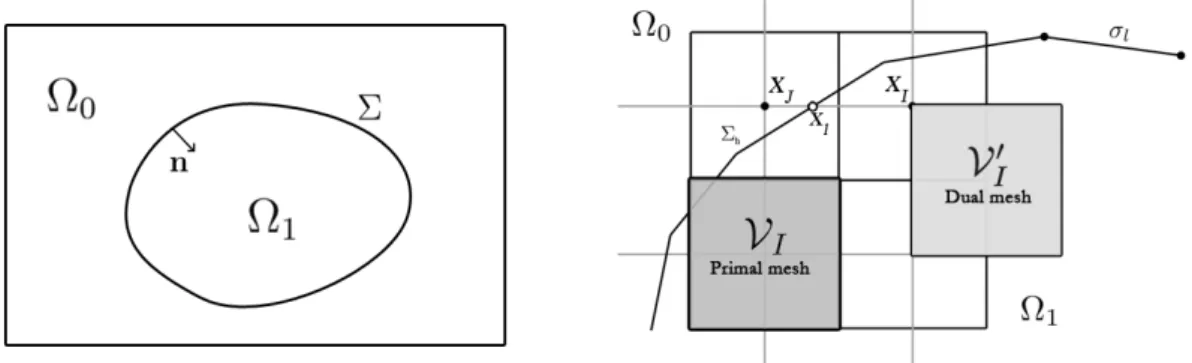
Let us consider the original domain of interest denoted by Ω0, typically the fluid domain, which is embedded inside
a simple computational domain Ω⊂ Rd. The auxiliary domain Ω
1, typically a solid particle or an obstacle, is then
such that Ω = Ω0∪ Σ ∪ Ω1where Σ is an immersed interface (see Fig. 1 left). Let n be the unit outward normal
vector to Ω0on Σ. Our objective is to numerically impose the adequate boundary or interface conditions on the
interface Σ. The continuous L2-penalty method for the incompressible Navier-Stokes equations consists in adding a term χε(u− uD) into the momentum equation
ρ ( ∂u ∂t + (u· ∇)u ) =−∇p + ρg + ∇ · [µ(∇u + ∇Tu)] +χ ε(u− uD) (15)
where 0 < ε≪ 1 denotes the penalty parameter and χ is the Heaviside function such as
χ(x) =
{
1 if x∈ Ω1 0 if x∈ Ω0.
In Ω0, the penalty term vanishes and the original momentum equation is retrieved. In Ω1, the equation tends to
3.2
Discretization
For the sake of simplicity the method is described in 2D for a scalar equation. The computational domain Ω is approximated with a curvilinear mesh Thcomposed of N× M (×L in 3D) cell-centered finite volumes (VI) for
I ∈ E, E being the set of index of the Eulerian orthogonal curvilinear structured mesh. Let xI be the vector
coordinates of the center of each volumeVI. The local characteristic space step hI of the volumeVI is defined
as the maximum length ofVI in each direction, whereas h denotes the Eulerian mesh step: h = supI∈EhI. This
grid is used to discretize the conservation equations. A dual grid is introduced for the management of the penalty method (in finite-difference discretization, the primal mesh is used). The grid lines of this dual cell-vertex mesh are defined by the network of the cell centers xI. The volumes of the dual mesh are denoted by (KI). The Eulerian
unknowns are noted ϕI which are the approximated values of ϕ(xI), i.e. the solution at the cell centers xI.
The discrete interface Σh, hereafter called the Lagrangian mesh, is given by a discretization of the original
inter-face Σ. It is described by a piecewise linear approximation of Σ: Σh={σl∈ Pd1−1, l∈ Lf}, K being the cardinal
ofLf andLf being the set of index of the Lagrangian mesh. Typically, σl are segments in 2D and triangles in
3D. The vertices of each face σlare denoted by xl,ifor i = 1, d and the set of all vertices is : {xl, l∈ Lv}. The
intersection points between the grid lines of the Eulerian dual mesh and the faces σlof the Lagrangian mesh are
denoted by{xi, i∈ I} (see Fig. 1 right).
The cell centers xI are sorted according to their location inside Ω0 or Ω1 with the discrete Heaviside function χI = χ(xI). This function is computed from Σhwith a Thread Ray-casting method [SVC10]. The principle is
to cast a ray from each Eulerian nodes. If the number of intersections between Σhand the ray is odd, the node is
inside the object, otherwise outside. The algorithm needs LM N K/ max(L, M, N ) intersection tests and is faster than the classical Ray-casting method [OSF05] which requires LM N K intersection tests. New sets of Eulerian points xI are defined near the interface such as one neighbor xJ verifying χJ ̸= χI exists, i. e. the segment
[xI; xJ] is cut by Σh. These Eulerian "interface" points are also sorted according to their location inside Ω0or Ω1.
Two sets{xI, I ∈ N0} and {xI, I ∈ N1} are so obtained, where N0 ={I, xI ∈ Ω0,∃ neighb(xI)∈ Ω1} and
N1={I, xI ∈ Ω1,∃ neighb(xI)∈ Ω0}.
The spatial order of the L2-penalty method directly depends on the discretization of χε(ϕ− ϕD). The VPM
[Ang89] discretizes the term for a node ϕias χεi(ϕi− ϕD) with ϕDthe boundary value at the vicinity of xi. As
the solution is considered as constant in each penalized cells, the shape of the immersed boundary is perceived by the fluid as being stair-stepped, or rasterized. This inaccurate description of the interface implies a first-order of spatial convergence [Ram07].
To reach a second-order of spatial accuracy, the sub-mesh penalty method (SMPM) [SVCA08, SVAC08] dis-cretizes the penalty term with χi
ε(Πiϕ− ϕD(xl)) where Πiis a polynomial interpolator.
We consider a point xI with I ∈ N1 and only one neighbor xJ in Ω0. The Lagrangian point xlis the
inter-section between [xI; xJ] and Σh(Fig. 1 right). The solution ϕ = ϕlhas to be satisfied at xlwhich implies in a
discrete point of view ΠIϕ(xl) = ϕD(xl) with Π theP11-interpolator (one-dimensional linear polynomial) between
the Eulerian unknowns uI and uJ:
ϕl= αIϕI+ αJϕJwith 0 < αI, αJ< 1 and αI+ αJ= 1 (16)
The coefficients αI and αJ are determined such as ΠIϕ(xI) = ϕI and ΠIϕ(xJ) = ϕJ. If now xI has a second
neighbor xKin Ω0, the intersection xmbetween [xI; xK] and Σhis considered. We choose xp, a new point of Σh
between xland xm(see Fig. 1 left). Practically, the barycenter between xmand xlis used. The resulting point xp
is not necessarily on Σhbut it does not spoil the second-order precision of the method since the distance d(xp, Σh)
between xp and Σh is varying likeO(h2). The solution ϕp(xp) is then approximated using aP21-interpolation
(two-dimensional linear polynomial)of the values ϕI, ϕJand ϕK:
ϕp= αIϕI + αJϕJ+ αKϕK, 0 < αI, αJ, αK < 1 , αI+ αJ+ αK= 1 (17)
We can also use aQ2
1-interpolation of ϕI, ϕJ, ϕKand ϕL, by extending the interpolation stencil with the point xL
which is the fourth point of the cell of the dual mesh defined by xI, xJand xK(see Fig. 1.right).
If Σhis regular enough, xI has almost never a third neighbor in Ω0. However, if it is the case, the first-order L2-penalty term χI
ε(ϕI− ϕD(xl)) is used. In any case, by decreasing the Eulerian mesh step h, we also decrease
the number of points xIhaving more than two neighbors in Ω0.
It has to be noticed that the penalty term is only required for nodes xI with I ∈ N1, i.e. for the nodes in Ω1with
of secondary interest (practically, the parts of the discretization matrix corresponding to these nodes are removed before the resolution of the liner system).
Concerning the application of the method to a Curvilinear grid, the computational domain can be "unfold" into a Cartesian domain where most of the computations are performed. Hence, the penalty constraints are build from the Cartesian grid with the standard Cartesian routines. The curvilinear to Cartesian projection is described in [SVC10] .
4
Penalty correction for the pressure correction methods
4.1
First-order correction
For a first-order penalty term, such a correction is easy to performed [PAC08]. Let us now write the momentum Navier-Stokes equation with a first-order penalty term :
ρ∂u
∂t = +RHS− ∇p + χ
ε(u− uD) (18)
In the standard method, (4)−(5) is considered to obtain the equation (6). The same operation is performed with the penalty term and the equation (6) becomes:
ρ ( un+1− u∗ ∆t ) =−∇p′+χ ε(u n+1− u∗) (19)
and the equation (7) becomes:
∇ · u∗=∇ · (∆t
ρ − χ ε)
−1∇p′. (20)
The velocity is then updated using (19) :
un+1= u∗− (∆t
ρ − χ ε)
−1∇p′. (21)
It is important to notice that the correction terms due to the fictitious domain method appears naturally with this walkthrough. The standard pressure update is not modified.
Remark 4.1 A classical problem with the elliptic equation (20) in the penalized approach is that the diffusion
coefficient varies in O(ε−1) in Ω1. Hence, a strong imposition of the penalty constraint produces a very high diffusion coefficient which leads to numerical instabilities. In [BF10], with the assumption that ρ is constant over the domain, the authors propose the following correction to avoid numerical instabilities :
ρ ∆t∇ · u ∗=∇ · ε ε + χ∇p n+1+1 ε(p n+1− p0) (22)
where p0is a prescribed pressure. The last term produces a L2-penalization of the pressure equation.
Remark 4.2 In [BF10], authors use the non-incremental version of the scheme and a first-order correction for
the pressure equation. However, the boundary condition is explicitly chosen as being the linear extrapolation of the solution and a second-order of spatial convergence is reached for a stationary case. In our approach, all the terms due to the penalization are of second-order and implicit.
4.2
Higher-order correction
A fully implicit second-order correction is now proposed. A consistant correction following the precedent walk-through with a penalty term of higher order is much more delicate. The first-order termχi
ε(ui−uD(xl)) is replaced
by χi
ε(Πiu− uD(xl)) with Πiu =
∑
j/xj∈Neighb(xi)
αjuj. The pressure equation (20) becomes, for each node xi:
∇ · u∗ i =∇ · ( ρ ∆t− χi εΠi) −1∇p′ (23)
which requires the calculation of the matrix corresponding to (∆tρ −χi
εΠi)−1before the resolution of the initial
system. A more simple method is chosen here even if it would be interesting to evaluate this first method. We start back with the equation (6) with a penalty term by following the natural walkthrough of the first-order correction :
un+1i − u∗i =−∆t ρ ∇p ′+∆tχi ρε Πi ( un+1− u∗) (24) developed as (1−∆tχi ρε Πi)(u ∗− un+1) = ∆t ρ ∇p ′. (25)
The key of this construction is to introduce Π′i, a new interpolator such as: Π′iu =
∑
j/xj∈Neighb(xi),i̸=j
αjuj. (26)
Hence, Πiu = αiui+ Π′iu and we have
( 1−∆tχi ρε (αi+ Π ′ i) ) (u∗− un+1) =∆t ρ ∇p ′. (27)
By construction, the nodes involved by Π′i are always in Ω0 where χ = 0 so the original pressure-correction
method occurs. Hence, using (9) we have ( 1−∆tχiαi ρε ) (u∗i − un+1i )− ( ∆tχi ρε Π ′ i ∆t ρ ∇p ′)=∆t ρ ∇p ′ (28) and we obtain un+1i = u∗i − ( ∆tχi ρε− ∆tχiαi Π′i∆t ρ ∇p ′+ ∆tεi ρε− ∆tχiαi ∇p′ ) . (29)
the equation of the velocity update. Using the divergence of (29) and∇ · un+1i = 0 we obtain the final correction equation ∇ · u∗ i =∇ · ( ∆tχi ρε− ∆tχiαi Π′i∆t ρ ∇p ′+ ∆tεi ρε− ∆tχiαi∇p ′). (30)
The parameter ε≪ 1 and we obtain at the limit : ∆tχi ρε− ∆tχiαi −→ 0 and ∆tε ρε− ∆tχiαi −→ ∆t ρ in Ω0when ε−→ 0 (31) as χ(xi) = 0 for xi∈ Ω0and ∆tχi ρε− ∆tχiαi −→ − 1 αi and ∆tε ρε− ∆tχiαi −→ 0 in Ω1 when ε−→ 0. (32) The pressure update is still pn+1 = pn + p′(−µ∇ · u∗). Using (24) to build the velocity update, the standard
equation (9) is recovered in Ω0.
A major advantage of this formulation is that the diffusion coefficient in the pressure equation (30) has generally an absolute value of magnitude ∆t/ρ which avoid the numerical instability of the first-order method. Critical values appears when the interface is very close to the penalized node or a neighbor of the penalized node. If we consider the case where a node xI ∈ Ω1has one neighbor xJ ∈ Ω0, the penalty constraint is αIuI+ (1−αI)uJ = uD(xl),
and here Π′Iu = (1− αI)uJ. Hence, the diffusion coefficient is (αI− 1)∆t/(αIρ) and is critical if the interface
Σhis close to the penalized node. In this case the coefficient is very small and the same problem as with the
first-order correction occurs. However we noticed that a correct solution can be obtained with a diffusion coefficient of magnitude 10−10. If the interface position leads to a smaller value, one can slightly move the interface to decrease
αI. The case αI ≪ 1 provides a large diffusion coefficient and produces a H1-penalty term [ABF99], that is to
4.3
Comparison to the Hikeno-Kajishima correction
This approach has been proposed by [IK07] for a DF-IBM method and is presented here for our interpolator Π. They propose the following velocity update
un+1i = u∗i − ( (1− χi) ∆t ρ ∇p ′− χ i Π′i∆tρ ∇p′ αi ) (33)
which is directly introduced and not obtained from the solved momentum equation (the consistency of the method is demonstrated afterwards). In our formulation, all the method is derived from the original momentum equation and the prediction equation so the consistency is naturally deduced. From (33) and the incompressibility constraint, the following equation is obtained :
∇ · u∗ i =∇ · ( (1− χi) ∆t ρ ∇p ′− χ i Π′i∆t ρ ∇p′ αi ) . (34)
and the pressure is updated as in the standard method
pn+1= p′+ pn. (35)
The method is applied too to the non-incremental fractional step method.
As can be seen, the equations obtained are different than with the present approach. Obviously, it is due to the way the boundary condition is imposed (penalty term with a coefficient 1/ε of dominant magnitude in our case or IBM direct-forcing term with Dirac function in [IK07]). However, the final pressure correction equation with the penalized correction (30) tends to (34) when ε tends to zero. The same result is obtained with the corresponding velocity updates.
Remark 4.3 For this correction (and the penalty correction presented here when ε → 0), the velocity in Ω1 is updated as un+1i = u∗i +Π ′ i ∆t ρ ∇p′ αi (36)
By construction of the interpolator Πiu = αiui+ Π′iu, no node of Ω1is involved in Π′i. Hence, as the pressure
correction in Ω0is
un+1i = u∗i −∆t
ρ ∇p
′, (37)
one can replace ∆t ρ ∇p ′by (u∗ i − u n+1 i ) to obtain un+1i = u∗i − Π′i(u∗i − un+1i ) αi . (38)
Considering the initial interpolator Πi, we obtain
Πiun+1i = Πiu∗i (39)
and the boundary constraint obtained in the predictor step is conserved. It induces as well that Πiu′i = 0. The
update of the velocity near the velocity is not necessarily null contrary to the linear combination of these velocities.
4.4
Temporal accuracy for the incremental pressure-correction
We study here the temporal accuracy of the pressure for the penalized incremental pressure-correction method with a first-order Euler scheme. The temporal accuracy for the base method is O(∆t) [GMS06]. The ideal equation system to solve is: [
A G D 0 ] [ un+1 pn+1 ] = [ r 0 ] (40)
with G the gradient operator, D the divergence operator, A the following sub-matrix
A = { ρ ∆t+ N− V − χ εΠ } (41)
with N the linearized discretization of the inertial term and V the discretization of the viscous term. The second member r is defined as ri= ∆t ρ u ∗ i − χi ε Πiu ∗. (42)
The velocity update (29) allows to write [ I BG 0 I ] [ un+1 pn+1 ] = [ u∗ pn+1 ] (43)
with I the identity matrix and B the matrix such as
B = { ∆tχi ρε− ∆tχiαi Π′i∆t ρ + ∆tε ρε− ∆tχiαi } . (44)
At last, the pressure elliptic equation yields [ A 0 D −DBG ] [ u∗ pn+1 ] = [ r 0 ] . (45)
As first noticed by Perot [Per93], the two systems (43) and (45) are a block LU decomposition of the system [ A ABG D 0 ] [ un+1 pn+1 ] = [ r 0 ] (46)
which allows us to write the error of the scheme using (40) :
AB = {( ρ ∆t+ N− V − χ εΠ ) ( ∆tχ ρε− ∆tχαΠ ′∆t ρ + ∆tε ρε− ∆tχα )} . (47)
We study the error in Ω0. We consider the matrices N0, N1, V0and V1such as V = V0+ V1and N = N0+ N1.
The matrice N0is such that{N0}i,j = {N}i,j if xj ∈ Ω0, else{N0}i,j = 0. The same occurs for V0. It is
necessary to split these contributions as the value of χ varies in B. Hence, we have
AB = {( ρ ∆t+ N0− V0 )∆t ρ + (N1− V1) ( ∆t ρε− ∆tαΠ ′∆t ρ + ∆tε ρε− ∆tα )} (48)
which tends to term in{1 + O(∆t)} when ε tends to zero. The first order is retrieved. We consider now the error in Ω1: AB = {(N0− V0−1εΠ′ )∆t ρ + ( ρ ∆t+ N1− V1− 1 εα ) ( ∆t ρε−∆tαΠ′ ∆tρ + ∆tε ρε−∆tα )} = {(N0− V0)∆t ρ + ( −1 ε+ ρ ρε−∆tα− ∆tα ε(ρε−∆tα) ) Π′ ∆tρ +(N1− V1) ( ∆t ρε−∆tαΠ′ ∆tρ + ∆tε ρε−∆tα ) +ρε−∆tαρε −ρε∆tα−∆tα} = { (N0− V0)∆tρ + (N1− V1) ( ∆t ρε−∆tαΠ′ ∆tρ + ∆tε ρε−∆tα ) + 1 } (49)
which also tends to a term in {1 + O(∆t)} when ε tends to zero. Hence, the order of the original method is retrieved. The same result with a quite similar analysis is obtained by [IK07].
4.5
Value of the penalty parameter
The value of the penalty parameter ε has an influence on the solution as the solution u∗obtained with the momen-tum equations converges toward the desired solution for the L2-norm with an order6 3/4 in ε [ABF99].
For the first-order method, the value of the parameter is more critical. In the present approach, the empirical value ε ≈ 10−10 is used. This value can varies depending on the linear solver. Nonetheless, taking ε≈ 10−20 in (21) will ensure the desired velocity inside the obstacle. For the second-order correction, ε can be taken suffi-ciently small to ensure Πu∗ = uDat machine accuracy when the high-order penalty term is used. The converged
5
Numerical experiments
The performances of the modified pressure-correction are evaluated here. The method is compared to the aug-mented Lagrangian method which does not require a correction. It is also an opportunity to compare the approaches in a more general point of view. When no analytical solution is available, a Richardson extrapolation is used to compute a reference solution [Roa98]. We consider three values h1, h2and h3of a numerical parameter verifying
consecutive ratios of two. The convergence rate θ and the reference solution fextare given by:
θ = ln (f h1−fh2 fh2−fh3 ) ln ( h1 h2 ) (50) fext= ( h2 h3 )θ fh3− fh2 ( h2 h3 )θ − 1 (51)
The asymptotical convergence zone has to be reached to obtain a relevant extrapolation.
5.1
Cylindrical Couette flow
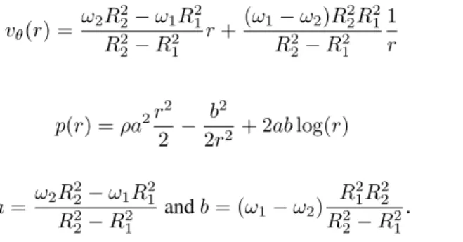
We consider a Couette flow between two cylinders of radius R1 = 0.5m and R2= 3m. Their angular velocities
are ω1= 0 rad.s−1and ω2= 2 rad.s−1. The solution is vθ(r) = ω2R22− ω1R21 R2 2− R21 r +(ω1− ω2)R 2 2R12 R2 2− R21 1 r (52)
for the velocity and
p(r) = ρa2r 2
2 −
b2
2r2 + 2ab log(r) (53)
for the pressure with
a =ω2R 2 2− ω1R21 R2 2− R21 and b = (ω1− ω2) R2 1R22 R2 2− R21 .
The NS equations are solved in a domain Ω = [−2 ; 2 + 0.1√2 ]× [ −2 ; 2 + 0.2√2 ]. The analytical solution is imposed on ∂Ω. The SMP method is used to impose a Dirichlet BC on the inner circle. For the augmented Lagrangian method, a value of the parameter dr = 10 is chosen.
Mesh L2rel. error. u Order L2rel. error. p Order
16 3.409× 10⁻³ 5.898× 10⁻³ 32 4.708× 10⁻⁴ 2.86 4.222× 10⁻³ 0.48 64 1.307× 10⁻⁴ 1.85 1.269× 10⁻³ 1.73 128 3.314× 10⁻⁵ 1.98 3.979× 10⁻⁴ 1.67 256 8.032× 10⁻⁶ 2.04 1.339× 10⁻⁴ 1.57 512 2.111× 10⁻⁶ 1.93 5.040× 10⁻⁵ 1.41 1024 5.281× 10⁻⁷ 2.00 2.040× 10⁻⁵ 1.30
Table 1: L2 relative errors in space and corresponding orders for the velocity and the pressure - augmented La-grangian an incremental pressure-correction methods
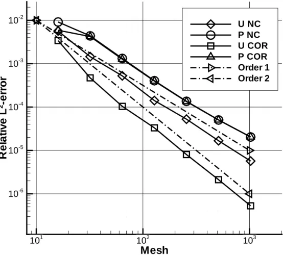
The convergence study of the L2relative spatial error is given in table 1 and plotted in figure 2. These results are obtained with the AL method. Similar results are obtained with the rotational pressure-correction with a negligible differential on the L2error demonstrating the spatial accuracy of the modification. As expected for such a case
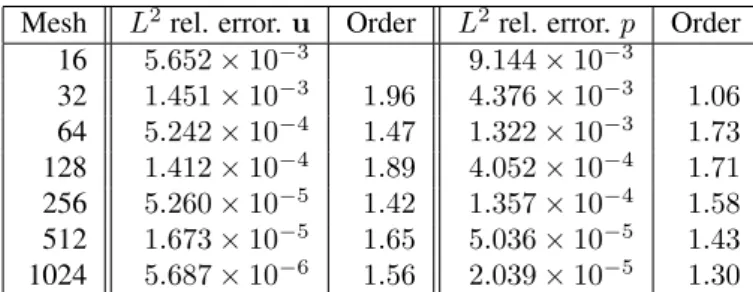
[SVCA08], a second order is obtain for the velocity. The convergence rate for the pressure error is around 1.5. The table 2 gives the same convergence study for the rotational method without immersed-boundary correction for a time step ∆t = 1s. As can be seen in figure 2, the lack of correction has almost no influence on the pressure. The convergence rate for the velocity is lower but acceptable. A factor ten is obtained between the solution with and without the correction for the finest mesh.
Mesh L2rel. error. u Order L2rel. error. p Order 16 5.652× 10⁻³ 9.144× 10⁻³ 32 1.451× 10⁻³ 1.96 4.376× 10⁻³ 1.06 64 5.242× 10⁻⁴ 1.47 1.322× 10⁻³ 1.73 128 1.412× 10⁻⁴ 1.89 4.052× 10⁻⁴ 1.71 256 5.260× 10⁻⁵ 1.42 1.357× 10⁻⁴ 1.58 512 1.673× 10⁻⁵ 1.65 5.036× 10⁻⁵ 1.43 1024 5.687× 10⁻⁶ 1.56 2.039× 10⁻⁵ 1.30
Table 2: L2 relative errors in space and corresponding orders for the velocity and the pressure -Timmermans
method without immersed boundary correction
The time evolution of the solution is now evaluated. For a case with Dirichlet boundary conditions, [GSLF05, GMS06] give for the rotational method a rate of O(∆t2) for the velocity and O(∆t3
2) for the pressure.
Simulations with a 64× 64 mesh are conducted with different time steps and velocity-pressure coupling meth-ods. The instant Tp when the L2error on the pressure reaches 1.5× 10⁻³and the instant Tv when the L2 error
on the velocity reaches 1.5× 10⁻⁴are considered to study the convergence. The table 4 shows the convergence of these values for the augmented Lagrangian and rotational pressure-correction methods, and for the Euler tem-poral schemes. The reference values are computed with the Richardson extrapolation using the three more refined values. A clear first order of convergence is obtained for the velocity and the pressure for both velocity-pressure coupling methods. Except for the larger time-steps, both methods gives the same results.
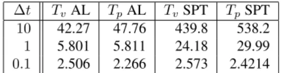
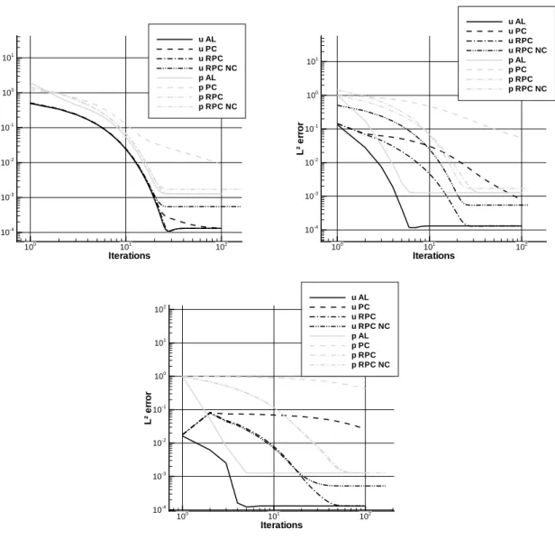
The figure 3 shows the evolution of the spatial error with respect to the number of time iterations for ∆t = 0.1s, ∆t = 1s and ∆t = 10s while the table 3 gives the values of Tvand Tpfor these time steps. Due to its strong
implicitation, the AL method is always converged faster than the pressure-corrections. One can notice that the temporal evolution of the solution for the rotational method without correction is quite similar to the evolution of the corrected methods up to an error of 10−3on the velocity. For this case, the interest of the correction seems to be minor. The figure 3 shows that the convergence of the incremental pressure-correction is much slower than with the other methods. For the present case, reaching the same level of error than with the two others methods is prohibitive.
The curves of convergence for the second-order Gear scheme are show in figure 4 (the error convergence for the velocity with the augmented Lagrangian method and for the first-order temporal scheme is given for comparison). The values are given in table 5. An irregular convergence is observed for the velocity. For time steps inferior to 0.01s, the error is under the error for the Euler scheme for all values and the asymptotical convergence zone seems to be reached. A first-order of convergence rate is obtained for the pressure. An order of about 0.8 is obtained for the velocity with the pressure-correction which is far from the theoretical order of 2. The augmented Lagrangian method has lower errors but its convergence rate is about 0.5 in the asymptotical zone. Studies conducted in [FLPA09] suggest that the augmented Lagrangian should reach a first-order for the velocity and the pressure. The same behavior is obtained in [AJL]. As the convergence rates are better for the first-order temporal scheme, a saturation effect can be involved. Compared to the classical studies, we have the immersed boundary correction here which could cause this saturation. The value of the parameter ε is not involved here as the converged equations in ε gives the same results. In this case the theoretical error study suggests a first-order of convergence for the pressure. The use of a relatively coarse mesh seems not to be involved as we use the Richardson extrapolation to compute the solution so one can suppose that the spatial error does not mix with the temporal error. This point has to be investigated further. The figure 4 shows the convergence for the augmented Lagrangian method with
dr = 100. The error on the pressure is close to the other methods. For the smallest time steps, the error on the
velocity oscillates around a value so we cannot use the Richardson extrapolation. This values is different from the value obtained with the other methods, so another saturation effect seems to be involved. For this reason, the reference value of the pressure-correction and the augmented Lagrangian with dr = 10 is taken. Even if the convergence is stopped for the smaller time steps, an excellent error (compared to the other methods) is obtained.
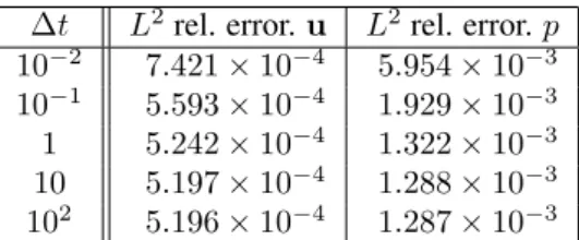
To finish with this case, the table 6 shows the spatial errors for various time steps with the rotational method without correction. Contrary to the corrected methods, the error at the stationary state depends on the time step even if its influence is small here. A quite surprising results is that the error decreases when the time step increases while Domenichini [Dom08] has noticed the contrary (but for different cases and with a spectral solver).
∆t TvAL TpAL TvSPT TpSPT
10 42.27 47.76 439.8 538.2 1 5.801 5.811 24.18 29.99 0.1 2.506 2.266 2.573 2.4214
Table 3: Temporal convergence of the error on the velocity and the pressure for the augmented Lagrangian and the rotational methods for large time steps for the Couette flow
∆t TuAL Order TpAL Order TuSPT Order TpSPT Order
Ref 2.107 1.863 2.107 1.863 128× 10−3 5.168× 10⁻¹ 5.172× 10⁻¹ 6.402× 10⁻¹ 1.034× 10+0 64× 10−3 2.591× 10⁻¹ 1.00 2.584× 10⁻¹ 1.00 2.835× 10⁻¹ 1.18 2.968× 10⁻¹ 1.80 32× 10−3 1.315× 10⁻¹ 0.98 1.304× 10⁻¹ 0.99 1.353× 10⁻¹ 1.07 1.381× 10⁻¹ 1.10 16× 10−3 6.630× 10⁻² 0.99 6.539× 10⁻² 1.00 6.651× 10⁻² 1.02 6.654× 10⁻² 1.05 8× 10⁻³ 3.328× 10⁻² 0.99 3.268× 10⁻² 1.00 3.299× 10⁻² 1.01 3.259× 10⁻² 1.03 4× 10⁻³ 1.665× 10⁻² 1.00 1.636× 10⁻² 1.00 1.640× 10⁻² 1.01 1.614× 10⁻² 1.01 2× 10⁻³ 8.339× 10⁻³ 1.00 8.185× 10⁻³ 1.00 8.182× 10⁻³ 1.00 8.019× 10⁻³ 1.01 1× 10⁻³ 4.177× 10⁻³ 1.00 4.096× 10⁻³ 1.00 4.082× 10⁻³ 1.00 3.984× 10⁻³ 1.01 Table 4: Temporal convergence of the error on the velocity and the pressure for the augmented Lagrangian and the rotational methods - Gear 1 scheme for the Couette flow
∆t TuAL Order TpAL Order TuSPT Order TpSPT Order
Ref 2.107 1.863 2.107 1.863 128× 10−3 1.918× 10⁻¹ 8.743× 10⁻¹ 3.852× 10⁻² 6.724× 10⁻¹ 64× 10−3 2.531× 10⁻² 2.92 4.095× 10⁻² 4.42 6.041× 10⁻³ 2.67 3.887× 10⁻² 4.11 32× 10−3 3.569× 10⁻³ 2.83 2.356× 10⁻² 0.80 1.157× 10⁻³ 2.38 1.846× 10⁻² 1.07 16× 10−3 2.769× 10⁻⁴ 3.69 1.290× 10⁻² 0.87 1.802× 10⁻³ -0.64 9.048× 10⁻³ 1.03 8× 10⁻³ 6.918× 10⁻⁴ -1.32 6.687× 10⁻³ 0.95 1.251× 10⁻³ 0.53 4.632× 10⁻³ 0.97 4× 10⁻³ 5.336× 10⁻⁴ 0.37 3.428× 10⁻³ 0.96 7.212× 10⁻⁴ 0.80 2.326× 10⁻³ 0.99 2× 10⁻³ 3.756× 10⁻⁴ 0.51 1.753× 10⁻³ 0.97 4.120× 10⁻⁴ 0.81 1.168× 10⁻³ 0.99 1× 10⁻³ 2.645× 10⁻⁴ 0.51 8.976× 10⁻⁴ 0.97 2.357× 10⁻⁴ 0.81 5.862× 10⁻⁴ 0.99 Table 5: Temporal convergence of the error on the velocity and the pressure for the augmented Lagrangian and the rotational methods - Gear 2 scheme for the Couette flow
∆t L2rel. error. u L2rel. error. p 10−2 7.421× 10⁻⁴ 5.954× 10⁻³ 10−1 5.593× 10⁻⁴ 1.929× 10⁻³ 1 5.242× 10⁻⁴ 1.322× 10⁻³ 10 5.197× 10⁻⁴ 1.288× 10⁻³ 102 5.196× 10⁻⁴ 1.287× 10⁻³
Table 6: L2relative errors in space for the non-corrected rotational method for various time steps for the Couette
flow
∆t/∆tmin Period/∆tmin(RPC) Order Period/∆tmin(AL) Order
Ref 4.667× 10² 4.694× 10² 128 1.137× 10³ 1.043× 10³ 64 7.973× 10² 1.02 7.506× 10² 1.02 32 6.282× 10² 1.03 6.241× 10² 0.86 16 5.493× 10² 0.96 5.530× 10² 0.88 8 5.107× 10² 0.90 5.134× 10² 0.92 4 4.896× 10² 0.94 4.920× 10² 0.96 2 4.785× 10² 0.96 4.806× 10² 1.00 1 4.726× 10² 0.96 4.750× 10² 1.00
Table 7: Period of the oscillations with the rotational pressure correction (RPC) and the augmented Lagrangian (AL) with a Gear 1 temporal scheme for the flow past a cylinder at Re = 100
5.2
Flow past a cylinder
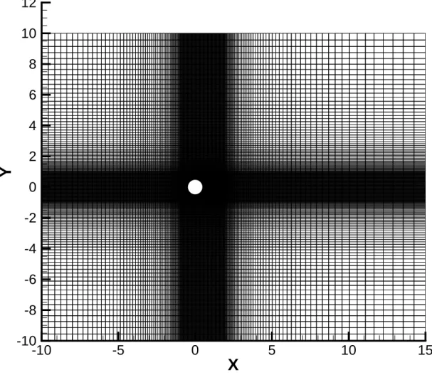
The instationary flow past a cylinder of unit diameter is now simulated to study the temporal order of the method for an instationary case. We consider a cylinder of diameter D in a domain Ω = [−10R ; 15R ]×[ −10R ; 10R ]. The inlet velocity V and the fluid properties are set such as the Reynolds number is equal to 100. The computational mesh is composed of 175× 150 cells with an inner zone of dimensions [ −D ; 2D ] × [ −D ; D ] with a constant space step covered by 75× 50 cells. The figure 6 shows the mesh and the position of the cylinder. An Orlanski open boundary condition [Orl76] is imposed for the outflow.
The vorticity and the pressure are shown in figure (5). On can see that the vorticity in the periodic Bénard-von Kármán vortex street is strongly decaying with the X direction compared to the standard solution of the litteraure. This difference is due to the coarseness of the mesh. However, the aim here is not to compare our results with the literacy so the size of the computational mesh is relatively moderate.
The table 8 gives the values of a period of oscillation (adimentionalised by the minimum time step) for different time steps with the augmented Lagragian an rotational methods with the first and second-order Gear schemes for the time derivatives. The convergence order is determined with the Richardson extrapolation performed with the three more refined time steps. The results in term of relative error are given in figure 7.
For both time schemes, the differences between AL and the rotational methods are non-negligible for the larger
∆t/∆tmin Period/∆tmin(RPC) Order Period/∆tmin(AL) Order
Ref 4.673× 10² 4.691× 10² 128 1.083× 10³ 1.016× 10³ 64 7.386× 10² 1.18 7.278× 10² 1.08 32 5.671× 10² 1.44 5.762× 10² 1.27 16 5.051× 10² 1.40 5.102× 10² 1.39 8 4.832× 10² 1.25 4.853× 10² 1.36 4 4.740× 10² 1.23 4.760× 10² 1.27 2 4.701× 10² 1.18 4.722× 10² 1.21 1 4.685× 10² 1.18 4.706× 10² 1.21
Table 8: Period of the oscillations with the rotational pressure correction (RPC) and the augmented Lagrangian (AL) with a Gear 2 temporal scheme for the flow past a cylinder at Re = 100
time steps, with a greater accuracy for the AL. As for the precedent case, it shows the advantage of the AL to deal with larger time steps. For the other time steps, both methodology reach an almost similar accuracy. For the smaller time steps (where the asymptotic convergence seems to be reached) the convergence orders on the velocity and the pressure is about 1 for the Euler scheme and about 1.2 for the second-order Gear scheme. From [GSLF05], the rate of error for the L2-norm of the velocity of O(∆t3
2) is expected.
6
Conclusion
The correction of the first-order L2-penalty method for the pressure-correction methods has been extended to a second-order with the Sub-mesh penalty method. The correction converges toward the Hikeno and Kajishima [IK07] correction which is designed for a direct-forcing IBM method. The consistency of the method is directly deduced from its construction.
A brief theoretical analysis has proven that the temporal error of the pressure correction method with a first-order Gear scheme was not altered. Again, this point is similar to the Hikeno-Kajishima correction. A study with higher integration schemes is now desirable.
Numerical experiments have been carried out. The correction has been compared to the augmented Lagrangian method and the same results have been obtained in space for the cylindrical Couette flow. For this first case, conver-gence rates of 2 and 1.3 in the L2-error norm for the velocity and the pressure have been obtained. It corresponds
to the known performances of the rotational method with Dirichlet boundary conditions. Concerning the flow past a cylinder at Re = 100, the study has shown a maximum convergence order for both augmented Lagrangian and rotational methods of 1.20. Those results are close to the literature where a convergence rate between O(∆t) and
O(∆t32) is expected [GMS06]. A combination with the second-order open boundary conditions of [PGA11] could
be investigated.
As for a small enough penalty parameter ε the present methodology is equivalent to a corrected direct-forcing IBM, especially the method of [TF03], the conclusions of this study can be extended to this method.
This work is also a more general comparison between the rotational pressure-correction and the augmented Lagrangian methods (and this last method can a priori be applied to any DF-IBM method). The results show that the spatial accuracy is the same for both methods. Concerning the time accuracy, the AL approach seems to be more efficient with very-high time steps. For moderate and low time-steps, one cannot conclude. Almost no differences have been obtained with the case of the flow past a cylinder. For the Couette flow, quite similar results are obtained for the pressure. For the velocity, the results depends on the time step. For the smaller time steps, the convergence of the AL method decreases while the absolute temporal accuracy is still better than with the rotational method. It has been shown that the value of the penalty parameter dr had an influence on the convergence rate. The influence of the number of sub-iterations could be evaluated too. Increasing the number of sub-iteration generally enhances the convergency at the expense of the computational cost. All these considerations show the complexity of a comparative study between those methods (with and without immersed boundary modification). A future work devoted to an extended comparison would be of high interest, especially if simulations of multiphase flows are performed.
References
[ABF99] Philippe Angot, Charles-Henri Bruneau, and Pierre Fabrie. A penalization method to take into account obstacles in incompressible viscous flows. Numerische Mathematik, 81:497–520, 1999.
[AHU58] K. J. Arrow, L. Hurwicz, and H. Uzawa. Studies in linear and Nonlinear Programming - Iterative
method for concave programming. Stanford University Press, 1958.
[AJL] Ph. Angot, M. Jobelin, and J.-C. Latché. Error analysis of the penalty-projection method for the time-dependant stokes equations. International Journal on Finite Volumes, 6:1–26.
[Ang89] P. Angot. Contribution à l’étude des transferts thermiques dans des systèmes complexes aux
com-posants électroniques. PhD thesis, Université Bordeaux I, 1989.
[Arq84] E. Arquis. Convection mixte dans une couche poreuse verticale non confinée. Application à l’isolation perméodynamique. PhD thesis, Université Bordeaux I, 1984.
[BF10] Michel Belliard and Clarisse Fournier. Penalized direct forcing and projection schemes for navier-stokes. Comptes Rendus Mathematique, 348(19-20):1133 – 1136, 2010.
[CB99] J.P. Caltagirone and J. Breil. A vectorial projection method for solving the navier-stokes equations.
C. R. Acad. Sci. Paris, 327:1179 – 1184, 1999.
[Dom08] Federico Domenichini. On the consistency of the direct forcing method in the fractional step solution of the navier-stokes equations. Journal of Computational Physics, 227:6372–6384, 2008.
[FG82] M. Fortin and R. Glowinski. Méthodes de lagrangien augmenté. Application à la résolution numérique de problèmes aux limites. Dunod Paris, 1982.
[FLPA09] C. Févriére, J. Laminie, P. Poullet, and Ph. Angot. On the penalty-projection method for the navier-stokes equations with the mac mesh. Journal of Computational and Applied Mathematics, 226:228– 245, 2009.
[FVOMY00] E. A. Fadlun, R. Verzicco, P. Orlandi, and J. Mohd-Yusof. Combined immersed-boundary finite-difference methods for three-dimensional complex flow simulations. Journal of Computational
Physics, 161(1):35 – 60, 2000.
[GMS06] J.L. Guermond, P. Minev, and Jie Shen. An overview of projection methods for incompressible flows. Computer Methods in Applied Mechanics and Engineering, 195(44-47):6011 – 6045, 2006.
[God78] K. Goda. A multistep technique with implicit difference schemes for calculating two- or three-dimensional cavity flows. Journal of Computational Physics, 30:76 – 95, 1978.
[GPHJ99] R. Glowinski, T. W. Pan, T. I. Hesla, and D. D. Joseph. A distributed lagrange multiplier/fictitious domain method for particulate flows. International Journal of Multiphase Flow, 25(5):755 – 794, 1999.
[GSLF05] E. Guendelman, A. Selle, F. Losasso, and R. Fedkiw. Coupling water and smoke to thin deformable and rigid shells. In Proceedings of ACM SIGGRAPH 2005, pages 973–981, 2005.
[Gus78] I. Gustafsson. On First and Second Order Symmetric Factorization Methods for the Solution of
Ellip-tic Difference Equations. Research report, Department of Computer Sciences, ChalmersUniversity
of Technology and the University of Gateborg. la, 1978.
[IK07] T. Ikeno and T. Kajishima. Finite-difference immersed boundary method consistent with wall conditions for incompressible turbulent flow simulations. Journal of Computational Physics,
226(2):1485–1508, 2007.
[JC98] Hans Johansen and Phillip Colella. A cartesian grid embedded boundary method for poisson’s equation on irregular domains. Journal of Computational Physics, 147(1):60 – 85, 1998.
[KAPC00] Kodor Khadra, Philippe Angot, Sacha Parneix, and Jean-Paul Caltagirone. Fictitious domain ap-proach for numerical modelling of navier-stokes equations. International Journal for Numerical
Methods in Fluids, 34:651–684, 2000.
[KKC01] J. Kim, D. Kim, and H. Choi. An immersed boundary finite volume method for simulations of flow in complex geometries. Journal of Computational Physics, 171:132–150, 2001.
[MCJ01] Peter McCorquodale, Phillip Colella, and Hans Johansen. A cartesian grid embedded boundary method for the heat equation on irregular domains. Journal of Computational Physics, 173(2):620 – 635, 2001.
[MI05] Rajat Mittal and Gianluca Iaccarino. Immersed boundary methods. Annual Review in Fluid
Me-chanics, 37:239 – 261, 2005.
[Moh97] J. Mohd-Yusof. Combined immersed boundary/b-spline methods for simulations of flows in com-plex geometries. Technical report, NASA ARS/Stanford University CTR, 1997.
[Orl76] I. Orlanski. A simple boundary condition for unbounded hyperbolic flows. Journal of Computational
[OSF05] Carlos J. Ogayar, Rafael J. Segura, and Francisco R. Feito. Point in solid strategies. Computers &
Graphics, 29(4):616–624, 2005.
[PAC08] P. Fabrie P. Angot and J.-P. Caltagirone. Finite Volumes for Complex Applications V, chapter Vector Penalty-Projection Methods for the Solution of Unsteady Incompressible Flows, pages 169–176. Wiley, 2008.
[Per93] J. Blair Perot. An analysis of the fractional step method. Journal of Computational Physics,
108(1):51 – 58, 1993.
[Pes72] Charles S. Peskin. Flow patterns around heart valves: A numerical method. Journal of
Computa-tional Physics, 10(2):252–271, 1972.
[Pes02] Charles S. Peskin. The immersed boundary method. Acta Numerica, 11:479–517, 2002.
[PGA11] A. Poux, S. Glockner, and M. Azaïez. Improvements on open and traction boundary conditions for navier-stokes time-splitting methods. Journal of Computational Physics, 230(10):4011 – 4027, 2011.
[RAB07] Isabelle Ramière, Philippe Angot, and Michel Belliard. A general fictitious domain method with immersed jumps and multilevel nested structured meshes. Journal of Computational Physics,
225(2):1347–1387, 2007.
[Ram07] Isabelle Ramière. Convergence analysis of the q1-finite element method for elliptic problems
with non-boundary-fitted meshes. International Journal for Numerical Methods in Engineering, 75:1007–1052, 2007.
[Roa98] P. J. Roache. Verification and validation in computational science and engineering. Hermosa Pub-lishers, Albuquerque, 1998.
[Sar09] A. Sarthou. Fictitious domain methods for the elliptic and Navier-Stokes equations. Application
to fluid-structure coupling. PhD thesis, Université Bordeaux I, 2009. The document is mainly in
english.
[She92] J. Shen. On error estimates of some higher order projection and penalty-projection methods for navier-stokes equations. Numerische Mathematik, 62:49–73, 1992.
[SVAC08] A. Sarthou, S. Vincent, P. Angot, and J.-P. Caltagirone. Finite Volumes for Complex Applications V, chapter The sub-mesh-penalty method, pages 633–640. Wiley, 2008.
[SVC10] A. Sarthou, S. Vincent, and J.P. Caltagirone. A second-order curvilinear to cartesian transforma-tion of immersed interfaces and boundaries. applicatransforma-tion to fictitious domains and multiphase flows.
Computers & Fluids, In Press, Corrected Proof:–, 2010.
[SVCA08] A. Sarthou, S. Vincent, J.-P. Caltagirone, and P. Angot. Eulerian-Lagrangian grid coupling and penalty methods for the simulation of multiphase flows interacting with complex objects.
Interna-tional Journal for Numerical Methods in Fluids, 56(8):1093–1099, 2008.
[TC07] Kunihiko Taira and Tim Colonius. The immersed boundary method: A projection approach. Journal
of Computational Physics, 225:2118–2137, 2007.
[TF03] Yu-Heng Tseng and Joel H. Ferziger. A ghost-cell immersed boundary method for flow in complex geometry. Journal of Computational Physics, 192(2):593–623, December 2003.
[TMV96] L.J.P. Timmermans, P.D. Minev, and F.N. Van De Vosse. An approximate projection scheme for incompressible flow using spectral elements. International Journal of Numerical Methods in Fluid, 22:673–688, 1996.
[VCLR04] Stéphane Vincent, Jean-Paul Caltagirone, Pierre Lubin, and Tseheno Nirina Randrianarivelo. An adaptative augmented lagrangian method for three-dimensional multimaterial flows. Computers and
[VIFO01] R. Verzicco, G. Iaccarino, M. Fatica, and P. Orlandi. Flow in a impeller stirred tank using an immersed boundary method. Annual research brief, NASA Center for Turbulence Research, 2001.
[Vor92] H.A. Van Der Vorst. Bi-cgstab: a fast and smoothly converging variant of bi-cg for the solution of nonsymmetric linear systems. SIAM Journal on Scientific and Statistical Computing, 13(2):631– 644, 1992.
[VSC] Stéphane Vincent, Arthur Sarthou, Jean-Paul Caltagirone, Fabien Sonilhac, Pierre Février, Christian Mignot, and Grégoire Pianet. Augmented lagrangian and penalty methods for the simulation of two-phase flows interacting with moving solids. application to hydroplaning flows interacting with real tire tread patterns. Journal of Computational Physics, 230(4):956–983, 2010.
Mesh
R
e
la
ti
v
e
L
²-e
rr
o
r
10
110
210
310
-610
-510
-410
-310
-2U NC
P NC
U COR
P COR
Order 1
Order 2
Figure 2: Evolution of the spatial error for the velocity u and the pressure p with (COR) and without (NC) the correction for the Couette flow
Iterations L ² e rr o r 100 101 102 10-4 10-3 10-2 10-1 100 101 u AL u PC u RPC u RPC NC p AL p PC p RPC p RPC NC Iterations L ² e rr o r 100 101 102 10-4 10-3 10-2 10-1 100 101 u AL u PC u RPC u RPC NC p AL p PC p RPC p RPC NC Iterations L ² e rr o r 100 101 102 10-4 10-3 10-2 10-1 100 101 102 u AL u PC u RPC u RPC NC p AL p PC p RPC p RPC NC
Figure 3: Evolution of the L2-norm of the spatial error for ∆t = 0.1s, ∆t = 1s and ∆t = 10s for the Couette flow
for the augmented Lagrangian (AL), the incremental pressure-correction (PC), the rotational pressure-correction (RPC) and the not-corrected the rotational pressure-correction (RPC NC)