HAL Id: ird-00540604
https://hal.ird.fr/ird-00540604
Submitted on 29 Nov 2010
HAL is a multi-disciplinary open access archive for the deposit and dissemination of sci-entific research documents, whether they are pub-lished or not. The documents may come from teaching and research institutions in France or
L’archive ouverte pluridisciplinaire HAL, est destinée au dépôt et à la diffusion de documents scientifiques de niveau recherche, publiés ou non, émanant des établissements d’enseignement et de recherche français ou étrangers, des laboratoires
Estimate of the non-linear growth rate of yellowfin tuna
(Thunnus albacares) in the Atlantic and Indian oceans
from tagging data.
Daniel Gaertner, Emmanuel Chassot, Alain Fonteneau, Jean-Pierre Hallier,
Francis Marsac
To cite this version:
Daniel Gaertner, Emmanuel Chassot, Alain Fonteneau, Jean-Pierre Hallier, Francis Marsac. Estimate of the non-linear growth rate of yellowfin tuna (Thunnus albacares) in the Atlantic and Indian oceans from tagging data.. Collective Volume of Scientific Papers, ICCAT, 2010, 65 (2), pp.683-694. �ird-00540604�
SCRS/2009/042 Collect. Vol. Sci. Pap. ICCAT, 65(2): 683-694 (2010)
ESTIMATE OF THE NON-LINEAR GROWTH RATE OF
YELLOWFIN TUNA (THUNNUS ALBACARES) IN THE ATLANTIC
AND INDIAN OCEANS FROM TAGGING DATA
Daniel Gaertner1, Emmanuel Chassot1, Alain Fonteneau1,
Jean Pierre Hallier2 and Francis Marsac1
SUMMARY
In the lack of a satisfactory formulation for the two-stanza growth curve of yellowfin (Thunnus
albacares), estimates of growth rate by size class can be an alternative as an input for
integrated models. From tagging data collected in the Atlantic and Indian Oceans, we show however that for growth rate that does not follow a classical linear decreasing trend over size, simple estimates of length increments by size are biased due to an averaging effect of the time spent at liberty. We simulate length at recapture to illustrate the magnitude of the bias which can be expected depending on the duration of the time at liberty. Our results suggest that for large time at liberty growth rates by size are smoothed in such a way that the Von Bertalanffy model could erroneously be considered as a good alternative. With the aim of removing this bias we used a generalized additive model (GAM) to calculate an instantaneous growth rate by size (i.e., fixing time at liberty at 1 day at sea). The predicted growth rates by size are lower than the apparent growth rates but are similar in magnitude and in shape with observed growth rates for moderate times at liberty (< 90 days at sea). In the light of our findings, we suggest that hard part reading analyses, which in general reject the two-stanza growth assumption, could have been affected by the same type of bias.
RÉSUMÉ
Faute d’une formulation satisfaisante pour la courbe de croissance à deux stances de l’albacore (Thunnus albacares), les estimations du taux de croissance par classe de taille peuvent constituer une option alternative comme donnée d’entrée pour les modèles intégrés. A partir des données de marquage recueillies dans l’océan Atlantique et l’océan Indien, nous démontrons toutefois que pour le taux de croissance qui ne suit pas une tendance descendante linéaire classique des tailles, les simples estimations des augmentations de longueur par taille sont biaisées en raison de l’utilisation de valeurs moyennes du temps passé en liberté. Nous simulons la longueur à la récupération afin d’illustrer l’ampleur du biais qui peut être escompté en fonction de la durée du temps passé en liberté. Nos résultats suggèrent que pour un grand laps de temps en liberté, les taux de croissance par taille sont aplanis de telle façon que le modèle Von Bertalanffy pourrait erronément être considéré comme une bonne alternative. Dans le but de supprimer ce biais, nous avons utilisé un modèle additif généralisé (GAM) pour calculer un taux de croissance instantané par taille (c’est-à-dire établissant le temps passé en liberté à 1 journée en mer). Les taux de croissance par taille prédits sont plus faibles que les taux de croissance apparents, mais ils sont similaires en importance et en taille aux taux de croissance observés pour des périodes de temps modérées en liberté (< 90 jours en mer). A la lumière de nos conclusions, nous suggérons que les analyses de la lecture des structures osseuses, qui en général reflètent le postulat de croissance en deux stances, pourraient avoir été affectées par le même type de biais.
RESUMEN
A falta de una formulación satisfactoria para la curva de crecimiento de dos estanzas del rabil (Thunnus albacares), las estimaciones de la tasa de crecimiento por clase de talla pueden ser una alternativa como entrada para modelos integrados. A partir de datos de marcado recopilados en el Atlántico y en el Índico, demostramos sin embargo que, dado que la tasa de
1 UMR EME, Institut de Recherche pour le Développement (IRD), UR 109, Centre de Recherche Halieutique Méditerranéenne et Tropicale,
BP 171, 34203 Sète Cedex, France.
2 IRD and Regional Tuna Tagging Project–Indian Ocean (RTTP-IO), c/o Indian Ocean Tuna Commission (IOTC), PO Box 1011, Victoria,
Seychelles.
crecimiento no sigue una clásica tendencia descendente lineal a lo largo de la talla, las estimaciones simples de incrementos de longitud por talla están sesgadas debido a un efecto promediador del tiempo pasado en libertad. Simulamos la talla en el momento de la recaptura para ilustrar la magnitud del sesgo que puede esperarse dependiendo de la duración del tiempo en libertad. Nuestros resultados sugieren que para un gran tiempo en libertad, las tasas de crecimiento por talla se alisan de tal forma que el modelo de von Bertalanffy podría ser erróneamente considerado una buena alternativa. Con el objetivo de eliminar este sesgo, hemos utilizado un modelo aditivo generalizado (GAM) para calcular una tasa de crecimiento instantánea por talla (es decir, fijando el tiempo en libertad en 1 día en el mar). Las tasas de crecimiento por talla predichas son inferiores a las tasas aparentes de crecimiento pero son similares en magnitud y en forma a las tasas de crecimiento observadas para tiempos moderados en libertad (<90 días en el mar). Teniendo en cuenta nuestros hallazgos, sugerimos que los análisis de lectura de partes duras, que en general rechazan el supuesto de crecimiento de dos estanzas, podrían haberse visto afectados por el mismo tipo de sesgo.
KEYWORDS
Growth curves, tagging, simulation, yellowfin
1. Introduction
The individual growth of yellowfin tuna (Thunnus albacares) was initially modeled with the conventional Von Bertalanffy model (Yang et al, 1969, Le Guen and Sakagawa 1973). However, it was suggested in the early 1980s that a two-stanza growth model with a period of slow growth rates for young fish followed by a sudden increase in growth rate around 65-70 cm could be more appropriate (Fonteneau,1980). This nonconventional pattern in growth has been described later for yellowfin caught by different fisheries operating in other parts of the world ocean, based on different methods, such as length frequency analysis, hard part reading and tagging data analyses (Bard 1984, Wild, 1986, Marsac and Lablache 1985, Gaertner and Pagavino, 1991, Lehodey and Leroy, 1999). As an alternative of the classical Von Bertalanffy model, several models such as Gompertz and Richard’s curves (Bard, 1984; Wild, 1986, Bard et al. 1991), or a 5-parameters model (Gascuel et al. 1992) have been proposed. Nevertheless, with exceptions of Wild (1986) and Lehodey and Leroy (1999), several growth studies conducted from hard part analyses do not support the concept of the two-stanza growth model (Bayliff 1988; Lessa and Duarte-Neto 2004; Shuford et al. 2007). As a consequence, questions remain concerning the most appropriate growth model for yellowfin tuna.
In the lack of an appropriate growth model, Fonteneau and Gascuel (2008) suggested that instead of attempting to estimate the growth curve parameters within the framework of integrated models (e.g., Multifan-CL, etc), the direct implementation of observed growth rates by size class in such models might be a good alternative. This assertion is appealing but caution should be done on the values of the apparent growth rate obtained from tagging data. Indeed, a simple plot of growth rate by size class for different times at liberty for the Atlantic and the Indian Ocean yellowfin show changes in (1) the amplitude of growth rate by size and (2) the shape of the curve (Figure 1). It should be stressed that the linear decreasing trend in growth rate that characterizes the classical Von Bertalanffy model seems to be found only for large values of time at liberty.
The aim of this note is to show that the apparent non-linear growth rate at size obtained from tagging data cannot be used directly in integrated stock assessment model; i.e., without accounting for the bias due to the effect of time at liberty. This paper is constructed as follows: (i) we first compare the apparent growth rate over length at release obtained from tagging data in both oceans, (ii) from the 2 sets of tagging data, we perform an average pattern of apparent growth rate by size and we show by a simple simulation of length at recapture that depending on the value of time at liberty, the resulting growth rate by size may vary widely from a non-linear form to the conventional Von Bertalanffy decreasing linear form, (iii) based on a generalized additive modeling approach we propose a correction procedure to remove the effect of time at liberty on growth rate by size, (iv) to validate our approach, we finally compare (a) GAM predicted growth rates with observed growth rates for times at liberty shorter than 90 days at sea and (b) simulated lengths at recapture, resulting from the combination of predicted growth rates and observed times at liberty by size class, with observed lengths at recapture.
2. Materials and methods
2.1 Data
To minimize as possible the effects of measurement errors, tagging data with an absolute difference in length
between release and recapture larger than -2 cm and with a growth rate smaller than -0.15 cm d-1 or larger than
0.25 cm d-1 were omitted. For each yellowfin individual i tagged and recaptured, the observed growth rate (g
i)
was calculated as:
i i i i
D
Lr
Lc
g
where Lci is the length-at-recapture (cm), Lri is the length-at-release (cm), and Di is the number of days at sea,
(i.e. time at liberty).
Fish tagged and caught the same day were not considered in the analysis (i.e., Di = 0). As a generalized additive
model (GAM) was used to capture the non linearity of the growth rate over length, atypical values were removed to facilitate the interpretation of the results. The selected tagging data set was restricted to observations with time
at liberty shorter than 750 days at sea (Di<=750) and with length at release (fork length) smaller than 120 cm.
Finally, a sub-sample of 1724 tagging data was used (806 and 918 for the Atlantic and the Indian Ocean, respectively).
2.2 Method
To explore how different times at liberty may affect apparent growth rates, the growth rate by size was averaged between both oceans and was used to simulate length at recapture. The assumption for simulating the growth of yellowfin tuna is based on the simple increase in length after a fixed number of days at sea (D). For the sake of simplicity, we consider that growth rate may vary over the range of length but is constant within each size class. For instance, assume that a fish belonging to size class j is released at size Lr:
- First it grows from Lr to the upper limit of the size class j (Lsup J ) at a constant growth rate g J (the fish
stays DL j days within the size class J, with DL J = (Lsup J – Lr)/ g J).
- If DL J < D, the fish continues to grow in the next size class from Linf j+1 to Lsup J+1 at a growth rate of g
J+1 and during DL J+1 days (with DL J+1 = (Lsup J+1 – Linf j+1) / g J+1).
- If (DL J + DL J+1 ) < D, the fish grows within the next size class j+2 at a growth rate of g J+2.
- Otherwise, the length at recapture is calculated on the basis of the time spent from the lower size limit to
the size at which D is reached (i.e., Linf j+1 + DL j+1, with DL j+1 = g J+1 * (D-DL j).
To illustrate this aspect, suppose a yellowfin tagged at Lr= 47 cm and recovered after 180 days at sea (Table 1).
At a growth rate of 0.057 cm d-1 the fish will spend 52.5 days to reach 50 cm (i.e., the upper limit of the size
class 45-50 cm). Then, at a growth rate of 0.065 cm d-1, the fish will stay 77.3 days at sea to cross the size class
50-55 cm. Since, the fish will be caught only 50.2 days later, he will continue to grow at a rate of 0.081 cm d-1 to
reach a length at recapture of 59.06 cm, thus the simulated growth rate is estimated at [59.06-47]/180=0.067 cm
d-1 (notice that this value overestimate the slow growth rates used for the size range 45-55 cm).
Lengths at release of 100 fish were randomly drawn from a uniform distribution between 35 and 85 cm, corresponding to the size range of tropical tunas tagged aboard baitboats. Computation of the length at recapture was then performed for different times at liberty: 10, 180, 360 and 540 days at sea, respectively.
Once it is evidenced that the observed growth rate by size class is biased due to different times at sea, a correction procedure must be explored. Since growth rate of yellowfin depicts a non-linear relationship with length at release, the use of a generalized additive model (GAM) seems an appropriate method. GAM extend the range of application of Generalized Linear Models (GLM) by allowing nonparametric smoothers to capture the shape of relations between response and the explanatory variables without restricting these relationships to a linear form. In complement with GLM analyses, GAMs can be considered as an exploratory and visualization tool highlighting the unexpected influence of some variables on the distribution of the response (Venables and Ripley, 2002). Consequently, a GAM was used to model the growth rate as a function of length at release (Lr) and days at sea (D), as follows:
g i ~ ct + s(Lr i) + s(D i)
To ensure a reasonable symmetry, growth-rate was log-transformed as: Ln(g i +80) (Figure 2). Then, to predict
the corrected growth rate (that is to say to be as close as possible to an instantaneous growth rate) the coefficients obtained from the previous GAM were used with D fixed at one day at sea.
It must be kept in mind however that in contrast to the coefficients of a linear model which are estimated for a parametric relationship, the smooth functions used in a GAM are nonparametric estimates based on an iterative computer algorithm. For this reason to obtain “safe” predictions one can return to a GLM to fit these relationships after some simple transformations (if possible without losing too much precision in predicting the response). However an alternative to assess the accuracy of the correction procedure is to simulate again length at recapture but here by a combination of the GAM predicted growth rates by size and the medians of the times at liberty within each size class.
3. Results
Despite small differences between both oceans, the apparent growth rate clearly showed a non-linear relationship over length at release (Figure 3). These discrepancies may be due to specific environmental effects as well as differences in sampling design (see Discussion section). Whatever the explanations, a common pattern depicting a two-stanza phase is supported by Figure 3: a slow growth rate around 45-55 cm, followed by a rather steady increase after 60 cm. A simple average between the medians of the growth rate by size for the 2 sets of tagging data was used to describe the general pattern of the apparent growth rate over length for yellowfin tuna (Figure
4).
Increasing time at liberty resulted in a smoothing of the growth rate by size (Figure 5). Longer is the time at liberty, larger the difference between the initial values of growth rate and the resulting values performed after doing the simulation. In light of the changes affecting the form of the growth rate, one can reasonably expect that large values of time at liberty (not presented here) result in a decreasing trend in growth rate close to the linear shaped Von Bertalanffy form. It is likely that the same type of bias occurs for hard part reading (i.e., the apparent growth rate restitutes an average of the successive growth rates).
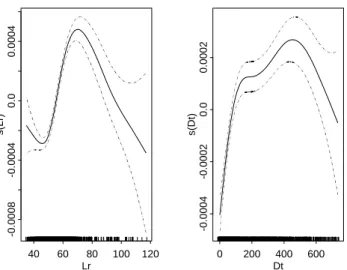
GAM results showed that the shape of the smoothed term for the length at release was roughly similar to the
average pattern of growth rate (Figure 6). GAM outputs showed a strong positive linear effect on the
transformed growth rate from 1 to 120-130 day at sea, an increasing effect until 500 days, then a decreasing trend for time at liberty larger than 550 d. The fact that the majority of time at liberty was smaller than 500 days suggests that the apparent growth rate is positively biased, i.e., overestimated. The optimal transformations
provided by a GAM produced a R2 of 0.26. The comparison between observed (i.e., apparent growth rates) and
fitted values is depicted in Figure 7. The predicted growth rate by size class when time at liberty was fixed at 1 is given in Table 2.
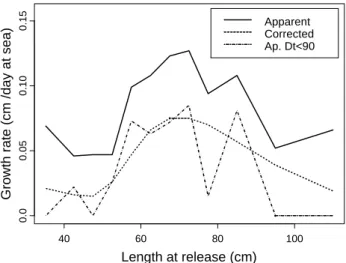
It must be stressed that if we consider only tagging data for which to time at liberty was shorter that 90 days, the apparent growth rate by size follows the same pattern and the same range than the GAM predicted values
(Figure 8); the large variability depicted by this variable was due to the small number of recaptures for some
size classes (unfortunately, for this reason it was not possible to use shorter time at liberty).
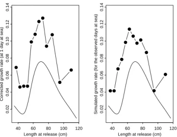
As mentioned in the Method section, to validate the GAM correction approach we simulated length at recapture by combining the predicted growth rate (assumed to be unbiased) with the median of times at liberty (i.e., the variable Dm in Table 2 observed for each size class in the data set. Then we compared the new simulated growth rates with the apparent growth rates observed previously.
Figure 9 shows that the same magnitude of overestimation exists between the apparent and the simulated growth
rates (in the left part and in the right part of the figure, respectively). So for species whose growth rate does not follow a linear decreasing trend over length, even if growth rate by size class is known perfectly, the resulting apparent growth rate will be biased. This similarity reinforces the usefulness of the correction procedure used to remove the bias caused by the time at liberty effect.
4. Discussion and conclusion
Studies supporting the two-stanza growth hypothesis were conducted in different oceans and locations were local recruitment was different, with different fishing gears and consequently with different selectivity patterns (Fonteneau, 1980, Bard 1984, Wild, 1986, Marsac and Lablache 1985, Gaertner and Pagavino, 1991, Lehodey and Leroy, 1999). Even if further studies are required to assess potential bias due to different factors (e.g., an effect of selectivity on the initial slow growth; a consequence of a sexual dimorphism in the growth, Wild 1986), the fact that different situations converge toward the same growth pattern suggests that the 2-stanza growth could be a characteristic of yellowfin tuna.
One of the assumptions raised by Fonteneau (1980) to explain the slow growth rate for juveniles is that grow could be stunted by limiting factors such as water temperature in the coastal areas or by trophic competition between individuals of many tuna species. As noted by Gaertner and Pagavino (1991), it was showed from biometric studies that yellowfin depicts important morphological transformations between 70 and 100 cm of fork length (Rossignol 1968, Baudin-Laurencin and Marchal 1968, Faure and Bablet 1982). Specifically, the increases in length of the second dorsal and the anal fins, as well as the posterior part of the body around 80 cm (Baudin-Laurencin and Marchal, op. cit) should be a condition to prepare the fish for future migrations offshore towards new areas with potentially different conditions of temperature, oxygen concentration, food, etc. Moreover, the development of the gas bladder associated with the increase in size (fish smaller than 50-60 cm, has no gas in the bladder) likely reduces drastically the energy requirement necessary to sustain the swimming (Lehodey and Leroy (1999). Such transformation corresponds to a change in the behavior of yellowfin (the fish moving deeper) and could indicate an extension of the habitat.
Constraining the growth to follow an inadequate model could have implications for stock assessments. In the lack of a satisfactory growth model which accurately accounts for the inflexion part of the curve, the use of growth rate by size class intervals appears as a reasonable approach. However as evidenced in this paper, the apparent growth rate does not represent the instantaneous growth rate at the length of release but an average pattern which depends on the time at liberty. We believe that the same problem occurs for hard part reading since apparent growth rates for large fish cannot reflect changes in growth rates which have occurred sooner at lower size classes. In the case of tagging data, we propose to remove the bias by using a fitted GAM model with time at liberty fixed at 1 day at sea.
References
Bard, F.X. 1984, Aspcct de la croissance de I'albacore Est-Atlantique (Thunnus albacares) à partir des marquages. Collect. Vol. Sci. Pap. ICCAT, 21: 108-114.
Bard, F.X., Chabanet, C., Caouder, N. 1991, Croissance du thon albacore (Thunnus albacares) en océan Atlantique estimée par marquages. Collect. Vol. Sci. Pap. ICCAT, 36: 182-204.
Baudin-Laurencin, F., Marchal, E. 1968, Contribution à l’étude biométrique de l’albacore Thunnus albacares du Golfe de Guinée. Doc. Sci. (Prov) C.R.O. Abidjan 24, 22p + unpag.
Bayliff, W.H. 1988, Growth of skipjack, Katsuwonus pelamis, and yellowfin, Thunnus albacares, tunas in the eastern Pacific Ocean, as estimated from tagging data. Interam. Trop. Tuna Comm. Bull. 19, 4, 311-385. Brouard, F., Grandperrin, R., Cillaurren, E. 1984, Croissance des jeunes thons jaunes (Thunnus albacares) et des
bonites (Katsuwonus pelamis) dans le Pacifique tropical occidental. ORSTOM de Port-Vila, Notes et Documents d'Oceanographie. 10, 1-23
Faure, E., Bablet, J.P. 1982, Contribution à l’étude des caractères biométriques du thon à nageoires jaunes du
Pacifique, Thunnus albacares (Bonnaterre, 1788). Cybium 3e ser., 6 (4), 31-55
Fonteneau, A. 1980, Croissance de l’albacore (Thunnus albacares) de l’Atlantique est. Collect. Vol. Sci. Pap. ICCAT, 9(1): 152-168.
Fonteneau, A., Gascuel, D. 2008, Growth rates and apparent growth curves, for yellowfin, skipjack and bigeye tagged and recovered in the Indian Ocean during the IOTTP. Sci. Doc. IOTC-2008-WPTDA-08.
Gaertner, D., Pagavino, M. 1991, Observations sur la croissance de l’albacore (Thunnus albacares) dans l’Atlantique ouest. Collect. Vol. Sci. Pap. ICCAT, 36: 479-505.
Gascuel, D., Fonteneau, A., Capisano, C. 1992, Modélisation d'une croissance en deux stances chez l'albacore (Thunnus albacares) de l'Atlantique est. Aquatic Living Resources, 5 (3): 155-172.
Le Guen, J.C., Sakagaua, G.T. 1973, Apparent growth of yellowfin tuna from the eastern Atlantic. Fish. Bull. 71, 175-187.
Lehodey, P., Leroy, B. 1999, Age and growth of yellowfin tuna (Thunnus albacores) from the western and central Pacific Ocean as indicated by daily growth increments and tagging data. SCTB12-WP YFT-2, 21 p.
Lessa, R., Duarte-Neto, P. 2004, Age and growth of yellowfin tuna (Thunnus albacares) in the western equatorial Atlantic, using dorsal fin spines. Fisheries Research, 69: 157-170.
Marsac, F., Lablache, G. 1985, Preliminary study of the growth of yellowfin (Thunnus albacares) estimated from purse seine data in the western Indian Ocean. FAO TWS/85/31.
Rossignol, M. 1968, Le thon à nageoires jaunes de l’Atlantique, Thunnus (Neothunnus) albacares (Bonnaterre) 1788. Mem. ORSTOM Paris, 25, 1-117.
Shuford, R.L., Dean, J.M., Stéquert, B., Morize, E. 2007, Age and growth of yellowfin tuna in the Atlantic Ocean. Collect. Vol. Sci. Pap. ICCAT, 60(1): 330-341
Venables, W.N., Ripley, B.D. 2002. Modern Applied Statistics with S, 4th ed. Springer-Verlag, New York, p. 495.
Wild, A. 1986, Growth of yellowfin tuna, Thunnus albacares, in the eastern Pacific Ocean based on otolith increments. Interam. Trop. Tuna Comm. Bull. 18, 6, 423-482.
Yang, R.T., Nose, Y., Hiyama, Y. 1969, A comparative study on the age and growth of yellowfin tunas from the Pacific and Atlantic Ocean. Bull. Far Seas Fish. Res. Lab., (2):1–21
Table 1. Example of simulation of the length at recapture for an hypothetical yellowfin tagged and released (Lr)
at 47 cm (FL) and let at sea for 180 days (D). g = apparent growth rate (averaged from both oceans); Ldl = size interval (or Lsup-Lr, for the 1rt interval); DL = time spent to grow from Linf to Lsup, at a specific size class growth rate; Dlive =D- Σ(DL) = time to live before the recapture; Lc=Length-at-recapture; g. sim= simulated growth rate.
_________________________________________________________________
Stepj Linf Lsup g Ldl DL Dlive Lc g. sim _________________________________________________________________ 1 35 40 0.058 0 0.00 180.00 2 40 45 0.042 0 0.00 180.00 3 45 50 0.057 3 52.52 127.48 4 50 55 0.065 5 77.28 50.20 5 55 60 0.081 5 61.89 -11.69 59.06 0.07 6 60 65 0.107 5 46.88 7 65 70 0.117 5 42.60 8 70 75 0.118 5 42.31 9 75 80 0.109 5 45.96 10 80 90 0.099 10 100.58 11 90 100 0.081 10 123.37 __________________________________________________________________
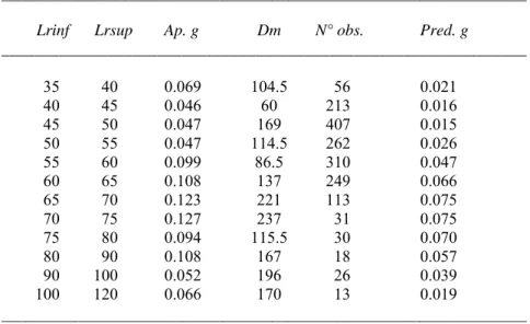
Table 2. Apparent and GAM predicted growth rates for yellowfin tuna in the Atlantic and in the Indian Ocean
from tagging data. Ap. g = apparent growth rate, Dm = median of the time at liberty for the corresponding size class (for length at release), N° obs= number of observations; Pred. g = GAM predicted growth rate for one day at sea.
________________________________________________________________
Lrinf Lrsup Ap. g Dm N° obs. Pred. g ________________________________________________________________ 35 40 0.069 104.5 56 0.021 40 45 0.046 60 213 0.016 45 50 0.047 169 407 0.015 50 55 0.047 114.5 262 0.026 55 60 0.099 86.5 310 0.047 60 65 0.108 137 249 0.066 65 70 0.123 221 113 0.075 70 75 0.127 237 31 0.075 75 80 0.094 115.5 30 0.070 80 90 0.108 167 18 0.057 90 100 0.052 196 26 0.039 100 120 0.066 170 13 0.019 ________________________________________________________________
40 60 80 100 0. 0 0 .2 5 G . ra te (cm) Length at release (cm) 40 60 80 100 0. 0 0 .2 5 G . ra te (cm) Length at release (cm) 40 60 80 100 0. 0 0 .2 5 G . ra te (cm) Length at release (cm) 40 50 60 70 0. 0 0 .2 5 G . ra te (cm) Length at release (cm) 40 60 80 100 0. 0 0 .2 5 G . ra te (cm) Length at release (cm) 40 60 80 100 120 140 0. 0 0 .2 5 G . ra te (cm) Length at release (cm) 40 60 80 100 120 0. 0 0 .2 5 G . ra te (cm) Length at release (cm) 40 60 80 100 120 0. 0 0 .2 5 G . ra te (cm) Length at release (cm)
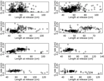
Figure 1. Apparent growth rate (cm d-1) over length at recapture (cm) by quarters of time at liberty (from Qt <=1
in the upper left part to Qt >=8 in the lower right part) for yellowfin tuna in the Atlantic and in the Indian Ocean.
4.380 4.381 4.382 4.383 4.384 4.385 0 100 200 300 400 500 600
Growth rate (cm / day at sea)
Densi
ty
40 60 80 100 120 0.0 0 .05 0 .10 0 .15 0 .20 0 .25 0 .30 G. rate (cm) Length at release (cm) 40 60 80 100 120 0.0 0 .05 0 .10 0 .15 0 .20 0 .25 0 .30 G. ra te (c m) Length at release (cm)
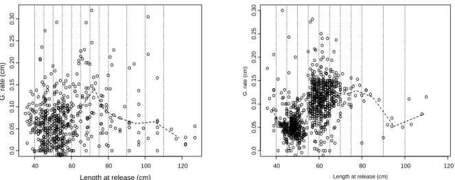
Figure 3. Apparent growth rate (cm d-1) over length at release (FL in cm) for yellowfin tuna in the Atlantic (in
the left) and in the Indian Ocean (in the right). The broken line represents the medians of growth rate by size class. 40 60 80 100 0.0 0 .05 0 .10 0 .15 Length at release (cm)
Growth rate (cm /day at sea)
Mean Atlantic Indian O.
Figure 4. Apparent average growth rate (cm d-1) for yellowfin tuna inferred from tagging data obtained in the
Length at release 40 50 60 70 80 0.0 0 .04 0 .10 Gr owth r a te ( c m /day at sea) Days at sea = 10 Length at release 40 50 60 70 80 0.0 0 .04 0 .10 Gr owth r a te ( c m /day at sea) Days at sea = 180 Length at release 40 50 60 70 80 0.0 0 .04 0 .10 Gr owth r a te ( c m /day at sea) Days at sea = 360 Length at release 40 50 60 70 80 0.0 0 .04 0 .10 Gr owth r a te ( c m /day at sea) Days at sea = 540
Figure 5. Simulated changes in the apparent growth rate (cm day-1) of yellowfin for different days at sea (10,
180, 360 and 540 d). The lines with points represent the values of the apparent average growth rate by size class of 5 cm used as initial growth rates by size for the simulation.
Lr s( Lr ) 40 60 80 100 120 -0.0008 -0.0004 0.0 0 .0004 Dt s( Dt) 0 200 400 600 -0.0004 -0.0002 0.0 0 .0002
Figure 6. Generalized additive model (GAM) derived relationships between length at release (Lr) and time at
Length at release (cm) 40 60 80 100 120 0.0 0 .02 0 .06 0 .10 0 .14 Growth rate Observed Fitted
Figure 7. Observed and GAM fitted values for the apparent growth rate (cm d-1) of yellowfin tuna inferred
from tagging data in the Atlantic and in the Indian Oceans.
40 60 80 100 0.0 0 .05 0 .10 0 .15 Length at release (cm)
Growth rate (cm /day at sea)
Apparent Corrected Ap. Dt<90
Figure 8. Change in growth rate for yellowfin tuna from combined tagging data (Atlantic and Indian Ocean).
Apparent = observed growth rate by length class; Ap. D<90 = observed growth rate for time at liberty shorter than 90 day at sea; Corrected = predicted growth rate from a GAM assuming 1 day at liberty.
Length at release (cm) 40 60 80 100 120 0.02 0.04 0.06 0.08 0.10 0.12 0.14 Cor re cted gr owth r a te ( a t 1 day at sea) Length at release (cm) 40 60 80 100 120 0.02 0.04 0.06 0.08 0.10 0.12 0.14 Si mul ated gr owth r a te ( for the obser
ved days at sea)
Figure 9. Comparison between the corrected growth rate (predicted values from a GAM in which time at
liberty was fixed at one day at sea) represented by the continuous line, the observed apparent growth rate (in the left figure) and the simulated growth rate (in the right figure) calculated by combining the GAM corrected growth rate and the observed median time at liberty by size class.