A Long-Term Electricity Dispatch Model with the TIMES
Framework
Ramachandran Kannan&Hal Turton
Received: 17 October 2011 / Accepted: 17 September 2012 # Springer Science+Business Media Dordrecht 2012
Abstract A new Swiss TIMES (The Integrated MARKAL– EFOM System) electricity model with an hourly representation of inter-temporal detail and a century-long model horizon has been developed to explore the TIMES framework’s suitability as a long-term electricity dispatch model. To understand the incremental insights from this hourly model, it is compared to an aggregated model with only two diurnal timeslices like in most MARKAL/TIMES models. Two scenarios have been analysed with both models to answer the following questions: Are there differences in model solutions? What are the benefits of having a high number of timeslices? Are there any compu-tational limitations? The primary objective of this paper is to understand the differences between the solutions of the two models, rather than Swiss policy implication or potential uncer-tainties in input parameters and assumptions. The analysis reveals that the hourly model offers powerful insights into the electricity generation schedule. Nevertheless, the TIMES framework cannot substitute for a dispatch model because some features cannot be represented; however, the long model time horizon and integrated system approaches of TIMES provide features not available in conventional dispatch models. The methodology of the model development and insights from the model comparison are described.
Keywords Energy systems model . Electricity . TIMES . Dispatch model . Switzerland . STEM-E
1 Introduction
Numerous energy models covering a wide range of analyt-ical approaches have been developed [14,25]. Energy mod-elling frameworks are often developed for specific objectives, with a predefined methodological scope and limited application [28]. For example, in Switzerland, a range of top-down energy-economy models [3, 4, 7, 11,
15–18,43], bottom-up energy systems models [9,22] and sector-specific energy/electricity models [2,24,30,39,46,
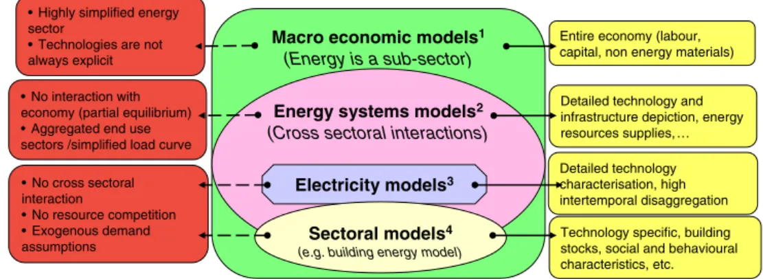
49, 51] have been developed for analysing energy and climate change mitigation policies. Some of the models are rich in the level of technological detail, while others have a greater focus on the representation of energy-economy link-ages. The objectives and scope of these models (Fig.1) are diverse, with different strengths and weakness, providing complementary insights on a range of aspects of the energy system.
One of the key attributes that distinguishes different bottom-up energy models is temporal depiction. The tem-poral representation has three dimensions: (1) the model time horizon; (2) flexibility in period definition (e.g. prede-fined periods, choice of fixed (equal) period length, options for unequal period length) and (3) flexibility in intra-annual time resolution.
The model time horizon is critical when the research is concerned with long-term energy challenges such as re-source depletion, technology spill over effects, climate change mitigation policy, infrastructure evolution and so on. Clearly, uncertainties affecting the energy system in-crease over longer model time horizons, as we deal with uncertain future parameters, like economic growth, technol-ogy development and energy demands. In some modelling frameworks [50], these long-term uncertainties can be rep-resented while maintaining a greater focus on near- to mid-term developments, through the definition of unequal time
R. Kannan (*)
:
H. TurtonEnergy Economics Group, Laboratory for Energy Systems Analysis, Paul Scherrer Institut,
5232 Villigen, Switzerland e-mail: [email protected] R. Kannan e-mail: [email protected] H. Turton e-mail: [email protected]
Environ Model Assess (2013) 18:325–343 DOI 10.1007/s10666-012-9346-y
periods in the model, describing the near term in a higher level of temporal detail. Finally, the intra-annual time resolution (i.e. the level of temporal detail within a year) is important when the energy system needs timely supply of energy com-modities, which cannot be easily or cost-effectively stored. For example, electricity is a highly time-dependent energy commodity because both energy and capacity demands must be met at every instant. Therefore, electricity system models require detailed intra-annual time resolution to represent the dynamics of demand and supply.
Energy system models conventionally adopt a long time horizon but have a very limited intra-annual time resolution. In contrast, electricity dispatch models [26] often have high levels of intra-annual time resolution although their time horizon is limited. In an earlier publication [38], we dis-cussed the importance of these two temporal dimensions. Ideally, models of energy system development should com-bine a sufficiently long time horizon and an appropriate level of intra-temporal resolution for the given analysis. In practical terms, the trade-offs between these two temporal dimensions are driven by a range of factors including: computational resources, solver algorithm capabilities, data availability and methodological limitations within the mod-elling framework, which may have a limited set of possible time-dependent variables and be able to deal only with limited types of energy commodity [28,31,38]. The review from Boqiang and Chuanwen [10] acknowledges the com-plexities in modelling the long-term and short-term sched-uling of electricity supply. Importantly, these modelling trade-offs could also affect model solutions, and thus it is important to find the right balance given the practical con-straints and the specific analytical policy application. Some approaches combine two or more modelling frameworks to integrate the two temporal aspects [13,31].
Advances in computational power and solver algorithms have facilitated the emergence of modelling frameworks
combining a long time horizon and detailed intra-annual time resolution for representing electricity load curves. As an earlier attempt, a‘flexible timeslicing’ feature was intro-duced in the MARKAL (market allocation) framework [41,
45], enabling more detailed representation of variations in energy demand and supply, including operating character-istics of specific technologies. This flexible timeslicing was first implemented in the UK MARKAL model [38] and the analyses concluded that the higher number of timeslices alone was not sufficient to represent grid balancing mecha-nisms because the electricity storage formulation was still only capable of dealing with one diurnal timeslice. This particular limitation is addressed in The Integrated MAR-KAL–EFOM System (TIMES) framework [42]. TIMES builds on the best features of MARKAL [41] and the energy flow optimization model (EFOM) [50]. The TIMES frame-work has the capacity to represent any number of intra-annual timeslices and unequal time periods. It is also enhanced to depict energy storage for any type of energy commodity (e.g. electricity or gas storage for peak demands). This allows, for example, the representation of pumped hydroelectric storage used to store electricity during one timeslice and release it during another. Notably, this storage feature is often not in-cluded in electricity dispatch models.
The TIMES framework has been extensively applied for energy system modelling, and has proven useful for a range of national, regional and global analyses [23]. In this paper, we take the TIMES framework a step further and explore its suitability to represent electricity dispatch and substitute (to some degree) for a dispatch model. We have developed a Swiss TIMES electricity systems model (STEM-E) with an hourly timeslice resolution and a century-long time horizon with unequal time periods [33, 34, 36, 37]. The primary objective of developing STEM-E is to understand the long-term evolution of the Swiss electricity system. At the same time, it is intended to provide insights into electricity
Macro economic models1
(Energy is a sub-sector)
Energy systems models2
(Cross sectoral interactions)
Electricity models3
Sectoral models4
(e.g. building energy model)
Detailed technology and infrastructure depiction, energy resources supplies, … Detailed technology characterisation, high intertemporal disaggregation Technology specific, building stocks, social and behavioural characteristics, etc. Entire economy (labour, capital, non energy materials) • Highly simplified energy
sector
• Technologies are not always explicit • No interaction with economy (partial equilibrium) • Aggregated end use sectors /simplified load curve • No cross sectoral interaction
• No resource competition • Exogenous demand assumptions
Fig. 1 Overview of the existing Swiss modelling tools and framework. 1 CGE [7,16], CITE [11], Geneswis [15], GEMINI-E3 [4,40], GEM-E3 [3], MultiSWISSEnergy [7], MERGE [43], Global Trade Analysis Project (GTAP) [18], SwissOLG [17], SwissGem [16]. 2 MARKAL
[22,39], ETEM [21,40], TIMES [9]. 3 MARKAL electricity model [51], Electricity trade model [2], System dynamics model [46] Prognos [49], DIME [24]. 4 Building energy model [30], SMEDE [39]
generation scheduling by accounting for availability and operational constrains of different generation technologies. In this paper, we seek to determine the incremental insights provided by this hourly model by comparing it to a standard TIMES model with eight annual timeslices (i.e. four sea-sonal and two diurnal). We analyse two scenarios in each model and compare the results to answer the following questions: Are there differences in model solutions? What are the benefits of having a high number timeslices? Are there any computational limitations and complexities? An important caveat in this analysis is that the scenarios pre-sented are examples intended for illustrating and explaining methodological difference between the two modelling approaches, rather than representing specific Swiss electric-ity polices which are extensively analysed in STEM-E and presented in our other publications [33,56].
The paper is organised as follows: Section2provides an overview of the development, features and key input assumptions of STEM-E; Section3 describes the aggrega-tion of the hourly timeslices in STEM-E into two diurnal timeslices to create a‘standard’ TIMES model for compar-ison; Section4 describes the scenario analysis and results; Section5compares and discusses the findings in the context of the questions outlined above and suggests an outlook for future analyses; while Section6draws key conclusions.
2 Swiss TIMES Electricity Model
2.1 STEM-E Model Definition
TIMES is a bottom-up, dynamic, cost-optimisation model-ling framework [42]. TIMES, like its predecessor MAR-KAL [41], has the capability to portray the entire energy system. TIMES determines the system-wide cost-optimal evolution of the energy system, and thus provides an ideal framework for developing a vertically integrated model of the entire energy system. However, TIMES is also suitable for modelling in detail individual subsectors of the energy system, such as the electricity system.
STEM-E is a single-region model, covering the entire Swiss electricity system from resource supply to end use. A reference energy system connects energy resources, con-version technologies and end-use demand through different energy commodities. Primary energy resources in the model comprise renewable and imported fuels, which are used as inputs to the electricity generation technologies. Electricity outputs from the electricity and combined heat1and power (CHP) generation technologies are distributed to end-use
sectors. CO2 emissions from fossil fuels are tracked at the
resource consumption level. To understand the role of inter-national electricity trade, STEM-E has four explicit electricity interconnectors representing trade with Austria, Germany, France and Italy (further described in Section2.2.3).
The model is fully calibrated to historical data [5, 6] between 2000 and 2009 for electricity supply, demand, generation mix and capital stock. The model has a range of user-defined constraints to reflect historical operational characteristics, technical and resources availability, market share and so on. It was not possible to obtain historical data at an hourly level. Therefore, the model is calibrated to annual and seasonal electricity generation data, but avail-ability factors are implemented at the weekly, daily and hourly levels to imitate historical electricity system charac-teristics. All cost data in the model are reported in 2010 Swiss Francs (CHF2010).2The model uses a discount rate of
3 % reflecting the real long-term yield from Swiss confed-eration bonds plus an additional risk premium for energy sector investments [54].
2.1.1 Temporal Depiction
The model has a time horizon of 110 years (2000–2110) in 14 unequal time periods. The time periods are specified to a length of 2 years in the short term to enable detailed cali-bration to the historical data. In the medium and long term, the period is specified to be between 5 and 20 years in length (Table1).
The intra-annual timeslices are depicted at seasonal, daily and hourly levels. The number of timeslices was decided based on analysis of Swiss electricity demand curves. Figure2 presents Swiss hourly electricity demand [20] for the year 2008 aggregated at four seasonal and three daily levels. There is a considerable difference between the lowest and the highest demands across seasons (peaking around 2 GW higher on winter weekdays than in summer), between days of the week (weekdays vs. weekends), and even within each day. For example, on summer weekdays there is a very steep increase in demand of around 1.5 GW from around 6 am to the peak at close to 12 pm. Across the weekdays there is some variation in load profile (not shown), but the shape of the load curves is more or less similar. On Satur-days and SunSatur-days, the demand pattern is slightly different from the weekdays. For instance, on winter Saturdays the peak load occurs at 1 am and at a lower level than on weekdays. On summer Saturdays, the demand pattern is similar to the summer weekdays except there is no large daytime peak. For STEM-E, 4 seasonal, 3 daily and 24 hourly timeslices have been chosen. Thus the model has 288 annual timeslices as illustrated in Fig.3. Table2shows 1
There is no heat demand in the model. In order to cope with operation of CHP, heat output from CHPs is currently modelled to be exported
the seasonal descriptions and the annual fraction of time-slices (i.e. the QHR(Z)(F) parameter in [41,42]).
2.2 Reference Energy System
2.2.1 Electricity End-Use Sectors
Electricity demands from five end-use sectors are given exogenously. Future electricity demands during 2011–2035 are assumed based on the growth projections from the Scenario I of the Energy Perspectives [7]. For all the end-use sectors, electricity demand is assumed to follow the Swiss load curve because data on sectoral load curves were not found. Analysis of the historical load curves [20] reveals that the‘load profile’ has not changed significantly in the recent past (2000–2009) even though the total ‘electricity demand’ has changed. Thus, the year 2008 load curve is applied for the entire model horizon, although continuing electrification and demands from emerging technologies (e.g. battery or plug-in hybrid vehicles) could affect this assumption.
2.2.2 Electricity Generation Technologies
Electricity supplied to end-use sectors can be produced with a range of existing and new electricity (and heat3) genera-tion technologies. Operagenera-tional characterisagenera-tion of electricity generation technologies in TIMES is same as in the MAR-KAL framework (see [35,38]). All existing electricity gen-eration technologies in the Swiss electricity system have
been modelled at an individual plant level or as a group aggregated by fuel and technology. Capacity factors for all the existing technologies have been calculated for the past 10 years for individual or aggregated groups of technolo-gies. The statistical average capacity factor is applied as the availability factor (of the existing technology) for the future years. For the existing technologies, operation and mainte-nance (O&M) costs are accounted using the same values as in the future technology data (see [34]).
All the existing nuclear reactors are modelled as base-load plants and scheduled to retire 50 years after installation. The federal levies for decommissioning (2 CHF/MWh) and waste disposal (8 CHF/MWh) [8] are applied as a tax to the electricity generated from nuclear plants. Run-of-river hydro plants are characterised as seasonal base-load plants with seasonal availability factors. The model has the flexibility to schedule the run-of-river hydro at varying load at seasonal level while fulfilling the seasonal and annual availability of run-of-river hydro resources. The dam and pumped hydro plants are characterised as flexible (dispatchable) technolo-gies. For the dam hydro plants, availability factors are implemented at the daily level to reflect the historical oper-ational characteristics. Most of the existing thermal power plants (oil-, gas- and biomass-fired CHP plants; and waste incineration plants) and geothermal plants are characterised as a seasonal base-load plants.
Wind turbines are characterised as seasonal base-load plants with different seasonal availability factors (because hourly wind resource data are unavailable). Based on monthly average wind speeds from selected locations [57] the seasonal share of wind energy (i.e. square of the wind speed) is normalised to a 14 % annual capacity factor [53]. The seasonal availability in winter (18 %) is generally higher than in summer (10 %). Hourly wind data from one potential wind site [44] shows some variations in seasonal hourly availability (in the range of 16–20 % in winter and 5– 10 % in summer). It is proposed to implement this hourly profile in future versions of the model.
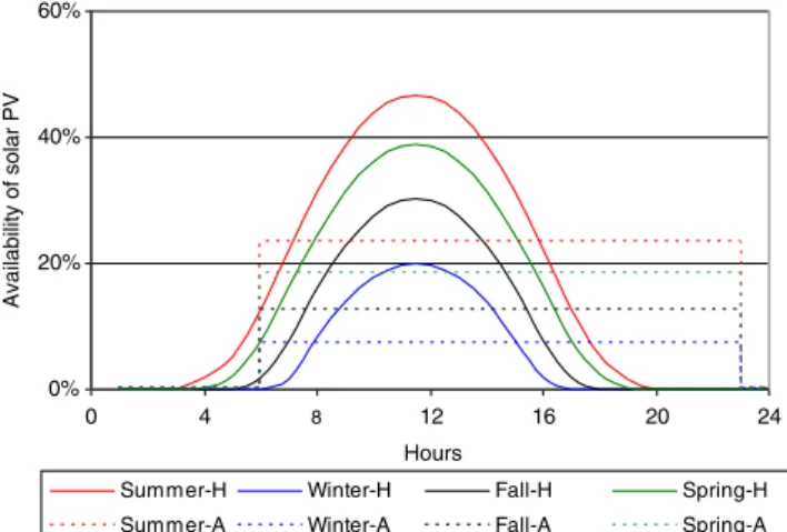
For solar PV, hourly solar irradiation from selected loca-tions [32] is normalised to the annual capacity factor of solar PV. This availability factor is implemented at the hourly timeslice level (Fig.7).
For pumped hydro, a dedicated storage process is defined as an inter-timeslice storage technology. With this formula-tion, electricity can be stored and discharged within any timeslice, overcoming one of the limitations in the MAR-KAL framework (also see [38]). The output from the storage technology feeds the pumped hydro power plant.
A range of new electricity generation technologies are available in three vintage years: 2010, 2030 and 2050. Technical and cost data of the new technologies are adopted from [48] and summarised in Fig. 4. The existing hydro plants are assumed to be refurbished at 35 % cost of new-3
See footnote 1.
Table 1 Unequal modelling time horizon in STEM-E Period number Period length (years) Actual time periods Milestone yeara 1 1 2000–2000 2000 2 2 2001–2002 2001 3 2 2003–2004 2003 4 2 2005–2006 2005 5 2 2007–2008 2007 6 4 2009–2012 2010 7 5 2013–2017 2015 8 5 2018–2022 2020 9 6 2023–2028 2025 10 12 2029–2040 2034 11 15 2041–2055 2048 12 15 2056–2070 2063 13 20 2071–2090 2080 14 20 2091–2110 2100 a
build hydro plants. Construction and decommissioning times are included for all the large-scale power plants to account for lead times and interest costs incurred during construction. In TIMES, the capital cost is assumed to be paid uniformly over the construction time.
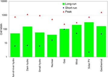
Based on the 2010 technology and fuel costs, long-run, short-run and peak time costs of electricity are shown in Fig.5. The long-run cost is typically the levelised cost. The short-run cost is based on variable O&M cost and fuel costs only. The peak electricity cost is calculated to reflect the cost of meeting a 1-h peak time demand. It is calculated by assuming that the plant is used for only 1 kWh over its lifetime. It can be seen that capital-intensive technologies have a low long-run cost and a high peak marginal cost. Although TIMES is a cost-optimisation model, technology choice is determined not only on a single measure of cost, but also according to flexibility that determines the
suitability of a technology for supplying dynamic demands. The different cost estimates presented in Fig. 5 help to illustrate how different technologies may be more cost com-petitive under different patterns of demand, compared to a simple ranking based on levelised cost.
2.2.3 Energy Resources
Energy resource potential and cost assumptions are taken from a range of sources (e.g. [22,29,48,53]) and given in the model documentation [34]. For renewables, resources potentials are implemented at the level of the conversion technologies.
The Swiss electricity network is connected to the EU network via four bordering countries (Austria, France, Ger-many and Italy) [19, 20]. Switzerland is self-sufficient in meeting its annual electricity demand, but reliant on
Weekdays 3 4 5 6 7 8 0 6 12 18 24 GW Winter Spring Summer Fall Saturdays 3 4 5 6 7 8 0 6 12 18 24 GW Winter Spring Summer Fall Sundays 3 4 5 6 7 8 0 6 12 18 24 GW Winter Spring Summer Fall
Fig. 2 Swiss seasonal and daily electricity load curves (2008) Daily (12) SPR-W K Winter Sunday SPR-S A SPR-S U SUM -WK SUM -S A SUM -SU FA L-W K FA L-SA FA L-SU WIN -WK WIN-SA WIN-SU Hourly (288) SPR -W K -D01
Winter - Sunday - midnight
SPR -W K -D02 SPR -W K -D03 SPR-W K -D04 SPR-W K -D05 SPR-W K -D23 SPR -W K -D24 WI N-S A -D01 WI N -SA -D02 WI N-S A -D03 WI N-SA -D04 WI N -SA -D05 W IN-SA -D23 WI N-SA -D24 Milestone year 2100 2041-55 2013-17 2001-02 2000 Model horizon (2000 – 2110) 2091 - 2110 Seasonal (4) Winter
Spring Summer Fall
WK- Weekdays, SA- Saturdays SU- Sundays D01 to D24 – daily hours Daily (12) SPR-W K Winter Sunday SPR-S A SPR-S U SUM -WK SUM -S A SUM -SU FA L-W K FA L-SA FA L-SU WIN -WK WIN-SA WIN-SU Hourly (288) SPR -W K -D01
Winter - Sunday - midnight
SPR -W K -D02 SPR -W K -D03 SPR-W K -D04 SPR-W K -D05 SPR-W K -D23 SPR -W K -D24 WI N-S A -D01 WI N -SA -D02 WI N-S A -D03 WI N-SA -D04 WI N -SA -D05 W IN-SA -D23 WI N-SA -D24 Milestone year 2100 2041-55 2013-17 2001-02 2000 Model horizon (2000 – 2110) 2091 - 2110 Seasonal (4) Winter
Spring Summer Fall
WK- Weekdays, SA- Saturdays SU- Sundays
D01 to D24 – daily hours
Fig. 3 Temporal depiction tree in STEM-E. Modified from Remme and Blesl [52]
imported electricity for certain seasons (e.g. winter). It trades large amounts of electricity, particularly importing cheap off-peak electricity and exporting during off-peak hours using its large dam and pumped hydro facilities. For example, Switzerland imported 66.3 TWh of electricity in 2010 at an average price of 56 CHF/MWh and exported 66.6 TWh at 76.5 CHF/MWh. This trade generated a net revenue of CHF 1.3 billion [5]. The electricity trade volume varies by country and season. About 80 % of the electricity export is to Italy and imports are from Germany (46 %), France (32 %) and Austria (22 %) [20]. Electricity export to Germany and France occurs mainly dur-ing peak hours. In STEM-E, four country-specific electric import and export resources are defined to represent these four markets and linked to the Swiss network via dedicated interconnectors. The interconnectors are modelled as flexible4 technologies so that electricity can be traded at any time. Much of the current international electricity trading is to exploit price differentials at a given time in the countries bordering Switzerland. However, STEM-E is not intended to analyse electricity trading from this arbitrage perspective. Instead the model is intended to account for the effect of trade on the operational sched-ule of power plants, and the possibilities to import
cheap off-peak electricity, store this electricity via pumped storage and export it during periods with higher prices.
There are large uncertainties and volatility in the electric-ity trade price. We use the electricelectric-ity demand curves from the four countries to estimate country-specific prices for each timeslice and implement a cost coefficient for all 288 timeslices as a function of an annual electricity import price.5 These estimates are derived by multiplying the an-nual electricity price [1] by a timeslice coefficient. This coefficient is a linear function of the capacity demanded, calculated from the fraction of annual demand in a given timeslice divided by the proportion of the year represented by the timeslice. Thus, if the hourly demand fraction is higher than the hourly fraction, the electricity cost at that timeslice is high and vice versa. The rationale for this approach is that electricity price is expected to be higher when demand is higher. For each of the four neighbouring countries, the electricity export price in each timeslice is pegged to the import price.
Interconnector capacity is limited to not more than 150 % of today’s level by 2050 and 200 % by 2100. In addition, country-specific market shares are also implemented based
4This assumption provides flexible exchange of electricity in the future years, but the future availability of interconnectors is quite uncertain and heavily dependent on electricity system development in the four markets.
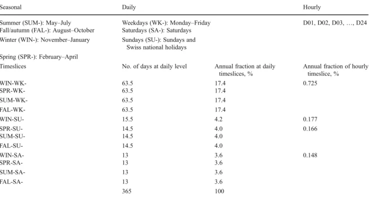
5We analysed hourly electricity spot market prices for 2008 [19] and generated dependent electricity import prices for all the 288 time-slices. However, this approach did not imitate the historical trade pattern. Thus, the current approach is implemented to model the trading mecha-nism, but this represents an area of further model development. Table 2 Definition of inter annual timeslices
Seasonal Daily Hourly
Summer (SUM-): May–July Weekdays (WK-): Monday–Friday D01, D02, D03,…, D24
Fall/autumn (FAL-): August–October Saturdays (SA-): Saturdays Winter (WIN-): November–January Sundays (SU-): Sundays and
Swiss national holidays Spring (SPR-): February–April
Timeslices No. of days at daily level Annual fraction at daily
timeslices, %
Annual fraction of hourly timeslice, % WIN-WK- 63.5 17.4 0.725 SPR-WK- 63.5 17.4 SUM-WK- 63.5 17.4 FAL-WK- 63.5 17.4 WIN-SU- 15.5 4.2 0.177 SPR-SU- 14.5 4.0 0.166 SUM-SU- 14.5 4.0 FAL-SU- 14.5 4.0 WIN-SA- 13 3.6 0.148 SPR-SA- 13 3.6 SUM-SA- 13 3.6 FAL-SA- 13 3.6 365 100
on the historical trade volumes [19]. The combined electric-ity import and export volume is also limited to 250 PJ, which is 20 % more than the historical trade volume. With the limits on interconnector capacity expansion, and region-al electricity market share, arbitrage-driven trade effects are curtailed.
3 Aggregated STEM-E Model
To understand the incremental insights from the hourly STEM-E model, a second version of the model is created in which the 288 timeslices are aggregated to a level similar to most TIMES/MARKAL models. The 24 hourly time-slices are aggregated to two timetime-slices via day (D01) and night (D02), while the representation of different days of the week is fully removed. The four seasons are retained. Thus the aggregated model has eight annual timeslices (Table3). All other inputs, e.g. technology characterisation, demands and cost data remain the same in both models. Nevertheless,
the following parameters have to be changed to reflect the intra-annual aggregations:
1. Yearly fraction (QHR(Z)(F)) and demand fractions (FHR(Z)(F)) are aggregated as in Table 3. Note, day (D01) is assumed to be 17 h (6 am–11 pm), and night (D02) 7 h (11 pm–6 am), in all seasons.
2. Figure6shows the load curve from the aggregated and hourly models for winter and summer seasons. The aggregation of hourly timeslices and the removal of the differentiation of weekdays and weekends reduce substantially the variation between the highest and low-est demand seen in the hourly model. This weekly aggregation thus underestimates the operational con-straints facing large base-load plants.
3. For solar PV, seasonal solar irradiation is allocated to the daytime (D01). Figure7shows the availability fac-tors of solar PV implemented in both models. It can be seen that the hourly model has a higher peak availability factor, though for a shorter duration. Although the sea-sonal electricity output from a given installed capacity of solar PV is the same in both models, the aggregated model offers a low capacity contribution because the
1 10 100 1000 10000 R u n-of -r iv er hy dr o Da m h y d ro S m al l hy dr o Nu c le a r Ga s Wi nd So la r PV Ge o th e rm a l CHF /M W h Long-run Short-run Peak
Fig. 5 Comparison of electricity generation costs based on 2010 data
Table 3 Fraction of year and demands in aggregated model
Timeslice (Z)(F) FHR(Z)(F), % QHR(Z)(F), % FAL-D01 18.5 17.7 FAL-D02 6.9 7.3 SPR-D01 17.6 17.7 SPR-D02 6.9 7.3 SUM-D01 15.1 17.7 SUM-D02 5.6 7.3 WIN-D01 20.8 17.7 WIN-D02 8.4 7.3
D01 daytime (6 am–11 pm), D02 nighttime (11 pm–6 am)
20% 40% 60% 80% 100% Efficiency Run-of-river hydro Dam hydro Small hydro Nuclear Gas Wind Solar PV Geothermal - 3,000 6,000 9,000 12,000 Capital cost (CHF/kW) Run-of-river hydro Dam hydro Small hydro Nuclear Gas Wind Solar PV Geothermal
output is spread uniformly over the daytime (17 versus 10 h in winter in the hourly model).
4. For electricity trade, new cost coefficients are imple-mented for eight timeslices using the same methodology described in Section 2.2.3. Due to this aggregation, there is much less variation in trade price reducing incentives for trade.
4 Results
A range of Swiss electricity policy scenario analyses have been undertaken with STEM-E [33, 56]. For this paper, however, the objective is to illustrate the differences be-tween the solutions of the two models, rather than Swiss
policy implication or potential uncertainties in input param-eters and assumptions.
4.1 Scenario Description
4.1.1 Base Scenario
The base scenario (Base) represents a least-cost Swiss elec-tricity system based on conventional and historical trends. As mentioned above, this scenario is intended to illustrate the methodology, rather than representing specific Swiss electricity polices.6To avoid excessive imports or exports and to reflect self-sufficiency in electricity supply, a con-straint is introduced requiring that net electricity trade is roughly in balance over the year. The timing of electricity trade is left unconstrained, but annual exports and imports are required to be roughly in balance.
4.1.2 Hyp Scenario
We also considered a hypothetical scenario (Hyp), con-structed to test potential strengths (and shortcomings) of the hourly model over the aggregated model. In this scenario new investment in dam hydro and electricity trade is pro-hibited, although existing capacities remain available to avoid the need for a recalibration. While large-scale flexible 0% 20% 40% 60% 0 4 8 12 16 20 24 Hours Availability of solar PV
Summer-H Winter-H Fall-H Spring-H Summer-A Winter-A Fall-A Spring-A
Fig. 7 Availability factor of solar PV in hourly (H) and aggregated (A) models
6For instance, in May 2011, the Swiss Federal council decided to completely restrict investment in new nuclear power plants. The Base scenario does not include this restriction, which has been analysed in our other publications [33,56]. Thus, we re-emphasise that the Base scenario is adopted as an illustrative case.
Winter 5.0 5.5 6.0 6.5 7.0 7.5 0 6 12 18 24 GW Weekdays Saturdays Sundays Aggregated Summer 3.5 4.0 4.5 5.0 5.5 6.0 0 6 12 18 24 GW Weekdays Saturdays Sundays Aggregated
Fig. 6 Electricity load curve in hourly model versus aggregated model
dam hydro and electricity trade play a crucial role in Swit-zerland in balancing demand fluctuations, these options are not available to the same extent in many countries. Thus, the Hyp scenario seeks to address more broadly the research question and the wider applicability of a TIMES model for dispatch modelling, by removing some of the features spe-cific to Switzerland (and which are very important for load balancing).7Clearly, Hyp is also not intended to represent a realistic technology scenario for Switzerland.
The Base and Hyp scenarios are analysed in both the models. The scenario from the aggregated model is denoted with suffix A (i.e. Base-A and Hyp-A). Since the primary objective of this paper is to understand the incremental benefit of the hourly model, the results are discussed to reveal the differences.
4.2 Generation Mix
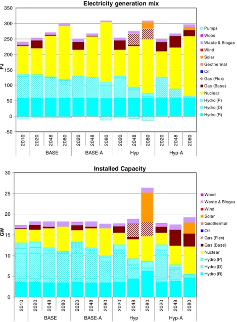
Figure88shows the electricity generation mix and installed capacity from both models. In the Base scenario, the short-term (through to 2020) supply gap is met with new invest-ments in gas-based generation capacity. In the medium and long run, the models choose nuclear capacity as the cost-effective supply option. By 2050, nuclear generation con-tributes to 50 % of the total generation while hydro (48 %) and renewables contribute the rest. The hourly and aggre-gated models choose a similar technology mix in the short and medium term because of large capital stocks (particu-larly, the long-life (80 year) hydro plants). In the long run, however, the aggregated model chooses a higher share of nuclear generation and a lower share of hydro. In 2080, the hourly model (Base scenario) chooses 58 % nuclear and 19 % dam hydro whereas the shares are 65 % and 14 %, respectively, in the aggregated model (Base-A scenario). Since there is less demand variation in the aggregated model (Fig. 6), the model installs a larger quantity of base-load (nuclear) capacity and smaller capacity of dispatchable tech-nologies like dam hydro. In particular, the absence of de-mand variations between weekdays and weekends enables a larger deployment of base-load generation. On the other hand, electricity trade volume in the aggregated model (Base-A scenario) is less than that in the hourly model (Base scenarios) (compare Figs. 9 and 10). In 2080, the
combination of the large base-load capacity and low trade volume induce some investments in pumped hydro in the Base-A scenario for load management.
In the Hyp scenarios, the models choose a similar gener-ation mix to some extent, although the choice of technology type differs. The hourly model invests in flexible (dispatchable) gas combined cycle (Gas (F) in Fig. 8) and pumped hydro power plants to cope with the dynamic load curve; whereas the aggregated model (Hyp-A scenario) chooses more base-load gas combined cycle plants (Gas (B) in Fig. 8). The base-load gas plant is chosen in the aggregated model because there is much less variation in demand across the day (Fig. 6); while this technology is assumed to have the flexibility to operate at different ‘sea-sonal’ load factors, which enables the model to cope with the seasonal demand variations (whereas nuclear plant is not assumed to have such seasonal operational flexibility). Like in the Base-A scenario, the large capacity of base-load generation (nuclear and gas) in the Hyp-A scenario easily copes with the narrow variation between day and night demands.
In the long term (2080), solar PV technology becomes cost-effective because the cost of this technology is assumed to decline, while the gas price is assumed to increase (and capacity of nuclear plant is capped (7 GW)). In 2080, the installed capacity of solar PV in the hourly model (Hyp scenario) is 7.3 GW compared to 2.8 GW in the aggregated model (Hyp-A scenario). The underlying drivers are further explained in the generation schedule in Section4.3.2.
4.3 Electricity Dispatch Schedule
The advantage of the hourly model is its capability to provide insights on the scheduling of generation capacity. This section explains the underlying drivers of generation scheduling from both models.
4.3.1 Base and Base-A Scenarios
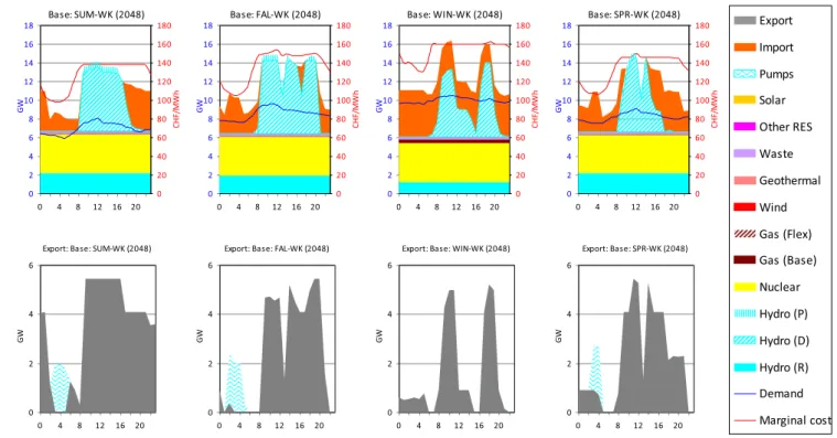
The weekday hourly electricity generation schedule in the Base scenario in each of the four seasons in 2050 is shown in Fig. 9. Electricity exports and energy used for water pumping (for storage) are shown in separate plots. The demand is represented by the blue line and the red line shows the marginal cost of electricity supply in CHF per megawatt hour on the right-hand axis. In the Base scenario in 2050, the total installed capacity is 18.2 GW (Fig. 8) excluding the interconnectors. Three base-load technolo-gies, namely nuclear, run-of-river hydro and gas combined cycle, have a combined capacity of 10 GW, of which 6.6 GW is used for generation in summer (Fig. 9a). The lowest and the highest demands during summer weekdays are 5.9 and 8.1 GW, respectively (Fig. 9a). The supplies 7
From our extensive scenario analyses [33], we found that the highly fluctuating demands in Switzerland (requiring around 3.5 GW of flexible power plants) are easily managed by the availability of large dam and pumped hydro storage facilities. In addition, the interconnec-tors also serve as additional sources of supply (import) and most importantly load dumping (export).
8Years specified in the figures represent the mid-year of periods, i.e. 2020 represents 2018–22; 2048: 2041–55; 2080: 2071–2090. In the legends, Gas (Base) and Gas (Flex) refer to base load and dispatchable gas plants. Electricity consumed by pumped storage plant is shown as Pumps.
from the base-load plants are nearly adequate to meet the demand (blue line) during much of the night time. Never-theless the model imports cheap night time electricity which is stored via pumped hydro (shown in wavy blue pattern in the export graph). When the demand begins to increases from 7 am, electricity generation from dam hydro and pumped hydro commences. Thus the total supply peaks to about 14 GW (vs. the peak demand of 8.1 GW). The excess generation is exported since the export prices are high during the daytime. Electricity import and export occur at the same time, e.g. 6–10 pm, which is to exploit the price difference across the bordering countries. The hourly mar-ginal cost of electricity during the daytime is about 140 and 100 CHF/MWh during the night time.
On winter weekdays (Fig.9c) the availability of run-of-river hydro declines to 1.26 GW (vs. 2.2 GW in summer). About 400 MW of seasonal base-load gas plant is scheduled
to meet high winter demand. It can be seen that this gas plant is not scheduled in other seasons. The total supply from all base-load plants contributes 6.1 GW. However, the lowest demand on the winter weekday is 9.5 GW and demand peaks at 10.5 GW. The gap is filled with imports of cheap electricity during night time and the use of flexible dam hydro for daytime demand. This minimises the import of expensive electricity during the daytime when prices are high. A small quantity of electricity is also exported during morning and evening peaks to profit from the high export price. The marginal cost of electricity varies between 130 and 160 CHF/MWh.
In the other two seasons, spring and fall, the electricity schedule is similar to that of the summer and winter week-days. In summer and fall, overall availability of hydro is high, allowing a larger quantity of exports. In winter and spring, the output from hydro is lower, particularly dam
Installed Capacity 0 5 10 15 20 25 30 2010 2020 2048 2080 2020 2048 2080 2020 2048 2080 2020 2048 2080
BASE BASE-A Hyp Hyp-A
GW
Wood Waste & Biogas Wind Solar Geothermal Oil Gas (Flex) Gas (Base) Nuclear Hydro (P) Hydro (D) Hydro (R) Electricity generation mix
-50 0 50 100 150 200 250 300 350 2010 2020 2048 2080 2020 2048 2080 2020 2048 2080 2020 2048 2080
BASE BASE-A Hyp Hyp-A
PJ
Pumps Wood Waste & Biogas Wind Solar Geothermal Oil Gas (Flex) Gas (Base) Nuclear Hydro (P) Hydro (D) Hydro (R) Fig. 8 Electricity generation
hydro, requiring a larger contribution from imports. The electricity trade option (both import and export) and dam hydro enables the model to balance the supply and demand cost-effectively.
Although electricity imports are balanced with exports on an annual basis as required by the self-sufficiency constraint (refer to Section4.1.1), there is a large seasonal and diurnal variation in trade volume. The generation schedules provide powerful insights into the most cost-effective patterns of electricity trade. Generally about 40 % of electricity export activity occurs in summer while 40 % of the import activity occurs in winter. The large volume of exports in summer is driven by high outputs from hydro and a low demand. In contrast, hydro output declines in winter when the demand is high. Thus, the winter supply gap is met with imported electricity. The dam and pumped hydro (and seasonal base-load gas) plants provide an attractive means to manage the seasonal and daily variations in supply and demand.
Figure10shows the electricity generation schedule of the Base-A scenario from the aggregated model. Similar to the hourly model, the system is optimised to export in summer and import in winter. The dam hydro is scheduled for daytime supply in all seasons. One noticeable difference from the hourly model is the role of pumped hydro storage. Since there is no adequate price incentive to trade, i.e. importing off-peak electricity and exporting during peak, investment in pumped hydro is not cost-effective. Thus, the total electricity trade volume in the aggregated model is about 65 % less than in the hourly model. A combination
of low demand fluctuations and a high contribution from base-load plants means that the marginal cost of electricity varies less than in the hourly model.
Another major reason for choosing a high share of base-load plant in the aggregated model is due to absence of any variation between the weekdays and weekends. The varia-tion in demand between weekends and weekdays is signif-icant (Fig.6), and larger than the variation within individual days. This imposes limits on the role of large base-load capacity—otherwise a large storage or load dumping option is needed for weekends. Figure 11 shows the electricity generation schedule from the hourly model on winter and summer Sundays. Compared to the weekday generation schedule (Fig.9), the weekend schedules vary significantly. While the base-load generation remains the same as on the weekdays, the schedule of non base-load plants and import patterns differ. The demand on Sundays is (relatively) high during evening hours and thus the generation from dam hydro is skewed towards the evening hours. Because of the lower demand on weekends and excess generation from the base-load plants, the marginal cost of electricity is 30– 70 CHF/MWh lower than on the weekdays.
4.3.2 Hyp Scenarios
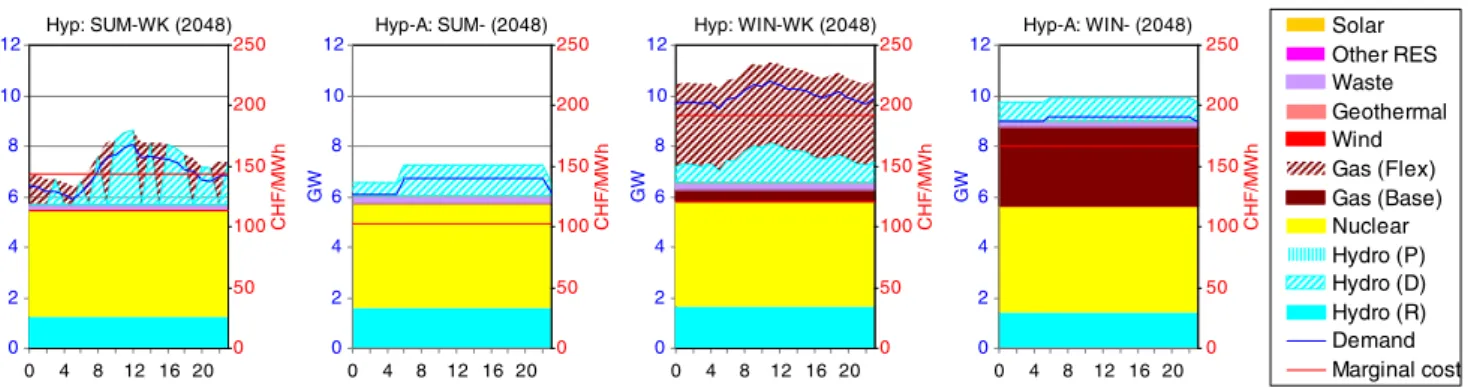
Figure12shows electricity schedule from the Hyp and Hyp-A scenarios in 2050 for summer and winter seasons. Like in the Base scenario, the hourly model deploys a large capacity of flexible gas plant, whereas the aggregated model chooses
a large deployment of base-load gas generation. The total capacity of base-load plants in 2050 is 10.8 GW in the hourly model compared to 14 GW in the aggregated model.
The installed capacity of base-load run-of-river hydro plant in the aggregated model is marginally higher than in the hourly model (1.23 GW in the Hyp scenario vs. 1.57 in
Fig. 10 Electricity schedule in Base-A scenario
Base: SUM-SU (2048) 0 2 4 6 8 10 12 14 16 18 0 4 8 12 16 20 GW 0 20 40 60 80 100 120 140 160 180 CHF /M W h
Export: Base: SUM-SU (2048)
0 2 4 6 0 4 8 12 16 20 GW Base: WIN-SU (2048) 0 2 4 6 8 10 12 14 16 18 0 4 8 12 16 20 GW 0 20 40 60 80 100 120 140 160 180 CHF /M W h
Export: Base: WIN-SU (2048)
0 2 4 6 0 4 8 12 16 20 GW Export Import Pumps Solar Other RES Waste Geothermal Wind Gas (Flex) Gas (Base) Nuclear Hydro (P) Hydro (D) Hydro (R) Demand Marginal cost Fig. 11 Weekend electricity
Hyp-A scenario). The dynamic load curve in the hourly model is managed with some of the existing dam hydro and new investments in dispatchable gas combined cycle plant, whereas the aggregated model can easily supply the smaller variation in demand with base-load gas plant and existing dam hydro plants.
In winter, the large variation in demands is managed in the hourly model with flexible dam and gas power plants. The flexible gas plants are scheduled only during winter weekdays and therefore have a low utilisation rate. This in turn incurs a high system cost (Fig.14).
The hourly model also provides powerful insights in the period 2080 when solar PV is deployed. In 2080, a relatively large capacity of solar PV is chosen in the hourly model (Fig.8). Figure 13shows the generation schedule in 2080 for the Hyp scenario from both models. Electricity
generation from solar PV begins at 5 am, coinciding with an increase in demand. The combined supplies from the base-load and solar PV plants exceed the demand and the excess electricity is stored via pumped hydro facilities. The stored electricity is discharged in the evening when the solar PV output begins to decline. Since the supply is more than demand, and there is no option for export, the marginal cost declines drastically during daytime compared to the night time. A similar trend is also seen in winter despite the high demand and relatively low output from solar PV. The large investment in solar PV in the hourly model can be attributed to its bell-shaped daytime output pattern (Fig. 7), which coincides with daytime demands (and high export prices in the Base scenario).
On weekends, however, the solar PV is not used because outputs from the base-load are fully adequate to meet the Hyp: SUM-WK (2048) 0 2 4 6 8 10 12 0 4 8 12 16 20 GW 0 50 100 150 200 250 CHF /M W h Hyp-A: SUM- (2048) 0 2 4 6 8 10 12 0 4 8 12 16 20 GW 0 50 100 150 200 250 C H F/ M W h Hyp: WIN-WK (2048) 0 2 4 6 8 10 12 0 4 8 12 16 20 GW 0 50 100 150 200 250 CHF /M W h Hyp-A: WIN- (2048) 0 2 4 6 8 10 12 0 4 8 12 16 20 GW 0 50 100 150 200 250 C H F/ M W h Solar Other RES Waste Geothermal Wind Gas (Flex) Gas (Base) Nuclear Hydro (P) Hydro (D) Hydro (R) Demand Marginal cost Fig. 12 Electricity generation schedule in Hyp and Hyp-A scenarios in 2050
Hyp: SUM-WK (2080) 0 2 4 6 8 10 12 14 0 4 8 12 16 20 GW 0 50 100 150 200 250 C H F/ M W h
Export: Hyp: SUM-WK (2080)
0 1 2 0 4 8 12 16 20 GW Hyp-A: SUM- (2080) 0 2 4 6 8 10 12 14 0 4 8 12 16 20 GW 0 50 100 150 200 250 CHF /M W h
Export: Hyp-A: SUM- (2080)
0 1 2 0 4 8 12 16 20 GW Hyp: WIN-WK (2080) 0 2 4 6 8 10 12 14 0 4 8 12 16 20 GW 0 50 100 150 200 250 CHF /M W h
Export: Hyp: WIN-WK (2080)
0 1 2 0 4 8 12 16 20 GW Hyp-A: WIN- (2080) 0 2 4 6 8 10 12 14 0 4 8 12 16 20 GW 0 50 100 150 200 250 CHF /M W h
Export: Hyp-A: WIN- (2080)
0 1 2 0 4 8 12 16 20 GW Export Import Pumps Solar Other RES Waste Geothermal Wind Gas (Flex) Gas (Base) Nuclear Hydro (P) Hydro (D) Hydro (R) Demand Marginal cost
demands. As the result, overall capacity factor (utilisation) of solar PV is low. Nonetheless, solar PV is still cost-effective because its daytime weekday output in both sum-mer and winter is very valuable. Enabling more pumped hydro potential (or a higher availability assumption for pumped hydro) could enhance the utilisation of solar PV on weekends too. Any short-term intermittency of solar PV could be manageable in the Hyp scenario through shifting the timing of flexible dam hydro or gas generation, assum-ing the average total output from solar PV over the season is maintained.
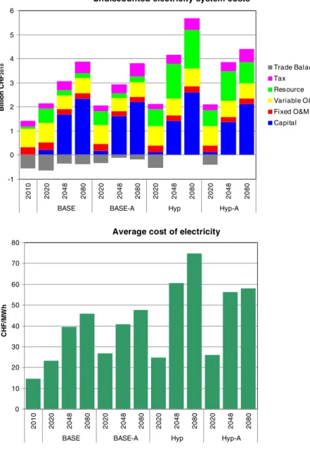
4.4 System Costs
Annual undiscounted electricity system costs and average electricity costs from both models are shown in Fig.14. The trade balance (shown in grey shading) refers to the net cost/
profit from electricity trade. Though the net volume of trade is set to zero through the self-sufficiency constraint, the revenue from trade is attributable to the price difference between imports and exports across trading partners and timeslices. As seen before, the electricity trade volume in the hourly model (Base scenario) is high and therefore there is a large positive trade balance (profits) in the Base scenar-io. Because of this trade profit, the average cost of electricity is slightly lower in the hourly model compared to the ag-gregated model (Base-A scenario). The overall difference in annual undiscounted system cost between the two scenarios is less than 5 %.
In the Hyp scenarios, the cost differs significantly be-tween the two models. In 2050, the undiscounted system cost is 8 % higher in the hourly model compared to the aggregated model, and the difference increases to 22 % in 2080. In the Hyp scenario, resource cost is significantly
Undiscounted electricity system costs
-1 0 1 2 3 4 5 6 2010 2020 2048 2080 2020 2048 2080 2020 2048 2080 2020 2048 2080
BASE BASE-A Hyp Hyp-A
B illio n C H F 2010 Trade Balance Tax Resource Variable O&M Fixed O&M Capital
Average cost of electricity
0 10 20 30 40 50 60 70 80 2010 2020 2048 2080 2020 2048 2080 2020 2048 2080 2020 2048 2080
BASE BASE-A Hyp Hyp-A
C H F/ M W h
Fig. 14 Undiscounted system costs and unit cost of electricity
higher than in the Hyp-A scenario because the hourly model chooses flexible gas plant with relatively low efficiency. The aggregated model deploys efficient base-load gas plants, requiring less natural gas. This higher system cost in the hourly model is also attributable to the need for additional installed capacity (see Fig. 8) to manage the higher peak compared to the aggregated model. Some of this capacity, particularly solar PV and flexible gas plants, is underutilised during weekends and summers, respectively, leading to the higher electricity cost in the hourly model (Hyp scenario).
5 Discussion
The results presented above illustrate a number of similari-ties between the hourly and aggregated modelling approaches, along with some important differences. Even though both the hourly and aggregated models give fairly similar results for the conventional Swiss electricity system (Base scenario), this comparative analysis reveals signifi-cant differences between the models for the more general-ised Hyp scenarios. The similarity in the Base scenario solutions arises because the Swiss energy system is endowed with plenty of dispatchable dam hydro resources, storage options (pumped hydro) and trade options (in effect amounting to load dumping options) to manage supply and demand. While many other countries possess some flexible dam hydro resources and participate in trading, both are generally on a much smaller scale relative to total demand than in Switzerland. Thus, the insights from the Hyp scenar-ios may be more relevant when considering different levels of temporal detail for modelling a broader range of countries.
Some of the key differences observed between the two modelling approaches in the more generalised Hyp scenario relate to the deployment and utilisation of renewables, flex-ible gas-fired generation and storage. For instance, intermit-tent solar PV technology represents an attractive option in the hourly model to supply high daytime peak demand, in conjunction with pumped hydro storage. In the aggregated model, solar PV is much less attractive because the aggre-gation reduces the overall demand peak and the output peak for solar capacity. Similarly, the large difference between peak and base-load demands (or between weekday and weekend demands) represented in the hourly model sup-ports flexible (dispatchable) gas-fired generation, whereas the aggregated model can rely to a large extent on base-load technologies. In sum, the aggregated model tends to over-estimate the potential contribution of large base-load power plants and underestimate the need for supply–demand man-agement and storage. Thus, there appears to be a significant value added by the higher inter-temporal resolution avail-able in the TIMES framework, in providing an enhanced
representation of load balancing in the electricity system. This is important for the application of these models in supporting policy and other decision makers explore differ-ent strategies for the long-term developmdiffer-ent of the electric-ity system.
5.1 TIMES Versus Traditional Dispatch Models
It is evident that the hourly model provides powerful insights into the generation schedule. However, the TIMES framework cannot necessarily account for reliability and stochastic characteristics of the electricity system, or prob-able unserved energy or loads, which are typically repre-sented in electricity dispatch models [26]. For example, in TIMES framework, technology is assumed to be available on average throughout the year up to its availability factor. However, in real-world operation some generation capacity may be completely unavailable during outages. Therefore there are possibilities for unserved loads when the electricity system has a limited number of large base-load plants. This can be partly addressed in the TIMES framework by requir-ing high reserve margins aimed to cope with such outages. As an area for future analysis, the generation schedule from the hourly STEM-E can be validated with a dispatch model to assess the divergence from real-world operation. One validation approach would be to implement the tech-nology mix and generation mix as the input to a dispatch model and run the dispatch model in ‘operational’ mode. Such a validation would provide additional results on power system-specific parameters like demand unserved, loss of load probability and so on. A similar methodology was adopted to test the reliability of the electricity sector from the UK MARKAL model (with six timeslices) by soft link-ing the UK MARKAL model to the Wien Automatic Sys-tem Planning (WASP) model—an electricity generation expansion plan model [13].
5.2 System Versus Sectoral Approaches
Although the TIMES framework does not account for some features available in dispatch models, its integrated system approach may be complementary. For example, dispatch models represent the electricity sector only and are generally static in terms of generation stock. Thus, they are less suitable for analysing dynamics and emerging energy sys-tem developments in other sectors that affect the electricity sector. For example, electric mobility may provide a decar-bonisation pathway for the transport sector. However, the impact of electric and plug-in vehicles on the electric net-work (demand) cannot be analysed with dispatch models without assumptions on charging behaviour. For such a complex system development, TIMES’s energy system ap-proach is powerful because it endogenizes key system
characteristics such as the electricity load curve. Although the TIMES models presented here cover only the electricity sector, we are exploring options to include a high level of temporal detail in a TIMES model of the whole energy system [47]. A plug-in modular approach has been envis-aged so that the same model can be used as a stand-alone electricity model for power sector analyses and system model for energy policy analysis, if the computational com-plexity to be addressed.
5.3 Demanding Input Data Requirements
Clearly, the high inter-temporal resolution in STEM-E is demanding in terms of data requirements. Such a model requires hourly data for inputs such as the historical perfor-mance of existing technologies, the load curve for end-use sectors (and technologies), resource availability and others, which are often not available. There are thus trade-offs between the incremental insights provided by a high level of time resolution and the demanding resources to develop and solve such a model (e.g. input data and computational facilities). Despite the good availability of data for Switzer-land, we nonetheless had to make a number of assumptions and approximations where data were not available. For other countries, or for an even higher level of temporal resolution, the number of assumptions or approximation may under-mine the reliability of the detailed inter-temporal model. Therefore, the availability of input data is one of the key determinants in choosing the number of timeslices. If the data availability is poor or subject to high future uncertainty, an aggregated model could be a more suitable choice. Again, the choice of timeslices also depends on the energy system in question, and the policy and research applications of interest. For some applications, an aggregated model can still provide some robust insights as seen from the Base scenarios analyses.
5.4 Computational Complexity
The large number of timeslices considerably increases com-putational resource requirements. We compared computa-tional resource usage from both models, solved with the CPLEX solver on a quad processor machine9 using four threads (Table4). Importantly, STEM-E is formulated as a mixed integer model to account for the minimum scale of nuclear generation plant (so-called ‘lumpy’ investment). Because mixed integer programming (MIP) problems are solved using heuristics, the solution time and resource usage of different model runs is not necessarily comparable. Ac-cordingly, Table 4 also reports linear programming (LP) versions of the Base and Base-A scenario. The LP versions
of the Base scenario solved in 506 s compared to less than a second for the Base-A scenario. The MIP solution times were in roughly the same ratio.
The hourly model comprises a much larger number of equations (around 25 times larger), and thus requires exten-sive resources. The Hyp scenario solved with one fourth of the time used in the Base scenario, indicating that the optimization of hourly electricity trade in the Base scenario is resource intensive. Despite the fact that the Swiss electricity system is small, the size of the hourly model is twice the size of our Global Multi-regional MARKAL (GMM) model [27]. We should also mention that attempts to incorporate lumpy in-vestment in STEM-E for additional technologies (i.e. increas-ing the number of integer variables in the MIP problem) was computationally challenging. Therefore, introducing high number of timeslices in large energy or electricity system model requires careful choice of timeslices and the use of an appropriate solver algorithm, and involves trade-offs in terms of representing other features such as lumpy investment or endogenous technology learning.
5.5 Alternatives
To address the computational and data availability issues, a number of alternatives are possible to approximate some elements of a more detailed load curve in a conventional energy system model to improve electricity sector depiction. Most of these involve diverging from conventional approaches of defining inter-temporal timeslices based on traditional seasonal classification or electricity tariff-based definitions of day and night. Instead, timeslicing should be based on real data on inter-temporal variations in the elec-tricity demand (load) curve; availability of energy resource supply options; and the research question to be answered. There is no rule of thumb in timeslicing, but the following are some guidelines.
& If a specific domestic resource is seen as the key elec-tricity supply option (e.g. hydro, solar and wind), or if there is a strong policy interest on a specific technology or resource (e.g. feed-in tariff), then the choice of time-slices could be based on characteristics of the technolo-gy/resource in question so that their operational characteristic can be realistically modelled.
& When the number of intra-annual timeslice is small, this leads to an averaging of capacity demands and thus underestimates the real demand peak (e.g. as seen in Fig. 7). This can be partly addressed by defining the timeslices in a way that ensures a better representation of the peak, such as with:
& An uneven seasonal time split to capture some of the seasonal variations in demand and/or resource 9
supply. For example, a timeslice could be defined to represent one peak winter ‘month’ rather than the full winter season of 3 or 4 months.
& A non-uniform diurnal time split. For example, a time split that defines‘day’ according to the peaking hours in each season could be chosen, or according to daylight hours if solar PV has a significant poten-tial. In this case, annual time fractions and demand fractions need to be disaggregated appropriately. & An alternative to ensure the impact of large variations in
demand is represented in the choice of base-load and dispatchable generation technology, is to introduce a share constraint for base-load and dispatchable technologies. This could be determined from the highest and lowest electricity demand hours in each season. However, any such a constraint could have negative implications for future years, particularly for a full energy system model. & Similarly, a non-conventional electricity reserve margin
could be applied based on the differences between the average capacity demand and hourly peak demand (also see [35, 38]). This reserve margin would need to be larger than prevailing rule of thumb values used by electric utilities to cover the instantaneous peak and spinning reserves. However, while this approach may ensure a more appropriate representation of total capac-ity requirements, it does not represent generation and dispatch at the peak.
& In some countries, weekly (weekdays vs. weekends) demand variations are more significant than seasonal variation (e.g. in tropical countries). Unlike the seasonal demand variations, the weekly variation implies addi-tional limitations on the operation of large base-load plants (operational control in case of nuclear plants and large efficiency penalty for fossil fuel plants). In such cases, a time split can be applied at the weekly level. For
example, in many tropical countries lighting and cooling are major energy service demands which do not vary significantly across seasons. In such case, a seasonal split can be replaced with a weekday–weekend split. For example, in the Singapore MARKAL model [12] weekdays, Saturday and Sunday were used instead of a conventional seasonal split.
6 Conclusions
We used the bottom-up TIMES modelling framework to develop a model of the Swiss electricity system combining detailed technology pathways, an hourly load curve and a long model horizon. The high level of inter-temporal detail in this model provided richer insights into the operational schedule of power plants and marginal electricity production costs at the hourly level. Despite the computational and data intensity of this model, the results of a number of scenario analyses demonstrated that hourly resolution leads to a far better solu-tion than an equivalent aggregated inter-temporal model. Therefore, there are considerable benefits in investing in data collection and exploiting developments in computational and solver power. There is no rule of thumb for inter-temporal timeslicing. The ideal number of timeslices to represent in a model depends on energy system characteristics, the research question to be answered and, most importantly, the availability of data at the timeslice level. Some approaches suggested in the discussion could be considered while developing new modelling tools. Insofar as an hourly TIMES model can represent some of the features of electricity dispatch, it cannot fully replace an electricity dispatch model because the TIMES framework does not account for reliability and stochastic characteristic of technologies. However, the TIMES frame-work’s integrated system approach and long model horizon are complementary to dispatch modelling.
Table 4 Computational resource usage in both models
Scenarios Single equations Single variables Non-zero elements Resource usage (s) Iteration count
Base (LP) 268,227 209,495 1,658,365 506 61,029 Base-A (LP) 10,660 9,001 57,474 0.91 4,602 Base 268,257 209,630 1,658,650 873 72,790 Base-A 10,690 9,136 57,759 2 7,844 Hyp 263,250 205,011 1,572,742 224 18,548 Hyp-A 10,482 8,992 55,181 1.16 5,768 GMM Ref (LP) 97,514 81,738 560,657 68 4,332 GMM Ref (ETL) 105,219 85,858 602,296 39,565 5,043,460
GMM Global Multi-regional MARKAL energy system model, LP Linear programming, ETL Endogenous Technology Learning using MIP formation
All scenarios are solved in a dual core machine (Intel Core2 Quad Q9400 @ 2.66 GHz and 3 GB RAM) using the following CPLEX12.2 (GAMS 23.5.2) solver parameters: iis yes, lpmethod 1, baralg 1, barcrossalg 1, barorder 2, threads 4 (others default)
Acknowledgments Earlier versions of this paper were presented at the ETSAP Workshop held in New Delhi and Stockholm [36,37]. The author thank many people, who offered their support during the devel-opment of this model, particularly addressing the computational and solver issues, MIP formulation and fixing the storage algorithms. This paper is partly conceptualised based on the review comments from an earlier publication [38] and the contribution from the reviewers is highly appreciated.
References
1. ADAM (2010). Adaptation and mitigation strategies: supporting European climate policy, Tyndall Centre.http://www.tyndall.ac.uk/ adamproject/about. Accessed Sept 2012.
2. Atukeren, E., Lassmann, A., Abrahamsen, Y. (2008). Switzerland’s electricity trade: a short-term forecasting model and an analysis of multivariate relationships, EEM (pp. 1–6). 5th International Con-ference on European. doi:10.1109/EEM.2008.4579018.
3. Bahn, O., & Frei, C., (2000). GEM-E3 Switzerland: a computable general equilibrium model applied for Switzerland, PSI Bericht No. 00-01. Paul Scherrer Institute: Villigen.http://eem.web.psi.ch/ Publications/Other_Reports/PSI_00-01.pdf.
4. Bernard, A., Vielle, M., Viguier, L. (2005). Carbon tax and inter-national emissions trading: a Swiss perspective. In A. Haurie, L. Viguier (Eds.), Coupling climate and economic dynamics (pp. 295–319). New York: Kluwer.
5. BFE (2000–2010). Schweizerische Elektrizitätsstatistik, Bundesamt für Energie, Bern. http://www.bfe.admin.ch/themen/00526/00541/ 00542/00631/index.html?lang0de&dossier_id000765.
6. BFE (2000–2010). Schweizerische Gesamtenergiestatistik, Bunde-samt für Energie, Bern; various publication 2000–2009. http:// w w w. bf e . a dm i n. c h / t he m en / 0 0 52 6 / 0 0 54 1 / 0 05 4 2 / 0 06 3 1/ index.html?lang0de&dossier_id000763.
7. BFE. (2007). Die Energieperspektiven 2035. Bern: Bundesamt für Energie.
8. BFE (2010). Stilllegungsfonds für Kernanlagen & Entsorgungs-fonds für Kernkraftwerke - Faktenblatt Nr. 1: Rechtsgrundlagen, Organisation und allgemeine Informationen, Bundesamt für Ener-gie, Bern. http://www.news.admin.ch/NSBSubscriber/message/ attachments/20511.pdf.
9. Blesl, M. (2008). TIMES Pan European Model (TIMES-PEM of NEEDS). http://www.etsap.org/Applications/NEEDS-TIMES-PEM-summary-MB.pdf.
10. Boqiang, R., & Chuanwen, J. (2009). A review on the economic dispatch and risk management considering wind power in the power market. Renewable and Sustainable Energy Reviews, 13, 2169–2174.
11. Bretschger, L., Ramer, R., Schwark, F. (2009). How rich is the 2000 Watt Society? Impact of energy conservation policy Measures on innovation, investment and long-term development of the Swiss Economy, Swiss Federal Institute of Technology. http://www.cer .ethz.ch/resec/people/rramer/Brochure_2kW.pdf.
12. Chang, Y., Ho, H. K., Leong, K. C., Osman, R., Toh, K. C., Chen, Y., Kannan, R. (2006). Final report on the economics of the Kyoto Protocol: a cost-benefit analysis for Singapore. Singapore: Minis-try of Trade and IndusMinis-try.
13. Chaudry, M., Dougamas, A., Ekins, P., Kannan R, Shakoor A, Skea J, Strbac G, Wang X. (2009). A resilient UK Energy system: building in resilience, UKERC Research Report.http://www.ukerc.ac.uk/support/ tiki-download_file.php?fileId0618.
14. Connolly, D., Lund, H., Mathiesen, B. V., Leahy, M. (2010). A review of computer tools for analysing the integration of renewable energy into energy systems. Applied Energy, 87, 1059–1082.
15. Econability (2010). GENESWIS computable general equilibri-um model for Switzerland. http://www.econability.com/ models.htm.
16. Ecoplan (2006). Branchenszenarien Schweiz: Langfristszenarien zur Entwicklung der Wirtschaftsbranchen mit einem rekursiv-dynamischen Gleichgewichtsmodell (SWISSGEM). http:// www.ecoplan.ch.
17. Ecoplan (2006). Zukunfts- und wachstumsorientiertes Steuersys-tem (ZUWACHS).http://www.ecoplan.ch.
18. Ecoplan (2008). Volkswirtschaftliche Auswirkungen von CO2-Abgaben und Emissionshandel für das Jahr 2020.http://www.e coplan.ch/download/co2g_sb_de.pdf.
19. EEX–European Electricity Exchange. Market Data (2008).http:// www.eex.com/en/Market%20Data. Accessed 15 August 2010. 20. ENTSO–European Network of Transmission System Operators for
Electricity (2010).https://www.entsoe.eu/resources/data-portal/. 21. ETEM (2011). Energy technology environment model. http://
apps.ordecsys.com/etem.
22. ETS–Der Energie Trialog Schweiz (2009). Energie-Strategie 2050 —Impulse für die schweizerische Energiepolitik. Grundlagenber-icht.http://www.energietrialog.ch/cm_data/Grundlagenbericht.pdf. 23. ETSAP (2008). Categories of models and applications. http://
www.etsap.org/Models&applicationsMainPage.asp.
24. EWI (2010). Dispatch and investment model for electricity markets in Europe, The Institute of Energy Economics, University of Cologne. http://www.ewi.uni-koeln.de/fileadmin/user/PDFs/ DIME_Model_description_.pdf.
25. Foley, A. M., Gallachóir, B. P. Ó., Hur, J., Baldick, R., McKeogh, E. J. (2010). A strategic review of electricity systems models. Energy, 35(12), 4522–4530.
26. Garcés, F. F. (2004) Electric power: transmission and generation reliability and adequacy. Encyclopaedia of Energy, 301–308 27. Gül, T., Kypreos, S., Turton, H., Barreto, L. (2009). An
energy-economics scenario analysis of alternative fuels for transport using the global multi-regional MARKAL Model GMM. Energy, 34(10), 1423–1437.
28. Howells, M., et al. (2011). OSeMOSYS: the open source energy modeling system. Energy Policy. doi:10.1016/j.enpol.2011.06.033. 29. Hirschberg, S., Bauer, C., Burgherr, P., Biollaz, S., Durisch, W., Foskolos, K., et al. (2005). Neue Erneuerbare Energien und neue Nuklearanlagen: Potenziale und Kosten. PSI-Report no.05-04. Paul Scherrer Institut, Villigen PSI, Switzerland.http://gabe.web. psi.ch/pdfs/PSI_Report/PSI-Bericht_05-04sc.pdf.
30. Jakob, M. (2007). The drivers of and barriers to energy efficiency in renovation decisions of single-family home-owners, Center for Energy Policy and Economics CEPE, Department of Management, Technology and Economics, ETH Zur-ich.http://www.cepe.ethz.ch/publications/workingPapers/CEPE_ WP56.pdf.
31. Johnsson, F. (2011). Methods and models used in the project used in the project pathways to sustainable european energy systems, Alli-ance for Global Sustainability.http://www.energy-pathways.org/pdf/ Metod_reportJan2011.pdf.
32. JRC–Joint Research Centre (2009). Photovoltaic geographical in-formation system (PVGIS): geographical assessment of solar re-source and performance of photovoltaic technology. http:// re.jrc.ec.europa.eu/pvgis/apps4/pvest.php. September 2009. 33. Kannan, R., & Turton, H. (2012). Cost of ad-hoc nuclear policy
uncertainties in the evolution of the Swiss electricity system, Energy Policy. Doi: 10.1016/j.enpol.2012.07.035.
34. Kannan, R., & Turton, H. (2011). Documentation on the develop-ment of Swiss TIMES electricity model (STEM-E). Switzerland: Paul Scherrer Institut.
35. Kannan, R. (2009). Uncertainties in key low carbon power gener-ation technologies—Implication for UK decarbonisation targets. Applied Energy, 86(10), 1873–1886.
![Fig. 3 Temporal depiction tree in STEM-E. Modified from Remme and Blesl [52]](https://thumb-eu.123doks.com/thumbv2/123doknet/14872492.640548/5.892.277.812.731.1072/fig-temporal-depiction-tree-stem-modified-remme-blesl.webp)