Special Issue Honouring Helias A. Udo de Haes: LCA Methodology
Continent-specific Intake Fractions and Characterization Factors for
Toxic Emissions: Does it make a Difference?
David Rochat1, Manuele Margni 2,1 and Olivier Jolliet 3,1*
1Life Cycle Systems, GECOS, Institute of Environmental Science and Technology, Ecole Polytechnique Fédérale de Lausanne, Section 2,
1015 Lausanne EPFL, Switzerland
2CIRAIG, Ecole Polytechnique de Montreal, C.P. 6079, Succursale Centre Ville, Montreal (Qc) Canada, H3C 3A7 3Center for Risk Science and Communication, Department of Environmental Health Sciences, School of Public Health,
University of Michigan, Ann Arbor, MI 48109, USA
* Corresponding author ([email protected])
Introduction
The development of generic characterization factors (CF) in life cycle impact assessment (LCIA) is historically motivated by the lack of spatial and temporal information when deter-mining the environmental interventions per functional unit. These generic characterization factors are well adapted to evaluate global impacts, such as global warming and ozone layer depletion, but face criticisms when assessing all those impact categories that are not global in nature such as acidi-fication, eutrophication, toxicity, etc. From a scientific point of view, one of the major problems is the inability to ad-equately model impacts due to a common disregard of the spatial differences in the fate and exposure and in the effect of environmental stressors (Udo de Haes et al. 2002). From a practical point of view, accounting for spatial differentia-tion in LCA remains complicated by the lack of spatial dis-tinction maintained in most emissions and resource consump-tion inventory databases. However, there is an increasing demand on impact assessment methodologies reflecting re-gional concerns and being adapted to the local conditions for such impact that are not global in nature. It is not sur-prising having practitioners being reluctant applying char-acterization factors developed for a European context to assess impacts of toxic emissions related to another conti-nent. This paper therefore aims to develop characterization factors for toxic air emissions in different continents and to analyze under which conditions this spatial distinction makes a significant difference compared to generic characteriza-tion factors. In addicharacteriza-tion, adapting LCIA methods to devel-oping countries is one of the most important needs and ob-jectives of the Life Cycle Initiative (Jolliet et al. 2004, Stewart and Jolliet 2004).
Several publications have quantified the variability linked to spatial inhomogeneity in multimedia modeling at national or regional scale (Klepper and den Hollander 1999, McKone et al. 2001, MacLeod et al. 2001, MacLeod et al. 2004, Prevedouros et al. 2004, Pennington et al. 2005, Wegener Sleeswijk 2005). Disregarding the release location, results demonstrated likely variations of up to two or three orders of magnitude in the chemical concentrations and human intake fractions, particularly for emissions to water. The variability linked to the release location could even increase up to 6 orders of magnitude (MacLeod et al. 2004, Penning-ton et al. 2005). Based on such findings, MacLeod et al.
DOI: http://dx.doi.org/10.1065/lca2006.04.012 Abstract
Goal and Scope. This paper aims to develop continental
charac-terization factors for the human toxicity impacts of emissions released to air in different continents and to analyze under which conditions this spatial distinction makes a significant difference compared to generic characterization factors.
Methods. The IMPACT 2002 multimedia and multipathways
model has been parameterized to define 6 continental box-mod-els, each of them nested in a world box in order to capture impacts of emissions leaving the initial continent. Applying the model to a test set of 31 heterogeneous chemicals emitted to air, intake fractions and human toxicity characterization factors were calculated for each continent and compared.
Results and Discussion. For a given chemical, characterization
factors can vary of typically a factor 5 to 10 between continents (max 102), mainly as a function of population density for
inha-lation and as a function of the total agriculture production per km2 for ingestion. This is significant but still limited compared
to the variation between substances, of 106 in intake fraction
and of 1012 in cumulative risks.
Conclusion. The variation amplitude is limited for persistent
chemicals and decreases with the fraction of the chemical advected out of the continent. Moreover, the ranking between continents remains almost the same for all chemicals. Therefore generic characterization factor for air emissions calculated at continental level, such as the one proposed by the common life cycle assessment method, are in most cases suitable for com-parative purposes in any other continent. However, continent specific characterization factors are required if one is interested in evaluating absolute values or in comparing impact between scenarios with emissions in very different continents. For this purpose, a simplified but accurate correlation is determined to extrapolate continent specific intake fractions and characteri-zation factors of a wide range of substances for Oceania, Af-rica, South AmeAf-rica, North America and Asia, starting from the results of Europe as a base continent.
Recommandation and Perspectives. Further research should
fo-cus on linking the different continental boxes to obtain a global spatial model including major climatic phenomenon such as the air transport by jet stream. The level of spatial resolution, how-ever, has to be carefully selected to capture significant differ-ences, but at the same time to avoid unnecessarily requirement efforts for data gathering and calculation capabilities.
Keywords: Continent-specific variation; human toxicity; intake fraction; life cycle assessment (LCA); toxic emissions
(2004) provided 4 chemical specific regressions to extrapo-late exposure estimates from the population density and the food production intensity variables. These correlations are however substance specific and cannot be used for extrapo-lation purposes across a wide range of substances.
All these works were focusing on a spatial differentiation with reference to zones of about 5 to 10 hundreds square kilometers. Characterization factors for human toxicity, HDF, at continental level have mainly been published for US (Hertwich et al. 2001), for Europe (Goedkoop et al. 2000, Huijbregts et al. 2000, Jolliet et al. 2003) and for Japan (Itsubo 2003). Little information is published for other tinents and the existing ones cannot be compared on a con-sistent basis. Huijbregts and co-authors (2003) investigated the uncertainty in fate and exposure factors of different ge-neric continent-specific environments, using a consistent model. They find out this could be moderately high, between a factor 2 to 10. They also propose correlations relating Australia and US to European factors, but without account-ing for the specific chemical properties and parameters that determine if impact is mostly local or global. In addition, the authors claimed for further research to investigate whether the systematic differences found between the dif-ferent evaluative environments are of direct relevance for LCA purposes.
We therefore aim to calculate differentiated intake fractions (iF) and human toxicity characterization factors for differ-ent contindiffer-ents using a consistdiffer-ent model to answer the fol-lowing questions:
• How to model iF and characterization factors for vari-ous continents, taking into account the specific chemical properties?
• What is the data availability and variability at world level for calculating iF?
• How far is the variability of iF and CFs between conti-nents significant? How does it compare to the variations between chemicals?
• What are the environmental and geographical key pa-rameters affecting iF and its variation across continents? • How to derive a general relationship to extrapolate con-tinent-specific iFs and CFs of a wide range of specific chemicals, starting from the modeled intake fraction of a base continent.
We will first introduce the methodology in section 1, pre-senting the selected model, its structure and the data used to parameterize the different continents. In section 2, we will present results for a test set of 31 chemicals and analyze the continental variability in intake fractions as a function of chemical properties. We then propose a simplified but accu-rate method to extrapolate continent-specific iFs and CFs based both on chemical specific properties and on continent specific properties such as population densities. Results are focused on an air emission scenario, as air emissions are the most likely to involve both local impacts and long range transportation. In the conclusion (section 3) we will finally discuss the question contained in this paper title: does it make a difference and under which conditions?
1 Method
1.1 Framework and selection of the model
Characterization factors for toxicological impacts, CF [Im-pact/Mass] are based on models that account for chemical fate in the environment – F [time], human exposure – E [time–1], and differences in toxicological response, as defined by the effect factor – EF [Impact/Mass]. This can be ex-pressed in the following simplified equation (Guinee et al. 1996, Jolliet 1996, Goedkoop et al. 1999, Huijbregts et al. 2000, Hertwich et al. 2001, Udo de Haes et al. 2002):
re i mr i re i nr i mn i me i
F
E
EF
iF
EF
CF
=
⋅
⋅
=
⋅
(1)The intake fraction, iF [dimensionless] combines fate and exposure factors describing the fraction of an emission that is ultimately taken in by a population (Bennett et al. 2002b). Subscript i describes a given chemical, superscripts m the emission compartment, n the environmental compartment,
r the route of exposure and e the effect type (e.g. cancer or
non-cancer). As effect factors in LCA are usually assumed to be additive, linear and independent of the time and loca-tion of exposure, the characterizaloca-tion factor is assumed lin-early proportional to iF.
Among the existing multimedia and multipathways expo-sure models (McKone 1993, Brandes et al. 1996, Huijbregts et al. 2000, MacLeod et al. 2001, Pennington et al. 2005), the authors selected IMPACT 2002 (Pennington et al. 2005) as it is well adapted for studying spatial differentiation. It consists of a common multimedia fate, a multipathways exposure model, and two effect modules for human health and ecotoxicity. IMPACT 2002 enables estimation of chemi-cal concentrations in environmental media at a regional and a global scale. The human multiple pathways exposure mod-ule links chemical concentrations in environmental media (atmosphere, soil, surface water, and vegetation) calculated by the fate model to human intake though inhalation and ingestion. Ingestion pathways include drinking water con-sumption; incidental soil ingestion; and intake of contami-nants in agricultural products (fruits, vegetables, grains,…) as well as in animal products, such as beef-, pig-, and poul-try-meat, eggs, fish, and milk. Intake fractions are calcu-lated from the contaminant concentration in food and live-stock production levels at each location, the water extracted to serve a given population at each location, as well as the population distribution when considering inhalation. The agricultural vegetation module in the chemical fate model IMPACT 2002 distinguishes two major types of vegetation, as suggested by McKone (1993): exposed and unexposed produced. The first one being exposed to atmospheric depo-sition, similar to foliage in the fate module, and the second protected from such direct contact with the atmosphere like stems and comestibles roots.
Cumulative risk and potential impact per kg of emission are calculated by combining cumulative chemical intake with risk-based effect factors. However, a detailed study of hu-man risks remain outside the main scope of the present study, which is mainly focused on fate and exposure.
1.2 Adapting IMPACT 2002 to other continents
Six continental models are developed by adapting the West-ern European model to all continents worldwide. A typical nested approach (Cowan et al. 1994) was adopted with a continental box nested in a world box to account for any intake that may occur as a result of contaminant advection outside of the initially considered continental region. This is in line with the broadness of the LCA approach, accounting for the overall impacts both within and outside the nent of emission. The geographical boundaries of the conti-nental boxes are shown in Fig. 1.
Parameters affecting the fate, the exposure, and thus the human intake fraction were specifically collected for each continent. As a first approximation we decided to modify a selected number of parameters responsible for the highest variations between continents. Geographical data such as surface area, the share of land, fresh water and marine wa-ter, as well as the freshwater mean depth were calculated using Geographic Information System (GIS). Mean annual
precipitation and runoff data (rainfall – evapo-transpiration) were taken from 0.5 x 0.5 degree grid data from the Global Run Off Data Centre (GRDC) (Global Runoff Data Centre 2004). Annual average air flow are calculated using the un-derlying wind velocity data of the model GEOS-CHEM (Bey et al. 2001) and the perpendicular cross-sectional areas, with air sub-divided according to a grid. Population data were taken from the CIA factbook (CIA 2004). In this simplified data gathering procedure, default values of IMPACT 2002 such as soil depth, pH, suspended particulate matter, OH concentration, etc. remained unchanged for all the conti-nents (Pennington et al. 2005) as the impact of their vari-ability is restricted at a continental scale. Table 1 summa-rizes the collected data specific to each continent and de-scribes the corresponding literature sources.
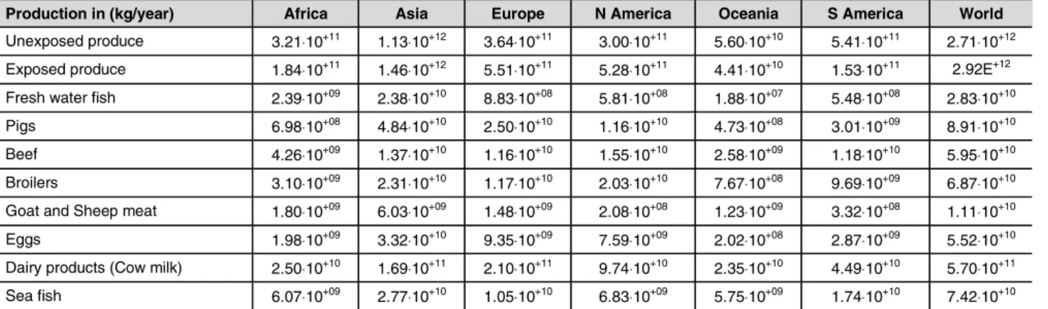
Human exposure via food is linked to the location where the food is produced. Food agricultural production statis-tics were taken from Faostat database (FAO 2004). Food production for each continent is given in Table 2 and summed up to a world production. The model takes into account the
Fig. 1: Areas covered by the continental boxes
Africa Asia Europe N America Oceania S America World Source
Population 7.96⋅10+8 3.76⋅10+09 6.51⋅10+08 4.89⋅10+08 3.10⋅10+07 3.47⋅10+08 6.07⋅10+09 CIA factbook
Soil Area (m²) 3.01⋅10+13 4.63⋅10+13 7.74⋅10+12 2.08⋅10+13 8.07⋅10+12 1.77⋅10+13 1.31⋅10+14 calculated with GIS
Seawater Area (m²) 1.95⋅10+13 5.51⋅10+13 6.49⋅10+12 2.54⋅10+13 2.05⋅10+13 2.56⋅10+13 3.65⋅10+14 calculated with GIS
Freshwater Area (m²) 6.83⋅10+11 1.05⋅10+12 1.50⋅10+11 1.29⋅10+12 7.30⋅10+10 3.01⋅10+11 3.54⋅10+12 calculated with GIS
Freshwater mean depth (m) 46.00 13.00 15.00 20.00 3.00 8.00 23.5 calculated with GIS
Precipitation (m/hour) 5.71⋅10–05 5.71⋅10–05 7.99⋅10–05 4.57⋅10–05 2.85⋅10–05 1.14⋅10–04 3.83⋅10–05 Faostat
Mean runoff (m³/hour) 5.15⋅10+08 1.68⋅10+09 2.29⋅10+08 6.34⋅10+08 7.37⋅10+07 1.35⋅10+09 4.48⋅10+09 GRDC
Average air flow (m³/hour) 3.85⋅10+13 5.70⋅10+13 2.04⋅10+13 2.62⋅10+14 6.04⋅10+14 5.69⋅10+14 Geoschem
Average marine flow (m³/hour)
1.97⋅10+11 1.00⋅10+12 1.67⋅10+11 4.18⋅10+11 4.01⋅10+11 4.05⋅10+11 Mariano surface velocity model
export of food and the fraction of produced food used to feed animals or for industrial use.
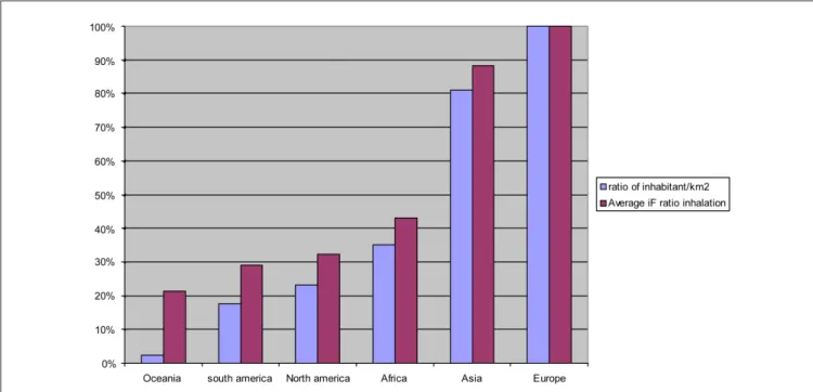
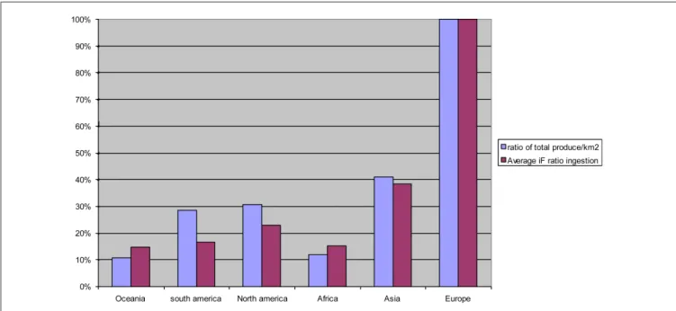
Figs. 2 and 3 show important differences in population
den-sity and food production per km2 of more than one order of magnitude. These variations in exposure parameters are likely to be reflected in significant variations between conti-nent-specific intake fractions.
2 Results and Discussion
2.1 Comparison of intake fractions (iF)
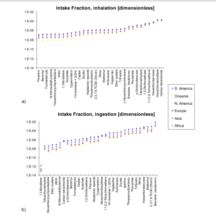
A set of representative organic, non-dissociating chemicals was used for this comparison, covering plausible differences in partitioning behavior, dominant human exposure pathways, overall environmental persistence, and long-range transport characteristics. Chemical properties were assumed to reflect variations under average conditions for a broad range of chemi-cals (Margni 2003). This dataset was also used within the OMNIITOX project (Molander et al. 2004). The model was run for a constant emission at the rate of 1 kg/hour in air in different continents, leading to calculation of the Intake Frac-tion, that is independent of the emission rate. First, the intake fraction for the entire set of substances is presented. Then, detailed results are illustrated and discussed for four specific substances selected on the basis of their widely different chemi-cal properties covering the combinations of high and low octanol-water partitioning coefficient, KOW, and high and low persistence in air (physical-chemical properties of the repre-sentative chemicals are given in the Supporting Information, online only, see DOI: http://dx.doi.org/10.1065/lca2006. 05.XXX). The cumulative risk is finally calculated for each chemical as the intake fraction is multiplied by the dose-response slope, which is assumed equal for all continents.
Fig. 4 shows the variation in intake fraction between
conti-nents for an emission to air. It enables to discuss how far these differences are important compared to the variability between substances. Intake fractions vary significantly up to about 102 between continents depending on the consid-ered substance. This is, however, still limited compared to the typical variation of 106 between substances for inges-tion. Interestingly, Fig. 4a shows that the variation between continents is very small for high intake fraction by inhala-tion. This corresponds to highly persistent substance in air, thus a more or less uniform concentration increase world-wide whatever the location of emission.
The ranking of the continents is almost the same for every substance. The magnitude of variation between continents is related to population density and to differences in the in-tensity of exposed food production as shown by the follow-ing detailed analysis on the four selected substances.
Production in (kg/year) Africa Asia Europe N America Oceania S America World
Unexposed produce 3.21⋅10+11 1.13⋅10+12 3.64⋅10+11 3.00⋅10+11 5.60⋅10+10 5.41⋅10+11 2.71⋅10+12 Exposed produce 1.84⋅10+11 1.46⋅10+12 5.51⋅10+11 5.28⋅10+11 4.41⋅10+10 1.53⋅10+11 2.92E+12
Fresh water fish 2.39⋅10+09 2.38⋅10+10 8.83⋅10+08 5.81⋅10+08 1.88⋅10+07 5.48⋅10+08 2.83⋅10+10 Pigs 6.98⋅10+08 4.84⋅10+10 2.50⋅10+10 1.16⋅10+10 4.73⋅10+08 3.01⋅10+09 8.91⋅10+10
Beef 4.26⋅10+09 1.37⋅10+10 1.16⋅10+10 1.55⋅10+10 2.58⋅10+09 1.18⋅10+10 5.95⋅10+10 Broilers 3.10⋅10+09 2.31⋅10+10 1.17⋅10+10 2.03⋅10+10 7.67⋅10+08 9.69⋅10+09 6.87⋅10+10
Goat and Sheep meat 1.80⋅10+09 6.03⋅10+09 1.48⋅10+09 2.08⋅10+08 1.23⋅10+09 3.32⋅10+08 1.11⋅10+10 Eggs 1.98⋅10+09 3.32⋅10+10 9.35⋅10+09 7.59⋅10+09 2.02⋅10+08 2.87⋅10+09 5.52⋅10+10
Dairy products (Cow milk) 2.50⋅10+10 1.69⋅10+11 2.10⋅10+11 9.74⋅10+10 2.35⋅10+10 4.49⋅10+10 5.70⋅10+11 Sea fish 6.07⋅10+09 2.77⋅10+10 1.05⋅10+10 6.83⋅10+09 5.75⋅10+09 1.74⋅10+10 7.42⋅10+10
Table 2: Production data in kg/year (source: FAOstat database)
Fig. 2: Population density (inhabitants/km2) in the 6 continents
2.2 Detailed iF analysis for four substances
Because of a relatively small KOW, tetrachloroethylene (Fig. 5a) does not bio-accumulate significantly, which explains the small intake fraction for this substance in agreement with the observations by Bennett et al. (2002a). The exposure is dominated by inhalation because of a relatively high Hen-ry's Law constant. Moreover, its relatively fast degradation rate in air competes with the air advection rates for large continents, such as Africa, Asia and Europe, implying that the intake is dominated by the continent of emission and do
not exceeds a fraction of 1 per 100,000: 1kg emitted causes a population intake of up to 10 mg. For less densely popu-lated continents, such as Oceania and South America, expo-sure occurs mainly at the global level and is one order of magnitude smaller.
Similarly to tetrachloroethylene, carbon tetrachloride (Fig. 5b) shows a low KOW and does not bio-accumulate. However, its partition to air (high Henry's Law constant) and persist-ence in the same medium is significantly higher (more than 1 order of magnitude) than for tetrachloroethylene. This leads
Fig. 4: Intake fraction variability for a dataset of 31 chemicals released to the air compartment of 6 different continental models (South America, Oceania,
to a higher intake fraction by inhalation that is rather uni-form worldwide. The continent-specific impacts are there-fore proportional to the population and higher for Asia, which accounts for half of the world population.
On the other hand, the next two substances, dioxine and
hexachlorobenzene have relatively low Henry Law constants
and high KOW, which means that pollutants tend to leave the air compartment and bioconcentrate in the food chain (Figs. 5c,d). The differences in air degradation explain that dioxin (relatively short half life in air) mainly affects the continent where it is emitted. Its high bioconcentration fac-tor in vegetable, milk and meat leads to very high intake fractions by ingestion of up to 1 per thousand, especially in Europe that shows the highest fraction of cultivated land, cou-pled with high agriculture production intensity (see Fig. 3). These values are in the same order of magnitude as experi-mentally based intake fraction for dioxin of 0.003 for Eu-rope (Margni et al. 2004) and 0.002 for USA (Bennett et al. 2002a). Hexachlorobenzene has a more uniform impact worlwide than dioxin because of its extremely high persist-ence in all environmental compartments.
2.3 Extrapolation for different continents
As shown by MacLeod et al. (2004), the intake fraction mostly varies according to different substance specific lin-ear regressions, as a function of the population density for inhalation and as a function of the food production rates for ingestion. However, in the context of continent-specific variation, it would be highly valuable to establish a more general relationship enabling extrapolating the intake
frac-tion of a wide range of substances, starting from the modeled intake fraction of a base continent – Europe in the case of Impact 2002. Figs. 4 and 5 suggest that the variability of the intake fraction between continents decreases as a function of the residence time in air, ultimately leading to a constant worldwide concentration and intake fraction. In other words, the higher the fraction advected from the specific continent to the world, the lower the variation between continents. Fol-lowing an analysis of the mass balance equations, we have therefore plotted the ratio of continental to European intake fractions by inhalation as a function of the fraction of the substance advected out of Europe (Fig. 6a). For local pollut-ant with little advection out of Europe, the iFic / iFiEurope ratio is
close to the ratio of the population densities ( ). This ratio increases linearly with the advected fraction up to one for very persistent substances.
The Intake fraction for a substance i emitted to air in a con-tinent c can therefore be approximated by the following re-lationship:
(2)
Where the ratio of population densities and the slope are given in Table 3.
Interestingly, for all continents but for Asia, the slope
inhalation
β
is close to 0.58, the R2 higher than 0.94 and the 95% confidence interval on individual prediction lower thanFig. 5: Intake fraction for an emission to air of tetrachloroethylene a), carbon tetrachloride b), 2,3,7,8-TCDD Dioxin c) and hexachlorobenzene d) detailed
15%. The higher variation with Asia (R2=0.84) is linked to the fact that Asia represents in itself 62% of the world popu-lation. For very persistent substances, a significant part of the advection out of Asia is nevertheless taken in later by
the Asian population itself. This feedback effect has been discussed in detail by Margni et al. (2004) and explains why the advected fraction can be higher than one for very per-sistent pollutants.
Fig. 6: Ratio of continental to European intake fractions (iFic / iFiEurope) for an emission to air as a function of the fraction advected out of Europe ( ), where the advection rate out of Europe is 0.00080 1/h and is the overall rate constant in air for substance i released in Europe. a) inhalation route b) ingestion route
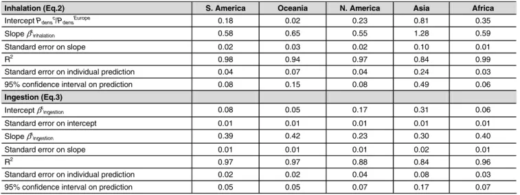
Table 3: Parameters and statistical data related to the extrapolation curves in Eqs. 2 and 3
Inhalation (Eq.2) S. America Oceania N. America Asia Africa
Intercept Pdensc/PdensEurope 0.18 0.02 0.23 0.81 0.35
Slope βcinhalation 0.58 0.65 0.55 1.28 0.59
Standard error on slope 0.02 0.03 0.02 0.10 0.01
R2 0.98 0.94 0.97 0.84 0.99
Standard error on individual prediction 0.04 0.07 0.04 0.24 0.03 95% confidence interval on prediction 0.08 0.15 0.08 0.49 0.06
Ingestion (Eq.3)
Intercept βc
ingestion 0.08 0.05 0.17 0.31 0.06
Standard error on intercept 0.01 0.01 0.01 0.01 0.01
Slope βc
ingestion 0.39 0.42 0.23 0.30 0.40
Standard error on slope 0.01 0.01 0.01 0.02 0.01
R2 0.97 0.97 0.88 0.84 0.96
Standard error on individual prediction 0.02 0.02 0.04 0.08 0.03 95% confidence interval on prediction 0.05 0.05 0.07 0.17 0.07
Similar figures and equations can be established for the in-gestion pathway (Fig. 6b). As shown in the Supporting
In-formation (online only, see DOI: http://dx.doi.org/10.1065/
lca2006.05.xxx), the intercept is related to the amount of food produced per unit area in each continent. It is espe-cially the exposed vegetation that dominates the intake in most cases, except for a few substances, for which milk and meat are significant. The relationship is, however, not as direct as with the population densities for inhalation, due to the variety of intake pathways and to the variation in veg-etation volume across continents. The corresponding ap-proximation for ingestion is therefore given by:
(3) where the intercept value αingestion and the slope βingestion are
given in Table 3 for each continent.
The proposed correlation explains more than 84% of the variability and even more than 96% for Oceania, Africa and South America.
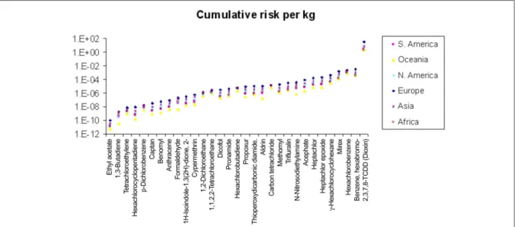
2.4 Overall cumulative risks
Once intake fractions are combined with effect factors as proposed by Crettaz and colleagues (Crettaz et al. 2002, Pennington et al. 2002), cumulative risks vary significantly of about 102 between continents depending on the consid-ered substance (Fig. 7). This is, however, relatively low com-pared to the variation of 1012 between substances.
3 Conclusion
This project showed the feasibility to readily determine ge-neric characterization factors for different geographical world regions, using publicly available data to parameterize
multimedia and multipathways exposure. Results show that despite important variations in characterization factors rela-tive to which continent the pollutant is emitted:
• this remains restricted to two orders of magnitude com-pared the variations of the entire set that achieves up to twelve orders of magnitude, and
• the ranking tends to remain constant supporting the choice to use of generic characterization factors, as sug-gested in common life cycle impact assessment methods, for LCA studies.
The main parameters affecting continent-specific variations are the population density for the inhalation route and the total agricultural production for the ingestion route of ex-posure confirming the findings of MacLeod et al. (2004). The study of four substances also showed that population density and agriculture cultivated areas may affect the mag-nitude and location of the impact, which may happen out-side the continent in which the substance is emitted. The more persistent the substance is, the higher the impact out-side its continent of emission and the less variation is ob-served between continents.
Generic characterization factors are not sufficiently precise to determine absolute values or to compare impacts from two scenarios whose major emissions takes place in different con-tinents. In this case, the continent specific characterization fac-tors should be considered. The main parameters affecting con-tinent-specific variations are the population density for the inhalation route and the total agricultural production for the ingestion route of exposure. For this purpose we proposed a simplified method enabling extrapolating continent specific intake fractions of a wide range of substances, starting from the modeled intake fraction of a base continent as a function of the fraction of the chemical advected out of the region. Eqs. 2 and 3 enable to extrapolate the intake fraction for any continent, based on the European intake fraction, with more than 84% of the variability explained. The 95% confidence
interval of 5% to 50% are low compared to the overall vari-ation in intake fraction of 6 to 10 orders of magnitude and the 12 orders of magnitude in cumulative risk. This simpli-fied method could be readily adapted to extrapolate conti-nent-specific iF for any other model. As these results and correlations refer to an air emission scenario, they need to be further extended to consider other media of release, re-sulting in potentially different spatial variabilities and cor-relations. It would also be highly interesting to test the pro-posed regression at national or regional, taking profit of the GLOBACK database (Wegener Sleeswijk 2005).
As impact in the world box can even be dominant for some chemical, further research should focus on linking the differ-ent contindiffer-ental boxes to obtain a global spatial model compa-rable to the European spatial model (Pennington et al. 2005) or to extend the world model proposed by Toose and col-leagues (Toose et al. 2004) by adding exposure to the fate modeling. The level of spatial resolution has to be carefully selected: The aim is to capture significant differences, but at the same time to avoid unnecessarily requirement efforts for data gathering and calculation capabilities. Moreover, some major climatic phenomenon must be included in the modeling, such as considering an upper air level to include high alti-tude inter continental substance transport by jet stream.
References
Bennett DH, Margni M, McKone TE, Jolliet O (2002a): Intake Fraction for Multimedia Pollutants: A Tool for Life Cycle Analysis and Comparative Risk Assessment. Risk Analysis 22 (5) 903–916
Bennett DH, McKone TE, Evans JS, Nazaroff WW, Margni MD, Jolliet O, Smith KR (2002b): Defining Intake Fraction. Environ Sci Technol 36 (9) 207A–211A
Bey I, Jacob DJ, Yantosca RM, Logan JA, Field B, Fiore AM, Li Q, Liu H, Mickley LJ, Schultz M (2001): Global modeling of tropospheric chemis-try with assimilated meteorology: Model description and evaluation. J Geophys Res 106, 23073–23096
Brandes LJ, den Hollander H, van de Meent D (1996): SimpleBox 2.0: A Nested Multimedia Fate Model for Evaluating the Environmental Fate of Chemicals, 719101029. RIVM, The Netherlands
CIA (2004): The World Factbook. <http://www.cia.gov/cia/publications/ factbook/>
Cowan CE, Mackay D, Feijtel TCJ, van de Meent D, Di Guardo A, Davies J, Mackay N (eds) (1994): The Multi-Media Fate Model: A Vital Tool for Predicting the Fate of Chemicals. SETAC. SETAC Press, Denver, CO and Leuven, Belgium
Crettaz P, Pennington D, Rhomberg L, Brand B, Jolliet O (2002): Assessing Human Health Response in Life Cycle Assessment Using ED10s and DALYs: Part 1 – Cancer Effects. Risk Analysis 22 (5) 931–946 FAO (2004): FAO Statistical Databases. <http://www.fao.org>
Global Runoff Data Centre (2004): World Runoff Data. <www.grdc.sr.unh.edu/> Goedkoop M, Effting S, Collignon M (2000): The Eco-indicator 99: A dam-age oriented method for Life Cycle Impact Assessment, PRé Consultants B.V., Amersfoort, The Netherlands
Goedkoop M, Müller-Wenk R, Hofstetter P, Spriensma R (1999): The Eco-Indicator 99 Explained. Int J LCA 3 (6)
Guinee J, Heijungs R, van Oers L, Sleeswijk A, van de meent D, Vermeire T, Rikken M (1996): Inclusion of Fate in LCA Characterization of Toxic Releases Applying USES 1.0. Int J LCA 1, 118–133
Hertwich E, Matales SF, Pease WS, McKones TE (2001): Human Toxicity Potentials for Life-Cycle Assessment and Toxics Release Inventory Risk Screening. Environmental Toxicology and Chemistry 20 (4) 928–939 Huijbregts MAJ, Lundi S, McKone TEl, van de Meent D (2003):
Geographi-cal scenario uncertainty in generic fate and exposure factors of toxic pol-lutants for life-cycle impact assessment. Chemosphere 51 (6) 501–508 Huijbregts MAJ, Thissen U, Guinee JB, Jager T, Kalf D, van de Meent D,
Ragas AMJ, Wegener Sleeswijk A, Reijnders L (2000): Priority assess-ment of toxic substances in life cycle assessassess-ment. Part I: Calculation of Toxicity potentials for 181 substances with the nested multi-media fate, exposure and effects model USES-LCA. Chemosphere 41, 541–573
Itsubo N, Inaba A (2003): A new LCIA method: LIME has been completed. Int J LCA 8 (5) 305
Jolliet O (1996): Impact assessment of human and eco-toxicity in Life Cycle Assessment. In: Udo de Haes HA (ed), Towards a Methodology for Life Cycle Impact Assessment SETAC Europe Press, Brussels, Belgium Jolliet O, Margni M, Humbert S, Payet J, Rebitzer G, Rosenbaum R (2003):
IMPACT 2002+: A New Life Cycle Impact Assessment Methodology. Int J LCA 8(6) 324–330
Jolliet O, Müller-Wenk R, Bare JC, Brent A, Goedkoop M, Heijungs R, Itsubo N, Peña C, Pennington D, Potting J, Rebitzer G, Stewart M, Udo de Haes H, Weidema B (2004): The LCIA Midpoint-damage Frame-work of the UNEP/SETAC Life Cycle Initiative. Int J LCA 9 (6) 394–404 Klepper O, den Hollander HA (1999): A comparison of spatially explicit and box models for the fate of chemicals in water, air and soil in Europe. Ecological Modelling 116, 183–202
MacLeod M, Bennett D, Perem M, Maddalena R, McKone T, Mackay D (2004): Dependence of Intake Fraction on Release Location in a Multi-media Framework: A Case Study of Four Contaminants in North America. Journal of Industrial Ecology 8 (3) 89–102
MacLeod M, Woodfine DG, Mackay D, McKone T, Bennett DMaddalena R (2001): BETR North America: A regionally segmented multimedia contaminant fate model for North America. Environmental Science and Pollution Research 8 (3) 156–163
Margni M (2003): Source to Intake Modeling in Life Cycle Impact Assess-ment. Section Science et Ingénierie de l'EnvironneAssess-ment. Lausanne, Swiss Federal Institute of Technology (EPFL), p 138
Margni M, Pennington DW, Amman C, Jolliet O (2004): Evaluating multi-media/multipathway model intake fraction estimates using POP emis-sion and monitoring data. Environmental Pollution 128, 263–277 McKone TE (1993): CalTOX, A Multimedia Total-Exposure Model for
Hazardous-Wastes Sites, UCRL-CR-111456PTI. Lawrence Livermore National Laboratory, Livermore, CA
McKone TE, Bodnar A, Hertwich EG (2001): Development and Evalua-tion of State-Specific Landscape Data Sets Regional Multimedia Mod-els. Lawrence Berkeley National Laboratory Report No. LBNL-43722, July, 2001
Molander S, Lidholm P, Schowanek D, Recasens M, Fullana i Palmer P, Christensen F, Guinée JB, Hauschild M, Jolliet O, Carlson R, Pennington DW, Bachmann TM (2004): OMNIITOX – Operational Life-Cycle Im-pact Assessment Models and Information Tools for Practitioners. Int J LCA 9 (5) 282–288, <http://www.omniitox.net>
Pennington D, Crettaz P, Tauxe A, Rhomberg L, Brand B, Jolliet O (2002): Assessing Human Health Response in Life Cycle Assessment Using ED10s and DALIs: Part 2 – Noncancer Effects. Risk Analysis 22 (5) 947–963 Pennington DW, Margni M, Amman C, Jolliet O (2005): Multimedia fate
and human intake modeling: Spatial versus nonspatial Insights for chemical emissions in Western Europe. Environ Sci and Technol 39 (4) 1119–1128
Prevedouros K, MacLeod M, Jones KC, Sweetman AJ (2004): Modelling the fate of persistent organic pollutants in Europe: Parameterisation of a grided distribution model. Environ Pollut 128, 251–261
Stewart MJolliet O (2004): User needs analysis and development of priori-ties for life cycle impact assessment. Int J LCA 9 (3) 153–160 Toose L, Woodfine DG, MacLeod M, Mackay D, Gouin J (2004):
BETR_World: a geograpnically explicit model of chemical fate: applica-tion to transport of alpha-HCH to the Arctic. Environmental Polluapplica-tion 128, 223–240
Udo de Haes H, Jolliet O, Finnveden G, Goedkoop M, Hauschild M, Hertwich E, Hofstetter P, Klöpffer W, Krewitt W, Lindeijer E, Mueller-Wenk R, Olson S, Pennington D, Potting J, Steen B (2002): Towards best available practice in Life Cycle Impact Assessment. SETAC Press, Pensacola, Florida, US
Wegener Sleeswijk A (2005): GLOBACK (Version 1.0). Environmental pa-rameters of the GLOBOX model. Part 1: Fate and Exposure. Part 2: Boundaries and water flows. Institute of Environmental Sciences (CML), Leiden University, Leiden, The Netherlands. Available at: <http:// www.leidenuniv.nl/interfac/cml/ssp/index.html>
Received: February 17th, 2006 Accepted: February 23rd, 2006
OnlineFirst: February 24th, 2006
Appendix: Supporting information
The appendix can be found in the online edition of this paper. You can access the online edition via the website <DOI: http://dx.doi.org/ 10.1065/lca2006.05.012>
Supporting Information (online only)
1 Physical-chemical Properties of the Set of
Representative Organic, Non-dissociating Chemicals
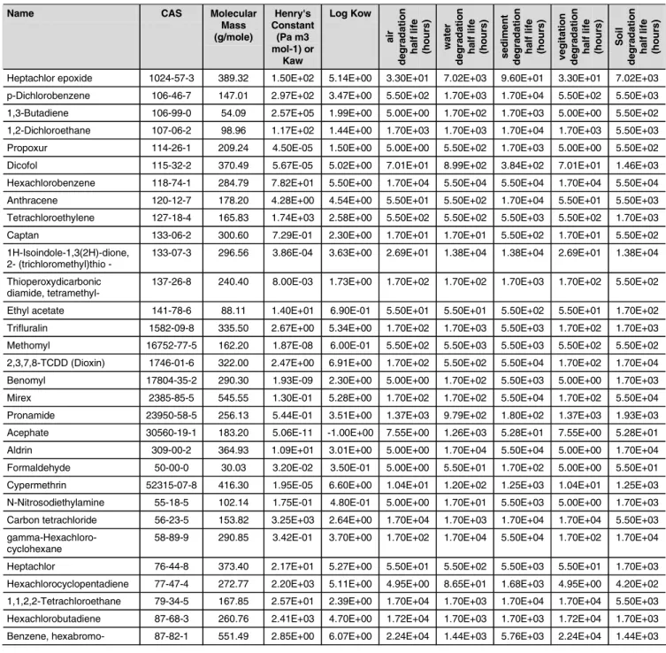
Chemicals in Table S1 were selected from approximately 500 non-dissociating organic chemicals using data adopted analo-gous to US EPA's draft WMPT tool data selection hierarchy (USEPA 1998). Data are from, in order of typically preference adopted, Mackay et al. data compilation handbooks (Mackay et al. 1995), Howard et al. data compilation handbooks (Howard 1991, Howard et al. 1991), Physprop
experimen-tal data (Syracuse Research Corporation), Epiwin experi-mental data (Howard et al. 2002), Physprop estimated data (Syracuse Research Corporation), Epiwin estimated data (Howard et al. 2002). Data gaps were additionally filled using the CalTox model (McKone et al. 2001) and the USES-LCA model (Howard et al. 2002) databases.
Table S1: Physical-chemical properties of the set of 31 representative organic, non-dissociating chemicals
Name CAS Molecular
Mass (g/mole) Henry's Constant (Pa m3 mol-1) or Kaw Log Kow air d e gr a d a ti o n ha lf l if e (h o u rs ) wate r d e gr a d a ti o n ha lf l if e (h o u rs ) sed im en t d e gr a d a ti o n ha lf l if e (h o u rs ) veg ita ti o n d e gr a d a ti o n ha lf l if e (h o u rs ) Soi l d e gr a d a ti o n ha lf l if e (h o u rs )
Heptachlor epoxide 1024-57-3 389.32 1.50E+02 5.14E+00 3.30E+01 7.02E+03 9.60E+01 3.30E+01 7.02E+03 p-Dichlorobenzene 106-46-7 147.01 2.97E+02 3.47E+00 5.50E+02 1.70E+03 1.70E+04 5.50E+02 5.50E+03 1,3-Butadiene 106-99-0 54.09 2.57E+05 1.99E+00 5.00E+00 1.70E+02 1.70E+03 5.00E+00 5.50E+02 1,2-Dichloroethane 107-06-2 98.96 1.17E+02 1.44E+00 1.70E+03 1.70E+03 1.70E+04 1.70E+03 5.50E+03 Propoxur 114-26-1 209.24 4.50E-05 1.50E+00 5.00E+00 5.50E+02 1.70E+03 5.00E+00 5.50E+02 Dicofol 115-32-2 370.49 5.67E-05 5.02E+00 7.01E+01 8.99E+02 3.84E+02 7.01E+01 1.46E+03 Hexachlorobenzene 118-74-1 284.79 7.82E+01 5.50E+00 1.70E+04 5.50E+04 5.50E+04 1.70E+04 5.50E+04 Anthracene 120-12-7 178.20 4.28E+00 4.54E+00 5.50E+01 5.50E+02 1.70E+04 5.50E+01 5.50E+03 Tetrachloroethylene 127-18-4 165.83 1.74E+03 2.58E+00 5.50E+02 5.50E+02 5.50E+03 5.50E+02 1.70E+03 Captan 133-06-2 300.60 7.29E-01 2.30E+00 1.70E+01 1.70E+01 5.50E+02 1.70E+01 5.50E+02 1H-Isoindole-1,3(2H)-dione,
2- (trichloromethyl)thio -
133-07-3 296.56 3.86E-04 3.63E+00 2.69E+01 1.38E+04 1.38E+04 2.69E+01 1.38E+04 Thioperoxydicarbonic
diamide, tetramethyl-
137-26-8 240.40 8.00E-03 1.73E+00 1.70E+02 1.70E+02 1.70E+03 1.70E+02 5.50E+02
Ethyl acetate 141-78-6 88.11 1.40E+01 6.90E-01 5.50E+01 5.50E+01 5.50E+02 5.50E+01 1.70E+02 Trifluralin 1582-09-8 335.50 2.67E+00 5.34E+00 1.70E+02 1.70E+03 5.50E+03 1.70E+02 1.70E+03 Methomyl 16752-77-5 162.20 1.87E-08 6.00E-01 5.50E+02 5.50E+03 5.50E+03 5.50E+02 5.50E+02 2,3,7,8-TCDD (Dioxin) 1746-01-6 322.00 2.47E+00 6.91E+00 1.70E+02 5.50E+02 5.50E+04 1.70E+02 1.70E+04 Benomyl 17804-35-2 290.30 1.93E-09 2.30E+00 5.00E+00 1.70E+02 5.50E+03 5.00E+00 1.70E+03 Mirex 2385-85-5 545.55 1.30E-01 5.28E+00 1.70E+02 1.70E+02 5.50E+04 1.70E+02 5.50E+04 Pronamide 23950-58-5 256.13 5.44E-01 3.51E+00 1.37E+03 9.79E+02 1.80E+02 1.37E+03 1.93E+03 Acephate 30560-19-1 183.20 5.06E-11 -1.00E+00 7.55E+00 1.26E+03 5.28E+01 7.55E+00 5.28E+01 Aldrin 309-00-2 364.93 1.09E+01 3.01E+00 5.00E+00 1.70E+04 5.50E+04 5.00E+00 1.70E+04 Formaldehyde 50-00-0 30.03 3.20E-02 3.50E-01 5.00E+00 5.50E+01 1.70E+02 5.00E+00 5.50E+01 Cypermethrin 52315-07-8 416.30 1.95E-05 6.60E+00 1.04E+01 1.20E+02 1.25E+03 1.04E+01 1.25E+03 N-Nitrosodiethylamine 55-18-5 102.14 1.75E-01 4.80E-01 5.00E+00 1.70E+01 5.50E+03 5.00E+00 1.70E+03 Carbon tetrachloride 56-23-5 153.82 3.25E+03 2.64E+00 1.70E+04 1.70E+03 1.70E+04 1.70E+04 5.50E+03
gamma-Hexachloro-cyclohexane
58-89-9 290.85 3.42E-01 3.70E+00 1.70E+02 1.70E+04 5.50E+04 1.70E+02 1.70E+04 Heptachlor 76-44-8 373.40 2.17E+01 5.27E+00 5.50E+01 5.50E+02 5.50E+03 5.50E+01 1.70E+03 Hexachlorocyclopentadiene 77-47-4 272.77 2.20E+03 5.11E+00 4.95E+00 8.65E+01 1.68E+03 4.95E+00 4.20E+02 1,1,2,2-Tetrachloroethane 79-34-5 167.85 2.57E+01 2.39E+00 1.70E+04 1.70E+03 1.70E+04 1.70E+04 5.50E+03 Hexachlorobutadiene 87-68-3 260.76 2.41E+03 4.70E+00 1.72E+04 1.70E+03 1.70E+03 1.72E+04 1.70E+03 Benzene, hexabromo- 87-82-1 551.49 2.85E+00 6.07E+00 2.24E+04 1.44E+03 5.76E+03 2.24E+04 1.44E+03
2 Main Exposure Pathways
It is mostly the exposed vegetal products that dominate the intake in most cases, except for a few substances, for which fish, milk and meat are significant (Fig. S1).
Fig. S1: Distribution of the intake by ingestion for the different intake pathways. Chemical are ordered by increasing ingestion intake fraction
3 Average Intake Fractions for Different Continents
Taking the European continent as a reference, Fig. S2 plots the average reduction in intake fraction for other continents. For the inhalation route of exposure, the reduction in iF amounts up to a factor 5 and is indeed strongly correlated
to the relative reduction in population density (Fig. S2a: R2=0.99). For ingestion, reduction in iF of up to a factor 10 on average is strongly correlated to the total agriculture pro-duction per km2 (Fig. S2b: R2=0.97).
References
Howard PH, Meylan W, Boethling R (2002): 'EPWIN Suite'. <http://www.syrres.com/esc/>
Howard PH (1991): Handbook of Environmental Fate and Ex-posure Data. Chelsea, MI, Lewis Publishers
Howard PH, Boethling RS, Jarvis WF, Meylan WM, Michalenko EM (1991): Handbook of Environmental Degradation Rates. Michigan, Lewis Publishers
Mackay D, Shiu WY, Ma KC (1995): Illustrated Handbook of Physical-Chemical Properties and Environmental Fate for Or-ganic Chemicals. Boca Raton, Lewis Publishers
Fig. S2b: Average continental intake fraction by ingestion compared to the total agriculture production per km2. All data are normalized to Europe (100%)
McKone T, Bennett D, Maddalana R (2001): CalTOX 4.0 Tecnical Support Document, Vol. 1. Berkeley, CA, Lawrence Berkeley National Laboratory
Syracuse Research Corporation. (2002): 'PhysProp chemical prop-erty database'. Merrill Lane, Syracuse, New York 132-4080. <http://www.syrres.com/esc/>
USEPA (1998): Notice of availability of draft RCRA waste mini-mization PBT chemical list