I
mpact of a stochastic sequential initiation of fractures
on the spatial correlations and connectivity
of discrete fracture networks
François Bonneau1, Guillaume Caumon1, and Philippe Renard2
1GeoRessources, UMR-7359 Université de Lorraine-ENSG/CNRS/CREGU, Nancy, France, 2Centre d’hydrogéologie et de
géothermie, Université de Neuchatel, Neuchatel, Switzerland
Abstract
Stochastic discrete fracture networks (DFNs) are classically simulated using stochastic point processes which neglect mechanical interactions between fractures and yield a low spatial correlation in a network. We propose a sequential parent-daughter Poisson point process that organizes fracture objects according to mechanical interactions while honoring statistical characterization data. The hierarchical organization of the resulting DFNs has been investigated in 3-D by computing their correlation dimension. Sensitivity analysis on the input simulation parameters shows that various degrees of spatial correlation emerge from this process. A large number of realizations have been performed in order to statistically validate the method. The connectivity of these correlated fracture networks has been investigated at several scales and compared to those described in the literature. Our study quantitatively confirms that spatial correlations can affect the percolation threshold and the connectivity at a particular scale.1. Introduction
Fracture networks in rock masses significantly affect hydrodynamic and geomechanical processes. Due to incomplete observations and measurements at all relevant scales, numerical modeling is widely used to describe the geometry and understand the behavior of fractured rocks. However, efficiently honoring both statistical descriptions of the fractured medium and all the physical principles driving fracture genesis remains a challenge. This paper reports on investigations to integrate physical and geological principles in stochastic discrete fracture network (DFN) simulations and assessing the impact of this integration on emerging DFN properties such as network connectivity and fractal dimension.
Spatial characteristics of subsurface fracture networks are the result of complex processes. These processes have been described by linear elastic fracture mechanics and studies about the initiation, growth, interaction, and termination of fractures [Olson, 1993; Renshaw and Pollard, 1994; Tuckwell et al., 2003; Jing, 2003; Welch et al., 2009]. Fractures initiate at rock flaws [Pollard and Aydin, 1988; Cosgrove and Engelder, 2004]. Heterogeneities such as fossils, grains, cavities, microcracks, and other objects having elastic properties dif-ferent from those of the surrounding rock modify the stress field in such a way that the magnitude of local stresses may exceed the strength of the rock, thereby initiating a fracture. Fractures create local hetero-geneities in both the stress field and the bulk properties of the rock. Pollard and Aydin [1988] describe the decrease of mechanical stress along cracks (in the shadow zone) and its increase at fracture tips (in the stress concentration zone). Fractures then grow as long as the effective stress locally exceeds the strength of the rock [Griffith, 1921, 1924]. Numerical modeling of this process requires to evaluate the stress state everywhere and at all times in the simulation domain. It is generally based on boundary conditions and uses finite ele-ment, boundary eleele-ment, or discrete element methods which are computationally intensive for large scale 3-D problems and are often subject to gridding and discretization problems. Therefore, stochastic approaches are often applied for efficiently simulating very large fracture networks (for reviews, see, e.g., Jing [2003], Chilès [2005], Dershowitz et al. [2004], Dowd et al. [2007, and see also De Dreuzy et al. [2013] for a benchmark). Stochastic approaches do not solve the mechanical problem but aim at defining a mathematical proxy that reproduces the final geometry of natural fracture networks. Those methods rely on the statistical inference and characterization of the fracture network from field and analog observations.
Classical stochastic discrete fracture network simulations consider fractures as simple 2-D objects (rectangles or ellipses) in 3-D space. The position of rock flaws stimulated by the stress field is usually generated either
Key Points:
• The proposed method accounts for fracture interactions during 3-D discrete fracture implantation • Mechanical interactions affect the
emerging fractal dimension of the network
• Spatial correlations induced by this method may change the network’s percolation threshold
Correspondence to:
F. Bonneau,
by a homogeneous or heterogeneous Poisson point process [Stoyan and Stoyan, 1994; Lantuéjoul, 2002]. The dimension and orientation of the fracture are simulated for each object independently by sampling from prior probability distribution functions with a Monte Carlo process. This approach generally simulates frac-ture set by set following their chronology in relation to tectonic events [e.g., Mace et al., 2005; Yamaji and
Sato, 2011; Lamarche et al., 2012]. However, the geometry and the position of each fracture in each set is
ran-domly and independently selected. Even if the statistics describing each set are honored, the flow behavior and emerging fracture network features such as connectivity and spatial correlations may be biased. This is attested, for instance, by Odling and Webman [1991] who highlight in two dimensions the differences of global permeability between natural and simulated fracture networks sharing the same length and orientation statistics.
This problem can be addressed by several improvements to Poisson-based DFN simulation methods. An avenue is to refine the statistical models used in the DFN simulation, see, for instance, Chilès [1988] and Xu and Dowd [2010]. Another is to incorporate the effects of mechanical interactions which control fracture initiation, growth, and arrest. This has been done by reproducing the effects of these interactions on the fracture geom-etry [Josnin et al., 2002], and mimicking the fracture growth using planar fractures [Cladouhos and Marrett, 1996; Swaby and Rawnsley, 1996; Davy et al., 2013] or nonplanar fractures [Cacas et al., 2001; Srivastava et al., 2005; Bonneau et al., 2013]. Among these methods, Cladouhos and Marrett [1996] relate a simplified two-dimensional linkage model to the emergence of power law distributions. Similarly, Davy et al. [2013] establish theoretical and numerical links between fracture seeding and development processes and emerg-ing fracture statistics in simulated DFNs (density and power law length distribution). In this paper, we use similar ideas to evaluate numerically the link between pseudomechanical DFN simulation and emerging char-acteristics such as the connectivity and fractal dimension. For this, we propose a simulation method which emulates the stress perturbation effects around fractures during their seeding. This numerical method aims at both reproducing the statistics describing natural fracture networks and the geometrical hierarchy between fractures. The main idea is to use a sequential parent-daughter Poisson point process that favors the initia-tion of small fractures at the tips of larger fractures (secinitia-tion 2). A large number of realizainitia-tions is performed on synthetic data to validate the method in a statistical sense. We discuss and quantify the impact of this sequential fracture seeding on the DFNs organization in terms of spatial correlation (section 3), connectivity, and percolation (section 4).
2. Sequential Stochastic Discrete Fracture Network Simulation
Several pseudogenetic approaches have been proposed to simulate fracture geometry by propagating frac-tures from an initial state using simple mechanical concepts on growth and arrest [Josnin et al., 2002; Srivastava et al., 2005; Bonneau et al., 2013; Davy et al., 2013]. Instead, this work focuses on the fracture nucleation to capture hierarchical organization of natural fracture networks.
We are making the assumption that fracture radial growth and coalescence are correctly described by the length distribution law. Objects are progressively implanted in their final state, and so we neglect the fracture growth, interaction, and coalescence that lead to the final fracture geometry. Large fractures are simulated first because they have grown far from discontinuities that may interact and stop their growth. We use an approximate local stress perturbation model (Figure 1 and section 2.1) to later organize small fractures around these major objects with a probabilistic acceptance of fracture seeds (section 2.2).
2.1. Simplified Fracture Object
Produced DFNs are made of planar objects characterized by their position, extension, and orientation. These objects may represent either a single or several coalesced discontinuities. Each fracture is associated to a simplified stress perturbation model that represents the shadow and the stress concentration zones. Several authors have integrated such simplified geomechanical models in stochastic DFN simulations [Cladouhos and
Marrett, 1996; Srivastava et al., 2005; Bonneau et al., 2013]. Most of them used a spherical isotropic model.
In this work, we use a simple model constituted by two ellipsoids in order to take into account the anisotropy often observed in stress concentration around fracture tips (Figure 1) [Lyakhovsky, 2001].
These ellipsoids separate volumes where the probability to observe a crack is increased (respectively, decreased) because of the stress concentration (respectively, relaxed). The geometry of each ellipsoid is defined by factors weighting the fracture size: (𝛼s, 𝛽s) for shadow zone and (𝛼p, 𝛽p) for stress concentra-tion zone. This model, inspired by the shape of symmetric stress perturbaconcentra-tion around tensile fractures,
Figure 1. Simplified 3-D stress model around a fracture. Two ellipsoids individualize the stress concentration zone
(in blue) and the shadow zone (in red). Note that the intersection between the blue and the red ellipsoids is a part of the shadow zone. The extent of each zone is deduced from fracture dimensions by applying scaling factors (𝛼s, 𝛼p, 𝛽s, and 𝛽p). In this figure, we set 𝛼s = 1, 𝛽s = 1, 𝛼p = 2, and 𝛽p = 0.5.
aims at approximating the first-order stress perturbation of all types of fractures. This may be locally inconsis-tent (e.g., if fractures are parallel to the main compressive stress direction). However, far-field stress is generally not known during DFN simulation, so this model is expected to emulate geomechanical effects on average (section 5).
The next section describes a stochastic simulation process that uses these ellipsoids to drive the seeding of fractures.
2.2. Sequential Parent-Daughter Poisson Point Process
Our global sequential seeding process is described in Appendix A and Figure 2. It uses a heterogeneous Poisson point process that generates N potential fracture seeds according to a prior fracture density map (d(x,y,z)) that may be obtained by strain analysis [Cacas et al., 2001; Mace et al., 2005], seismic methods
Figure 2. One seeding sequence follows several steps. (a) Fractures simulated previously and their associated influence
zones. They will drive the activation of new fractures during further steps. The classical Poisson point process generates possible fracture center locations ((b) following a uniform density in this example). (c) Activated fractures are then selected following equation (1).
[Sayers, 2009; Serrano et al., 2014; Rodriguez-Herrera et al., 2015], or other ancillary observations. Then the nucleation of fractures uses a probabilistic acceptance/rejection test that takes into account the fractures pre-viously simulated. Simulation is then performed in a given number of sequences (s ∈ [1, N]). During the first seeding sequence, the probability (P(x,y,z)) to simulate a fracture at a position generated by the Poisson point process is uniform and equal toN
s
1
N = 1∕s.
Planar fractures are simulated by a Monte Carlo sampling of orientation and dimension distribution laws. Around each simulated fracture, a simplified geomechanical model (Figure 1) divides the volume of interest into several parts in which the prior probability (P(x,y,z)) to activate a fracture at a given seed (x, y, z) has to be locally adjusted considering the following.
1. The impact (g) and the number (Nacc(x, y, z)) of stress concentration zones overlapping the (x, y, z) location.
The probability to stimulate a rock flaw inside stress concentration zones is increased by a factor g≥ 1. 2. The impact (h) and the number (Nacc(x, y, z)) of shadow zones defined at the (x, y, z) location. The
condi-tional probability to stimulate a rock flaw inside the shadow zone is decreased by a factor h≥ 1.
h and g are input parameters standing for the impact of shadow and stress concentration zones. As a consequence, we define the adjusted probability Ps
(x,y,z)at each step of a process divided in s sequences as follows: Ps (x,y,z)= N s (1 + g × N acc(x, y, z) 1 + h × Nshad(x, y, z) ) ∕ (N ∑ i=1 1 + g × Nacc(x, y, z)i 1 + h × Nshad(x, y, z)i ) (1)
For each seeding sequence, the Poisson point process simulates N seeds that are scanned twice (algorithm in Appendix A). The first iteration evaluates the denominator of equation (1) by counting Nacc (weighted by g) and Nshad (weighted by h) for each seed. The second iteration uses the previous result that quan-tifies the fracturing state to compute and normalize P(x,y,z) according to the impact of already simulated fractures.
The proportion of stress concentration/relaxation zones (Figure 1) depends on both the fracture length and on the number of simulated fractures. In other words, the proportion of these zones depends on the fracture density. In the early stage, only a few fractures have been activated and the fracturing process is not strongly impacted by previous fractures. In this case, every fracture center proposed by the Poisson point process has the same probability (P(x,y,z)= 1∕s) to be selected for simulation because Nacc(x, y, z) ≈ Nshad(x, y, z) ≈ 0. During the simulation, the number of fractures increases and consequently their impact on the simulation process increases as well. Finally, the method naturally reproduces the “poorly” and “well-developed” fracture networks [Wu and Pollard, 1995] as well as the transition regime between these two states [Davy et al., 2010]. “Poorly” and “well-developed” fracture networks have also been described in terms of “unsaturated” and “saturated” [Josnin et al., 2002] or “dilute” and “dense” fracture networks [Davy et al., 2010].
This approach organizes small fracture objects at the tips of longest ones. It neglects the interaction between fractures during their growth and the fractures that are nucleated during the fracture growth. As a result, our method may underestimate the number of fractures that initiate from older fractures, which may lead to an underestimation of the network connectivity. Strategies to incorporate the effects of interactions during fracture growth should therefore be considered in future research.
2.3. Impact on DFN Spatial Correlation
In this section, we analyze the DFN spatial correlations emerging from the above sequential seeding process. A quantitative characterization of spatial correlations is also possible using fractal theory. This aspect has been much studied in the literature for its ability to describe natural fracture systems [Mandelbrot, 1983; Velde et al., 1991; Ouillon et al., 1996; Bour and Davy, 1999; Bour et al., 2002; Darcel et al., 2003]. The measurement of the fractal dimension of fracture networks can be related to several definitions that quantify the singularities of the multifractal spectrum. Bonnet et al. [2001] present a review for characterizing and estimating the capacity dimension, the information dimension, and the correlation dimension that can be considered as the three first moments of the multifractal spectrum.
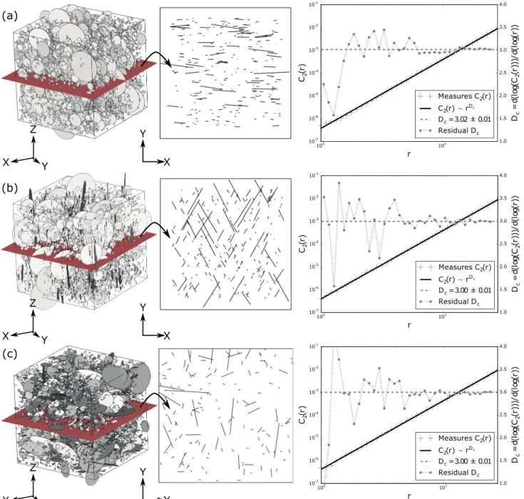
Figure 3. The 3-D and 2-D views of DFNs obtained with the Poisson point process for (a) a single fracture set DFN, (b) a two fracture set DFN, and (c) a DFN
where fractures are randomly oriented. The 2-D views show the traces of fractures on the red slice. Fractures are uniformly positioned in space. Graphs show for each kind of DFN the correlation function estimationC2(r)in black and the estimation of the DFN correlation dimensionDcin grey. As the fractal dimension is approximately 3, the experiments show that the classical Poisson point process generates uncorrelated DFNs.
In this work, we quantify the correlation dimension Dc of fracture network models using a pair correla-tion funccorrela-tion (C2(r)) computed from the fracture center repartition, similar to Davy et al. [1990] and Bour
et al. [2002]:
C2(r) =
2 × N(r) Nt× (Nt− 1)
≈ rDc (2)
where N(r) is the number of pairs of fracture centers whose separation distance is less than r. Ntis the total number of fracture centers in the considered volume of rock. Ouillon et al. [1996] and Bonnet et al. [2001] have shown that computing the correlation dimension using equation (2) provides more accurate spatial
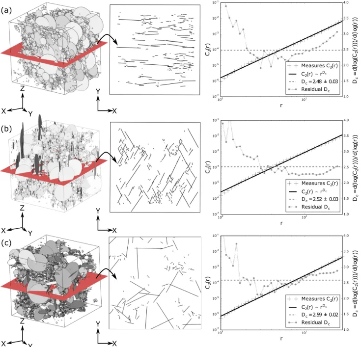
Figure 4. The 3-D and 2-D views of DFNs obtained with the sequential parent-daughter Poisson point process for (a) a single fracture set DFN, (b) a two fracture
set DFN, and (c) a DFN where fractures are randomly oriented. The 2-D views show the traces of fractures on the red slice. Fractures seem organized. The seeding process entails a spacing between fractures and attracts small fractures at larger fracture tips. Graphs show for each kind of DFN the correlation function estimationC2(r)in black and the estimation of the DFN correlation dimensionDcin grey. The presented sequential activation process builds correlated DFN characterized by a correlation dimension inferior to 3.
correlation estimates than the classical box-counting method. This method assumes an isotropic distribution of fracture centers which is a reasonable approximation in simple cases where we start from intact rock and uniform orientation distributions.
We compare the spatial correlations that emerge from a hundred DFNs simulated with either our sequen-tial Poisson point process or the homogeneous Poisson process. To get a consistent correlation dimension, we simulate DFNs made of fractures whose lengths range over 2 orders of magnitude (1 to 30 m). Consistent with our hypothesis that the fracture length distribution should reflect the growth and the coalescence process, we choose a power law length distribution of exponent 1.8 [De Dreuzy et al., 2001], truncated between
Table 1. Average Correlation Dimension (Dc) Over a Hundred DFN Realizations
Poisson Point Process Single Set Two Sets Random Orientation Classical 3.01 ± 0.07 3.01 ± 0.06 3.00 ± 0.01 Sequential 2.47 ± 0.09 2.55 ± 0.09 2.58 ± 0.09
1 and 30 m. Each DFN contains 10,000 fractures simulated from a uniform density map in a volume of dimen-sions 90 × 90 × 90 m. The correla-tion dimension estimacorrela-tion focuses on the central volume (30 × 30 × 30 m) to reduce edge effects due to fracture truncation. For the sequential Poisson point process, 0.1% of the total number of fractures was simulated during each sequence. Other parame-ter values for our pseudogeomechanical model (Figure 1) were arbitrarily chosen as follows:𝛽s = 1,𝛼s = 1, h = 100;𝛽p= 0.5, 𝛼p= 2, g = 100 (see section 3 for a sensitivity analysis related to these parameters). We studied the impact of the sequential parent-daughter Poisson point process on DFN correlation dimension for three kinds of DFNs:
1. DFNs made of one set of vertical fractures (strike uniformly distributed between 80∘ and 100∘; Figures 3a and 4a).
2. DFNs made of two sets of vertical fractures (strike of the first set is uniformly distributed between 25∘ and 35∘, and strike of the second set is uniformly distributed between 145∘ and 155∘; Figures 3b and 4b.) 3. DFNs with fractures that can have any orientation (fracture dips are uniformly distributed between 0∘ and
90∘, and strikes are uniformly distributed between 0∘ and 360∘; Figures 3c and 4c.)
The homogeneous Poisson point process does not generate spatial correlations (Figure 3). The average frac-tal dimension computed over a hundred DFN realizations is very close to 3 in all types of DFN (Table 1). On the contrary, the sequential seeding of fractures (Figure 4) creates correlated DFNs with a correlation dimension between 2.47 ± 0.09 for DFNs made with a unique fracture set and 2.58 ± 0.09 for DFNs made of randomly oriented fractures (Table 1). This demonstrates that defining simple rules, inspired from geomechanical con-cepts, to constrain progressive stochastic fracture nucleation impacts the correlation dimension of produced networks. This also suggest that prior knowledge of fracture set orientation slightly affects the correlation dimension. However, the correlation dimension defined in equation (2) is making the assumption of an isotropic positioning of fractures. This assumption is difficult to make with our method if fractures are not ran-domly oriented. In the following, we focus on density and connectivity of ranran-domly oriented fractures and we isolate the effect of the sequential seeding strategy.
2.4. Impact of the Sequential Seeding Process on Fracture Density
This section studies the ability of the produced DFNs to honor the input fracture density map that quantifies the number of fracture centers per unit volume (P30). We quantify the average number of fracture centers that are simulated per volume unit by mapping fracture centers on the simulation volume (90 × 90 × 90 Cartesian grid of 1 × 1 × 1 m voxels, section 2.3). We compute maps of fracture center likelihood (often called E types [see Journel, 1983]) over a large number of realizations, and we compare them to input fracture density maps in order to detect and quantify the mismatch due to the simulation method. We simulate 1000 DFNs using the parameters described in Table 2.
E types are first computed for uniform fracture density maps and using a homogeneous Poisson point pro-cess. Input density is 1.37 × 10⁻² center m−3, corresponding to DFNs with 10,000 fractures (Figure 5a). The
homogeneous Poisson point process perfectly reproduces the input density map. It produces a uniform
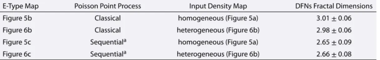
Table 2. DFN Simulations Parameters for E-Types Generations
E-Type Map Poisson Point Process Input Density Map DFNs Fractal Dimensions
Figure 5b Classical homogeneous (Figure 5a) 3.01 ± 0.06
Figure 6b Classical heterogeneous (Figure 6b) 2.98 ± 0.06
Figure 5c Sequentiala homogeneous (Figure 5a) 2.65 ± 0.09
Figure 6c Sequentiala heterogeneous (Figure 6b) 2.66 ± 0.08
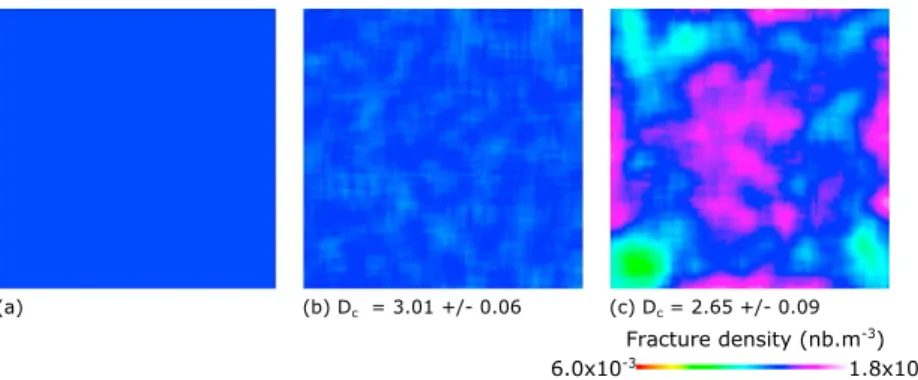
Figure 5. E types computed from 1000 realizations. (a) Homogeneous reference maps used. (b) E type obtained
from classical Poisson point process that produces uncorrelated DFNs (Dcis the average fractal dimension of DFNs generated). (c) E-type map obtained from sequential Poisson point process that produces spatial correlations. It shows a moderate bias that is interpreted to be related to a border effect.
E-type map with an average value of 1.37 × 10⁻²center m−3and a standard deviation of 2.08 × 10⁻⁴m−3
(Figure 5b). The sequential seeding process also produces an E-type map almost uniform with an aver-age values of 1.37 × 10⁻²center m−3but with a higher standard deviation (1.30 × 10⁻³m−3, Figure 5c).
The higher standard deviation indicates that the convergence of E type is more difficult due to the clustering of each realization. The sequential process also introduces a small bias in the fracture repartition by simulat-ing more objects in the center of the volume. We tried to reduce the intensity factors from h = g = 100 to
h = g = 10. This increased the DFNs correlation dimension from 2.65 ± 0.09 to 2.78 ± 0.06. The E-type map
obtained in this case is still very close to the one presented in Figure 5c. Additional tests on larger Cartesian grids suggest that the acceptance/rejection process produces subtle edge effect, which could be further investigated.
We performed the same study with a heterogeneous density map (Figure 6a). The E-type map correspond-ing to a heterogeneous Poisson point process (Figure 6b) is correlated to input density. The linear correlation coefficient linking the two properties is equal to 0.98. Note that producing DFNs that follow a heteroge-neous spatial repartition does not create significant spatial correlations between objects (Dc≈ 3). The E type obtained by mapping correlated DFNs (Dc= 2.66) is correlated to the reference map but with a lower coefficient (0.76, Figure 6c). As in the homogeneous case, we note a border effect that biases the global frac-ture repartition. It seems that objects are more likely to be simulated at the center of the volume. Reducing the intensity factors from h = g = 100 to h = g = 10 increases the DFNs correlation dimension to Dc= 2.79, reduces spatial correlations, and increases the correlation factor between the reference map and E-type map to 0.85. Because the intensity of spatial correlations may depend on the parameters of the sequential seeding process, we propose a sensitivity analysis in section 3.
Figure 6. E types computed from 1000 realizations. (a) Heterogeneous reference maps used. (b) E types obtained
from classical Poisson point process that produces uncorrelated DFNs (Dcis the average fractal dimension of DFNs generated). (c) E-type map obtained from sequential Poisson point process that produces spatial correlations.
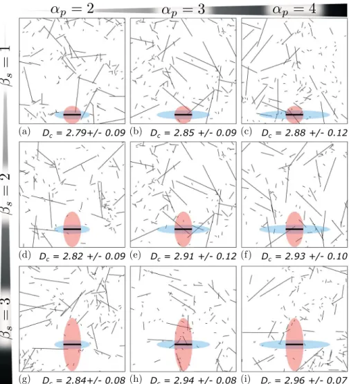
Figure 7. Sensitivity study on the fracture geomechanical model geometry factors. (a–i) Several models have been
tested and associated to their average correlation dimension. Increasing the size of shadow or stress concentration zone dilutes the impact of the sequential process and progressively produces nonfractal geometries.
3. Sensitivity Analysis on the Sequential Poisson Point Process
The parameters of the method are (1) the relative extents of stress concentration zone (𝛼p and 𝛽p), (2) the relative extents of the shadow zone (𝛼s and 𝛽s), (3) the intensity factors (g and h, equation (1)), and (4) the number of seeding sequences (s). All these parameters relate to the mechanical parameters of the rock, but no direct or statistical relationships have yet been established. This sensitivity study aims at quantifying the relationships between input parameters and spatial correlations in DFNs.
Simulations are performed with similar parameters as in section 2.3:
1. Simulations are performed on a Cartesian grid with 90 × 90 × 90 cubic voxels. 2. Fracture seeding uses a uniform density map generating 10,000 fractures.
3. The distribution law describing the fracture length follows a truncated power law with an exponent of 1.8 and values bounded between 1 and 30 m.
4. Fracture dip and strike are randomly selected in [0∘, 90∘] and [0∘, 360∘], respectively.
In this section, we describe and quantify the impact of both the geomechanical model and the chronological settings on the DFNs spatial correlations. The results of this sensitivity analysis are plotted in Figures 7, 8, and 11 and discussed in the next sections. For each set of tested parameters, we show a 2-D section of a 3-D DFN (red section, Figures 3 and 4). For each cases, we associate an average estimation of the correlation dimension computed over 100 realizations using the method described in section 2.3.
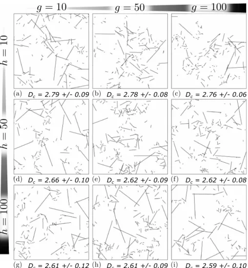
Figure 8. (a–i) Sensitivity on the intensity factors g and h (section 2.2). The global behavior tends to decrease Dc (increase spatial correlations) with the increase of h and g.
3.1. Sensitivity Study on Geomechanical Model Geometry Factors
To test the sensitivity of the method, we simulated 10,000 fractures in the same domain as in previous tests, by implanting 10 fractures per sequence (0.1% of the final DFN). We have varied the extent of stress concentration and shadow zones changing the values of 𝛽s and 𝛼p in the range [1–3] and [2–4], respectively, while keeping the other input factors constant (𝛽p = 1, 𝛼s = 0.5, and intensity factors g = h = 10).
The sensitivity analysis shows that the increase of shadow or stress concentration zone extents increases the correlation dimension of DFNs produced. In spite of the relatively large standard deviation of the correlation dimension, we observe a progressive dilution of spatial correlations from the clustered DFN (Figure 7a) to the uncorrelated DFN (Figure 7i).
3.2. Sensitivity Study on the Geomechanical Model Intensity Factors
In this sequence, we use the same chronology as in section 3.1 (0.1% of the DFN is simulated per sequence). One hundred simulations have been run using the geometric parameters described in Figure 1 (𝛼s = 𝛽s = 1, 𝛼p = 2 and 𝛽p = 0.5). The intensity factors in the stress concentration and shadow zones (g and h) vary between 10 and 100.
Results show a progressive decrease of the fractal dimension from Dc = 2.79 (Figure 8a) to Dc = 2.58 (Figure 8i) when g and h increase. Figure 8 also suggests that the impact of g is not as significant as the impact of h. We note a strong variation in the correlation dimension when we increase the value of h from 10
Figure 9. Evolution of the fractal dimension of DFNs with the intensity factor of the simplified geomechanical model.
Each triangle in grey corresponds to the correlation dimension computed on 100 DFN realizations for several values ofhandg = 10. In black, each point corresponds to the correlation dimension computed on 100 DFNs realizations for several values ofgandh = 10. Uncertainties are quite important, but we propose to identify a model to describe the evolution ofDc(h)(grey line) and the evolution ofDc(g)(black line).
(Dc= 2.8, Figures 8a–8c) to 50 (Dc= 2.6, Figures 8d–8f). Several other simulations have been made in order
to better characterize this trend (Figure 9).
More quantitatively, we found that the correlation dimension Dcmainly varies as a function of h (for g = 10) following the experimental model:
Dc(h) ≈ −0.18 log h + 2.96 ± 0.09 (3)
The correlation dimension Dc, however, is a quasi-constant function of g. Considering h = 10, the experimen-tal model of Dc(g) is described by
Dc(g) ≈ −0.03 log(g) + 2.81 ± 0.09 (4)
The low impact of the parameter g can be explained because the correlation dimension is a parameter that quantifies the spacing between fracture centers. Because g mainly attracts small fractures at the tip of larger ones, it affects very marginally the distance between fracture centers. Does this finding hold in the case of preferential fracture orientation? To answer that question, we repeated this study in the case of single set DFNs. Preferential fracture orientation does not change the behavior of Dc(h) because we used an isotropic shadow zone model. Then we focused on the Dc(g) and established the following experimental model:
Dc(g) ≈ −0.05 log(g) + 2.83 ± 0.08 (5)
The similarity between equations (4) and (5) suggests that the relation between the correlation dimension Dc and the intensity factors g and h is marginally affected by the orientation distribution of the fracture set. 3.3. Sensitivity Study on the Fracture Seeding Chronology
Theoretically, an idealized simulation should generate fractures one by one to take into account the impact of every newly simulated fracture in further simulation steps. In practice, simulating only one fracture per sequence is time consuming. For example, in our implementation on an Intel(R) Core(TM) i7-2600 CPU at 3.4 GHz, building a DFN with 10,000 fractures takes only few seconds when done in one sequence; but it takes approximately 10 min when simulating fractures 10 at a time. In our simulation method, the proportion of fractures that are simulated per sequence p varies with the total number of sequences (s) following:
p(s) =100
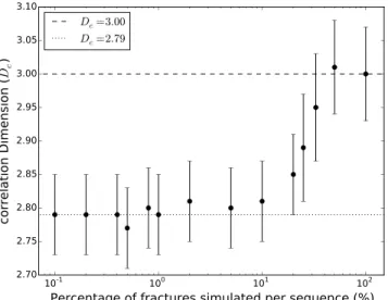
Figure 10. Fractal dimension versus proportion of DFN simulated per sequence. Correlation dimension of 2.8 is
obtained when 10% or less of the fracture network is simulated per sequence. Then, in the context of our example, a more robust result is obtained as soon as 0.4% of the fracture network is simulated per sequence.
This means that for high values of s, we need a strong increase of s to observe only a small decrease of p(s). A high increase of s leads to a high increase of the computation time. The current section aims at testing the sensitivity of the method concerning the chronological seeding of fractures.
For this analysis, we simulated 10,000 fractures with a number of sequences (s) that vary between 1 and 1000 (Figure 10). Simulations have been done using the parameters summarized in Table 3.
The results suggest that simulating 10% of fractures at each sequence is sufficient to converge to a constant correlation dimension (Dc). Furthermore, the value of Dc stabilizes as soon as 0.4% of the DFN is simulated at each sequence. Another result of the sensitivity analysis is that several DFNs may have the same correla-tion dimension but different spatial organizacorrela-tions (Figure 11). In other words, the hierarchical organizacorrela-tion of small fractures that clustered around largest fracture tips may not be described by Dc. Indeed, the correlation dimension only quantifies the clustering of fracture centers and does not quantify the position of fractures according to their size. Figure 11 shows the organization of fracture traces obtained with various number of sequences. An increase of the number of sequences seems to cluster small fractures at large fracture tips and also seems to decrease the number of X-shaped contacts. This may have an impact on the DFNs connectivity that we propose to study in section 4.
4. Impact of the Sequential Poisson Point Process on 3-D DFNs Connectivity
Connectivity is a key property of fracture networks because it is directly linked to physical behavior of frac-tured rocks. Numerous studies have used percolation theory to characterize flow and transport in porous and fractured media (see Berkowitz and Balberg [1993] and Berkowitz [2002] for reviews). In this section, we inves-tigate the DFN percolation threshold and local connectivity model that emerge from the sequential Poisson point process. We describe and quantify the impact of spatial correlations and more generally the impact of the chronological seeding of fractures on percolation properties in the isotropic case.
Table 3. Input Parameters for Sequential DFN Simulations Used in
Sections 3.3 and 4
Fracture Impact Model W Extent UV Extent Intensity Factor
Shadow zone 𝛽s= 1 𝛼s= 1 h = 10
Figure 11. Sensitivity on the number of sequences on the sequential seeding process. (a–c) Simulated in 1000, 100,
and 10 sequences; it means that 0.1%, 1%, and 10%, respectively, of the fracture network have been simulated per sequence. Whereas the correlation dimension is comparable (2.8), we note some differences in the global organization (X-shapes, hierarchy). This impact is quantified in section 4.
We propose a statistical analysis over 1000 3-D DFNs that are simulated considering the following parameters. 1. The 30 × 30 × 30 cells Cartesian grid sets the scale of the study and provides a uniform prior fracture
density map.
2. Fracture strike and dip follow a uniform distribution.
3. Power law fracture length distribution is defined as follows: n(l) = l−a; l ∈ [1, 30].
Darcel [2003] shows that the connectivity at percolation is mainly driven by the largest fractures and not by spatial correlations for fracture networks with a small power law exponent (a ≈ 1). A larger power law exponent increases the proportion of small fractures in the network; then spatial correlations may have a stronger impact on the percolation study. Therefore, we chose to study the impact of sequential seeding process on the connectivity of DFN of power law exponent a = 3. The sequential seeding process uses the parameters described in Table 3. We made the proportion of fractures simulated at each sequence (p(s), section 3.3) varying in the following range: (1) p(s) = 100% (equivalent to the classical Poisson point process), (2) p(s) = 10%, (3) p(s) = 1%, and (4) p(s) = 0.1%.
During the simulation process, the uniform fracture density was progressively increased until the percolation state would be reached. The percolation state is characterized when a cluster of fractures gets through the whole volume of rock. It means that each of the six faces of the volume has to be intersected by the percolating cluster (Figure 12).
Figure 12. The 3-D DFNs realizations at percolation state for extreme investigated cases. (a) Geometry of percolation
DFN obtained simulating all fractures in the same sequence. (b) Geometry of percolation DFN obtained simulating 0.1% of the fractures at each sequence. Percolating clusters are shown in red.
Figure 13. Impact of sequential seeding on the percolation threshold. It describes the probability for DFNs to percolate
as a function of the percolation factor (pf ). This experiment shows that the percolation threshold decreases with the proportion of fractures initiated at each sequence.
4.1. The Percolation Parameter
Many studies have been made to identify a parameter that presents an invariant threshold that characterizes the percolation state of fracture networks. Robinson [1983, 1984] first linked the percolation parameters to the fracture density in the case of unit length fracture randomly distributed and randomly oriented in 2-D space. He found that the average number of intersection per fracture describes the percolation independent of the fracture orientation distribution law. Balberg et al. [1984] investigated the estimation of the excluded volume around every fracture in a network. The excluded volume is the average volume surrounding an object into which the center of another object cannot lie without intersecting it. This work allows to define a very general expression of a factor describing the percolation of 3-D fracture networks. Finally, Bour and Davy [1997, 1998] and De Dreuzy et al. [2000] defined the percolation factor, pf , for planar fractures as
pf = ( n ∑ i=1 < l3 i > ) ∕V (7)
where n is the number of fractures in the fracture network, < li3 > is the third moment of the length distribution law, and V is the considered volume of rock.
We generated 1000 percolating DFNs for each of the four different sequential seeding processes previously described. Figure 13 shows the probability for these DFNs to percolate against the percolation factor. We observe that the percolation threshold decreases when we decrease the proportion of fractures simulated at each seeding sequence (p(s), Figure 13). This corroborates the findings of Darcel [2003] that spatial correla-tions impact the connectivity and the percolation threshold (for networks with a high power law exponent). We observe here that the sequential seeding process creates spatial correlations that can be measured by the correlation dimension Dc and allows DFNs to reach the percolation state with a smaller factor pf as compared to uncorrelated DFNs. We also show that the sequential process may create DFNs with a hierarchical organiza-tion (secorganiza-tion 3.3) that cannot be discriminated by the correlaorganiza-tion dimension (Dc = 2.8 for p(s) = 0.1, 1, or 10) but still reduces the percolation threshold. This is probably due to the local organization of fractures induced by the process.
4.2. Average Number of Intersections Per Fracture
This section investigates the local connectivity of DFNs simulated in section 4.1. The average number of inter-sections per fracture normalized by the fracture intensity (P32: fracture area per unit volume in m2 m−3) has
Figure 14. Impact of the proportion of fractures simulated per sequence (p(s)) on the average number of intersections per fracture. Uncorrelated DFNs follow a simple power law model that only depends on the fracture length (black line model). Spatial correlations between fractures are obtained by reducing the proportion of fractures simulated per sequence and quantified by the correlation dimension (Dc). It impacts the connectivity model by (1) increasing the number of intersections for small fractures and (2) reducing it for large ones. Reducing the proportion of fractures (p(s)) simulated at each sequence allows to better capture the behaviors of the transition scale (even if the correlation dimension does not change).
Simulating all fractures in the same sequence produces fracture networks where the number of intersections per fracture increases with their length. For such DFNs, where fractures are randomly and independently sim-ulated, the local connectivity model follows a single power law model (black line, Figure 14). Decreasing the number of fractures simulated at each sequence changes the global organization of fractures and modifies the model describing the local connectivity. Also, the number of intersections between small objects tends to increase, whereas it decreases for large ones (Figure 14). It seems to naturally reproduce the two fractur-ing regimes described by Wu and Pollard [1995], Josnin et al. [2002], and Davy et al. [2010]. The early initiation of fractures appears in a poorly fractured network. It leads to little interactions with other objects that create large fractures with few connections (large fractures are simulated first). The progressive apparition of addi-tional fractures intensifies the interactions between objects and increases the number of intersections per object. This explains why small fractures, which appear when the fracture network is well developed, have relatively more intersections.
Figure 14 shows how progressive the fracture apparition should be to observe a smooth transition from the poorly to the well-developed fracturing regime. If the number of fractures simulated per sequence (p(s)) is too high, then a discontinuity appears in the local connectivity model (dotted lines, Figure 14). In such cases, the local connectivity model of medium fractures follows the same model as the one observed for uncorrelated fracture networks. The best way to capture the behavior of the transition scale and to mimic the actual fracturing process would be to simulate the fractures one by one. However, simulating 0.1% of fractures per sequence is much more efficient and gives a good idea of the continuous local connectivity model.
5. Discussion and Conclusion
The presented method uses a stochastic, sequential, and nonstationary nucleation process to simulate hier-archical and spatially correlated DFNs. It is not only conditioned by statistics that characterize the natural fracture network geometry but also use rules inspired from mechanical concepts to progressively seed frac-tures in a 3-D model. As compared to the “likely Universal Fracture Model” [Davy et al., 2010, 2013] that randomly nucleates and propagates fractures until their length is statistically equal to the distance to the nearest fracture, we individualize a shadow zone and a stress concentration zone in order to drive the progressive fracture nucleation process. Large fractures, simulated first, organize the nucleation of later fractures.
We show that such a chronological fracture seeding produces a hierarchical organization of fractures that leads to correlated networks. Reducing the proportion of fractures simulated at each sequence likely gets closer to the natural fracturing process and intensifies the spatial correlations between fractures. We iden-tify a threshold proportion of fractures simulated at each sequence from which the estimated correlation dimension stops changing (section 3.3). This value is experimental and probably depends on parameter set-tings selected in this study. The computed correlation dimension does not completely capture the spatial features of the simulated networks. Further study needs to investigate a new measure of spatial correlations that take into account the anisotropy in the positioning of fracture center. Indeed, the correlation dimension (equation (2)) describes the organization of fracture centers and does not fully describe the hierarchical orga-nization of objects of various size. Decreasing the proportion of fractures simulated at each sequence tends to cluster small fractures at the tips of large ones. It visually decreases the number of X-shaped intersections that may be inconsistent according to the relative chronology of fracture growth (Figure 11). Section 4 shows that DFNs characterized by the same correlation dimension may have significant differences in their local connec-tivity model due to their spatial organization. The best case would be to consider every fracture previously simulated in the current fracture simulation. However, it would lead to impractically feasible computational costs for large 3-D simulation domains.
Spacing and clustering of DFN are important aspects that impact the connectivity of the network. Masihi and King [2007] proposed a calibration process based on the minimization of the elastic energy dissipated by frac-tures. They suggest that such optimized networks present a positive correlation between the length and the spacing of objects, and they show that the global organization of fractures has an impact on the percola-tion threshold. Our sequential parent-daughter Poisson point process tends to impose a similar organizapercola-tion by defining shadow zone extents proportionally to fracture size. We have shown that our fracture simulation strategy significantly impacts DFN properties at percolation (section 4). The sequential seeding produces hier-archical DFNs that favor fracture connections and produce clusters. It allows to reach the percolation with a reduced percolation threshold compared to classical Poisson simulations. The main limitation of the method is that we simulate fractures in their final state and we neglect mechanical interactions and fracture nucle-ation during the growth. This simplificnucle-ation reduces the complex geometry of fractures that result from the growth and coalescence processes into planar objects. These can lead to an underestimation of the network connectivity. Further studies should take into account an efficient model to reproduce the fracture growth and initiation during the growth by considering ramified and curved objects [Gringarten, 1998; Srivastava et al., 2005; Bonneau et al., 2013]. Incorporating curved fractures in the simulation process could have an additional effect on connectivity properties. Generating realistic geometry for nonplanar fracture intersections in 3-D is an issue hardly discussed in the literature. But, because the proposed method impacts the relative position of fractures according to mechanical considerations, it may facilitate the representation of such 3-D branching contacts.
The hierarchy and the spatial correlation of fractures in DFNs are set by the mechanical model associated to each fracture. We propose parameters that describe a symmetrical shape that roughly approximates the first-order stress anomalies around fractures. Such a parametrization needs to be simple in order to keep the simulation computationally efficient. It would be interesting to investigate other shapes in order to reflect the asymmetry of stress concentration near sliding fracture tips [Kim et al., 2004] or to use explicit mechanical models [Paluszny and Zimmerman, 2013]. In the same spirit, new rules may be implemented in order to impose spatial correlation on neighboring fracture orientations. This could be suitable to produce “wing-crack” struc-tures often observed in nature. More generally, a comparison between simulated DFNs and independent data (field, analogs) would be a valuable work to validate the simulation method. In this study, we modified the parameters that set the stress concentration zone (or respectively the shadow zone) extent and inten-sity to quantify their impact on the fractal dimension of DFN models (section 3). However, statistics on the fractal dimension that emerges from hundred realizations show a relatively large standard deviation. As a con-sequence, it seems difficult to constrain precisely the expected correlation dimension according to natural network characterization. The shadow zone intensity factor (h) is the parameter that most impacts the value of the emerging fractal dimension. An experimental model that links the value of the fractal dimension to the value of h has been identified (section 3.2). This model is an interesting tool to set practically the fractal dimen-sion for output DFNs. Further work has to be done in order to better understand this emerging behavior and relate it to the physical fracturing process.
Appendix A: Sequential Seeding Process Algorithm
References
Balberg, I., C. H. Anderson, S. Alexander, and N. Wagner (1984), Excluded volume and its relation to the onset of percolation, Phys. Rev. B:
Condens. Matter, 30, 3933–3943, doi:10.1103/PhysRevB.30.3933.
Berkowitz, B. (2002), Characterizing flow and transport in fractured geological media: A review, Adv. Water Resour., 25, 861–884. Berkowitz, B., and I. Balberg (1993), Percolation theory and its application to groundwater hydrology, Water Resour. Res., 29(4), 775–794. Bonneau, F., V. Henrion, G. Caumon, P. Renard, and J. Sausse (2013), A methodology for pseudo-genetic stochastic modeling of discrete
fracture networks, Comput. Geosci., 56, 12–22.
Bonnet, E., O. Bour, N. Odling, P. Davy, I. Main, P. Cowie, and B. Berkowitz (2001), Scaling of fracture systems in geological media, Rev.
Geophys., 39(3), 347–383.
Bour, O., and P. Davy (1997), Connectivity of random fault networks following a power law fault length distribution, Water Resour. Res., 33, 1567–1583.
Bour, O., and P. Davy (1998), On the connectivity of three-dimensional fault networks, Water Resour. Res., 34(10), 2611–2622. Bour, O., and P. Davy (1999), Clustering and size distributions of fault patterns: Theory and measurements, Geophys. Res. Lett., 26(13),
2001–2004.
Bour, O., P. Davy, C. Darcel, and N. Odling (2002), A statistical scaling model for fracture network geometry, with validation on a multiscale mapping of a joint network (Hornelen Basin, Norway), J. Geophys. Res., 107( B6), 2113, doi:10.1029/2001JB000176.
Cacas, M.-C., J.-M. Daniel, and J. Letouzey (2001), Nested geological modelling of naturally fractured reservoirs, Pet. Geosci., 7, 43–52. Chilès, J.-P. (2005), Stochastic modeling of natural fractured media: A review, in Geostatistics Banff 2004, Quantitative Geology and
Geostatistics, vol. 14–1, edited by O. Leuangthong and C. V. Deutsch, pp. 285–294, Springer, Netherlands, doi:10.1007/978-1-4020-3610-1_29.
Chilès, J. (1988), Fractal and geostatistical methods for modeling of a fracture network, Math. Geol., 20(6), 631–654, doi:10.1007/BF00890581.
Cladouhos, T. T., and R. Marrett (1996), Are fault growth and linkage models consistent with power-law distributions of fault lengths?,
J. Struct. Geol., 18(2–3), 281–293, doi:10.1016/S0191-8141(96)80050-2.
Cosgrove, J. W., and T. Engelder (2004), The Initiation, Propagation, and Arrest of Joints and Other Fractures, vol. 231, Special Publ., Geological Society, London.
Darcel, C. (2003), Corrélations dans les réseaux de fractures: Caractérisation et conséquences sur les propriétés hydrauliques, PhD. thesis, Univ. de Rennes 1, Rennes, France.
Darcel, C., O. Bour, and P. Davy (2003), Cross-correlation between length and position in real fracture networks, Geophys. Res. Lett., 30(12), 1650–1653, doi:10.1029/2003GL017174.
Davy, P., A. Sornette, and D. Sornette (1990), Some consequences of a proposed fractal nature of continental faulting, Nature, 348(6296), 56–58.
Davy, P., et al. (2010), A likely universal model of fracture scaling and its consequence for crustal hydromechanics, J. Geophys. Res., 115, B10411, doi:10.1029/2009JB007043.
Davy, P., R. Le Goc, and C. Darcel (2013), A model of fracture nucleation, growth and arrest, and consequences for fracture density and scaling, J. Geophys. Res. Solid Earth, 118(4), 1393–1407, doi:10.1002/jgrb.50120.
Acknowledgments
The authors are grateful to the academic and industrial sponsors of the RING-Gocad Consortium managed by ASGA (Association Scientifique pour la Géologie et ses Applications) for funding this work, and to Paradigm Geophysical for providing the Gocad software and API. We would also like to thank Philippe Davy and all reviewers for constructive comments which helped improve this paper. This work was performed in the frame of the “Investissements d’avenir” Labex RESSOURCES21 (ANR-10-LABX-21). The data for this paper are available by contacting the corresponding author at francois.bonneau@univ-lorraine.fr.
De Dreuzy, J., P. Davy, and O. Bour (2001), Hydraulic properties of two-dimensional random fracture networks following a power law length distribution: 2. Permeability of networks based on lognormal distribution of apertures, Water Resour. Res., 37(8), 2079–2095.
De Dreuzy, J.-R., P. Davy, O. Bour, and et al. (2000), Percolation parameter and percolation-threshold estimates for 3D random ellipses with widely-scattered distributions of eccentricity and size, Phys. Rev. E: Stat. Nonlinear Soft Matter Phys., 62(5), 5948–5952.
De Dreuzy, J.-R., G. Pichot, B. Poirriez, and J. Erhel (2013), Synthetic benchmark for modeling flow in 3D fractured media, Comput. Geosci., 50, 59–71.
Dershowitz, W., P. La Pointe, and T. Doe (2004), Advances in discrete fracture network modeling, in Proceedings of the U.S. EPA/NGWA
Fractured Rock Conference, pp. 882–894, U.S. EPA/NGWA (National Ground Water Association), Portland, Maine.
Dowd, P. A., C. Xu, K. V. Mardia, and R. J. Fowell (2007), A comparison of methods for the stochastic simulation of rock fractures, Math. Geol.,
39(7), 697–714.
Griffith, A. (1921), The phenomena of rupture and flow in solids, Philos. Trans. R. Soc. London, Ser. A, 221, 163–198.
Griffith, A. (1924), The theory of rupture, in Proceedings of the First International Conference for Applied Mechanics, pp. 55–63, Technische Boekhandel en Drukkerij J. Waltman Jr., Delft, Netherlands.
Gringarten, E. (1998), FRACNET: Stochastic simulation of fractures in layered systems, Comput. Geosci., 24( 8), 729–736.
Jing, L. (2003), A review of techniques, advances and outstanding issues in numerical modelling for rock mechanics and rock engineering,
Int. J. Rock Mech. Min. Sci., 40, 283–353.
Josnin, J.-Y., H. Jourde, P. Fnart, and P. Bidaux (2002), A three-dimensional model to simulate joint networks in layered rocks, Can. J. Earth Sci.,
39(10), 1443–1455, doi:10.1139/e02-043.
Journel, A. G. (1983), Nonparametric estimation of spatial distributions, J. Int. Assoc. Math. Geol., 15(3), 445–468. Kim, Y.-S., D. Peacock, and D. Sanderson (2004), Fault damage zones, J. Struct. Geol., 26, 503–517.
Lamarche, J., A. P. Lavenu, B. D. Gauthier, Y. Guglielmi, and O. Jayet (2012), Relationships between fracture patterns, geodynamics and mechanical stratigraphy in carbonates (South-East Basin, France),Tectonophysics, 581, 231–245.
Lantuéjoul, C. (2002), Geostatistical Simulation: Models and Algorithms, Springer, Berlin, Germany. Lyakhovsky, V. (2001), Scaling of fracture length and distributed damage, Geophys. J. Int., 144(1), 114–122.
Mace, L., P. Muron, and J.-L. Mallet (2005), Integration of fracture data into 3D geomechanical modeling to enhance fractured reservoirs characterization, in Proceedings of the SPE Annual Technical Conference and Exhibition, pp. 1–9, Soc. Pet. Eng., Dallas, Tex.
Mandelbrot, B. (1983), The Fractal Geometry of Nature, Freeman, 468 pp., New York.
Masihi, M., and P. R. King (2007), A correlated fracture network: Modeling and percolation properties, Water Resour. Res., 43, W07439, doi:10.1029/2006WR005331.
Odling, N. E., and I. Webman (1991), A conductance mesh approach to the permeability of natural and simulated fracture patterns, Water
Resour. Res., 27(10), 2633–2643.
Olson, J. (1993), Joint pattern development: Effects of subcritical crack growth and mechanical crack interaction, J. Geophys. Res., 98(B7), 12,251–12,265.
Ouillon, G., C. Castaing, and D. Sornette (1996), Hierarchical geometry of faulting, J. Geophys. Res., 101( B3), 5477–5487.
Paluszny, A., and R. W. Zimmerman (2013), Numerical fracture growth modeling using smooth surface geometric deformation, Eng. Fract.
Mech., 108, 19–36.
Pollard, D., and A. Aydin (1988), Progress in understanding jointing over the past century, Geol. Soc. Am. Bull., 100, 1181–1204. Renshaw, C. E., and D. D. Pollard (1994), Numerical simulation of fracture set formation: A fracture mechanics model consistent with
experimental observations, J. Geophys. Res., 99, 9359–9372.
Robinson, P. (1984), Numerical calculations of critical densities for lines and planes, J. Phys. A: Math. Gen., 17, 28–23. Robinson, P. C. (1983), Connectivity of fracture systems—A percolation theory approach, J. Phys. A: Math. Gen., 16(3), 605–614.
Rodriguez-Herrera, A., et al. (2015), Stress-induced signatures in 4D seismic data: Evidence of overburden stress arching, in 2015 SEG Annual
Meeting, pp. 5368–5372, Society of Exploration Geophysicists, New Orleans, La.
Sayers, C. M. (2009), Seismic characterization of reservoirs containing multiple fracture sets, Geophys. Prospect., 57(2), 187–192, doi:10.1111/j.1365-2478.2008.00766.x.
Serrano, I., F. Torcal, and J. Morales (2014), Distribution of crack density parameter in Central Betic Cordillera (Southern Spain), Geophys. J.
Int., 196(1), 22–33.
Srivastava, R., P. Frykman, and M. Jensen (2005), Geostatistical simulation of fracture networks, in Geostatistics Banff 2004, Quantitative
Geology and Geostatistics, vol. 14–1, edited by R. Srivastava, P. Frykman, and M. Jensen, pp. 295–304, Springer, Netherlands.
Stoyan, D., and H. Stoyan (1994), Fractals, Random Shapes and Point Fields, Wiley, New York.
Swaby, P. A., and K. D. Rawnsley (1996), An interactive 3D fracture modelling environment, in SPE-36004-MS, pp. 82–87, Society of Petroleum Engineers, Dallas, Tex., doi:10.2118/36004-MS.
Tuckwell, G., L. Lonergan, and R. Jolly (2003), The control of stress history and flaw distribution on the evolution of polygonal fracture networks, J. Struct. Geol., 25(8), 1241–1250.
Velde, B., J. Dubois, D. Moore, and G. Touchard (1991), Fractal patterns of fractures in granites, Earth Planet. Sci. Lett., 104(1), 25–35. Welch, J., R. Davies, R. Knipe, and C. Tueckmantel (2009), A dynamic model for fault nucleation and propagation in mechanically layered
section, Tectonophysics, 474, 473–492.
Wu, H., and D. D. Pollard (1995), An experimental study of the relationship between joint spacing and layer thickness, J. Struct. Geol., 17(6), 887–905, doi:10.1016/0191-8141(94)00099-L.
Xu, C., and P. Dowd (2010), A new computer code for discrete fracture network modelling, Comput. Geosci., 36(3), 292–301, doi:10.1016/j.cageo.2009.05.012.
Yamaji, A., and K. Sato (2011), Clustering of fracture orientations using a mixed Bingham distribution and its application to paleostress analysis from dike or vein orientations, J. Struct. Geol., 33(7), 1148–1157.