Discount bundling via dense product embeddings
by
Madhav Kumar
M.Sc. Economics
IGIDR, 2011
B.Sc. (Hons.) Physics
University of Delhi, 2008
Submitted to the Department of Management
in partial fulfillment of the requirements for the degree of
Master of Science in Management Research
at the
MASSACHUSETTS INSTITUTE OF TECHNOLOGY
May 2020
c
○ Massachusetts Institute of Technology 2020. All rights reserved.
Author . . . .
Department of Management
April 28, 2020
Certified by . . . .
Sinan Aral
David Austin Professor of Management
Professor, Information Technology and Marketing
Thesis Supervisor
Accepted by . . . .
Catherine Tucker
Sloan Distinguished Professor of Management
Professor of Marketing
Chair, MIT Sloan PhD Program
Discount bundling via dense product embeddings
by
Madhav Kumar
Submitted to the Department of Management on April 28, 2020, in partial fulfillment of the
requirements for the degree of
Master of Science in Management Research
Abstract
Bundling, the practice of jointly selling two or more products at a discount, is a widely used strategy in industry and a well examined concept in academia. Historically, the focus has been on theoretical studies in the context of monopolistic firms and assumed product relationships, e.g., complementarity in usage. We develop a new machine-learning-driven methodology for designing bundles in a large-scale, cross-category retail setting. We leverage historical purchases and consideration sets created from clickstream data to generate dense continuous representations of products called embeddings. We then put minimal structure on these embeddings and develop heuristics for complementarity and substitutability among products. Subsequently, we use the heuristics to create multiple bundles for each product and test their performance using a field experiment with a large retailer. We combine the results from the experiment with product embeddings using a hierarchical model that maps bundle features to their purchase likelihood, as measured by the add-to-cart rate. We find that our embeddings-based heuristics are strong predictors of bundle success, robust across product categories, and generalize well to the retailer’s entire assortment.
Thesis Supervisor: Sinan Aral
Title: David Austin Professor of Management Professor, Information Technology and Marketing
1. Introduction
Bundling is a widespread product and promotion strategy used in a variety of settings such as fast food (meal + drinks), telecommunications (voice + data plan), cable (tv + broadband) and insurance (car + home insurance). Given its pervasiveness, it has received considerable attention with over six decades of research analyzing conditions under which it is profitable, the benefits of different bundling strategies, and its welfare consequences. However, in spite of the vast literature, there is little empirical guidance for retailers on how to create good promotional bundles. For example, consider a medium sized online retailer with an inventory of 100,000 products across multiple categories. Which two products should the retailer use to form discount bundles? There are (︀1025)︀ ≈ 50 million combinations. Conditional on selecting a candidate product, there are 99,999 options to choose from to make a bundle. Is there a principled way that the managers can use to select products to form many bundles?
In this study, we offer a new perspective to the bundle design process which leverages historical consumer purchases and browsing sessions. We use them to generate latent dense vector representations of products in such a way that proximity of two products in this latent space is indicative of “similarity” among those products. A key insight in our method is the distinction between the representation of product purchases and representation of consideration sets, where consideration sets include the products that were viewed together but not purchased together. We posit that products that are frequently bought together tend to be more complementary whereas products that are frequently viewed but not purchased together tend to be more substitutable. Then, depending on whether the products were frequently co-purchased or co-viewed (but not purchased), the degree similarity in the latent space is suggestive of complementarity or substitutability respectively. We put minimal structure on this latent-space-based contextual similarity to generate product bundles. We then learn consumers’ preferences over these suggested bundles using a field experiment with a large U.S.-based online retailer. Finally, we generalize our findings to the entire product assort-ment of the retailer by modeling the bundle success likelihood, as measured by the bundle add-to-cart rate, as a function of the product embeddings using hierarchical logistic regression.
Much of the earlier work on bundling was from economists seeking conditions under which a monopolist might choose to sell its products as independent components vs. pure bundles vs. mixed bundles (Adams and Yellen,1976;Schmalensee,1982;Venkatesh and Kamakura,2003). These earlier papers were motivated by considerations of price discrimination and hinged on analytical models that rely on pre-specified product complementarity and substitutability, or an ex-ante well-defined underlying relationship between the products. For instance, Adams and Yellen (1976) conduct their analysis by assuming that the products have independent demands, Venkatesh and Kamakura (2003) provide conditions for products that are assumed to be either complements or substitutes, and, more recently, Derdenger and Kumar (2013) develop their model in the context of video-games and consider obvious complements in usage — consoles and games. Furthermore, most studies work with the idea that a single firm is producing the goods, bundling them together, and then selling them at the discounted price. However, a more realistic picture — and the one we consider in this study — is one of a downstream retailer bundling products from different firms.
Our work enhances the existing literature on bundling in economics and marketing in three ways. First, instead of considering pre-defined relationships among products, we generate continuous metrics that are heuristics for the degree of complementarity and substitutability based on historical consumer purchases and consideration sets. A major strength of our approach is that we can learn relationships between two products which may have never been co-purchased or co-viewed together but still be strongly related to each other. This permits us to develop an effective bundle design strategy in a large-scale cross-category retail setting where co-purchases are sparse, a relatively unexplored context in bundling studies. Second, we test the effectiveness of our methodology by running a field-experiment with a large online retailer in the US, providing empirical color to a largely theoretical literature. Third, we explore the idea of generating bundles from imperfect substitutes to tap into the variety-seeking behavior of consumers, which we call variety bundles.
This thesis also provides implementable insights for managers. Identifying the best bundles for a retailer with an assortment of a 100,000 products involves considering an action space with millions of potential bundles, a combinatorially challenging task. Our methodology allows us to filter this action space in a principled data-driven way using machine-learning based heuristics, providing substantial efficiency gains while accounting for consumer preferences. For example, some of the bundles created by category managers include different volumes of the Harry Potter book series, branded sports team gear (hand towel and bath towel), and
same-brand shampoo and conditioner. Our approach adds several types of bundles to this set: cross-category complements with mouthwash and deodorant, within-category complements involving laundry detergent and stain remover, and variety snacks with potato chips and animal crackers. Moreover, since we run the experiment at a product level, we are able to flexibly generate micro-level insights, e.g., which brands make good bundles, as well as high-level insights such as which categories make good bundles.
The thesis is structured as follows. Literature review is in the next section. The model is described in Section 3, which is followed by a description of the data and the product embeddings. The details of the field experiment are presented in Section 6 and the insights from predictive modeling are shown in Section 7. Section 8 concludes.
2. Literature review
Our study draws inspiration from two distinct strands of literature: the bundling literature from economics, marketing and operations research (OR), and the machine learning work from natural language processing (NLP).
Economics, marketing, and OR
The idea of bundling is described visually and intuitively by Adams and Yellen (1976), who show that bundling is profitable in the case of goods with independent demands because firms are able to sort consumers based on reservation prices, which in turn allows them to extract a larger portion of consumer surplus. Lewbel(1985) extendsAdams and Yellen(1976) to include interdependent demand and shows that it may not always be profitable to bundle complements. He goes further to explain that a multi-product monopolist may actually find it profitable to bundle imperfect substitutes by using mixed bundling. Schmalensee (1982) provides the conditions for pure bundling (selling products only as a bundle) and mixed bundling (selling products independently and as a bundle) in the case of a single-product monopolist and a competitively sold product as a function of reservation prices, production costs, and market structure. He finds the mixed bundling can be profitable when there is negative correlation between the reservations prices of the two goods. In a separate paper, Schmalensee (1984) attempts to generalize Adams and Yellen (1976)’s findings by assuming that the distribution of reservation prices is bivariate normal. With the Gaussian tool (and its caveats) in hand, he finds that with symmetric reservation price distribution, pure bundling is better than unbundled sales. Salinger(1995) uses the concept of negatively and positively correlated demand to show the welfare consequences and profitability of bundling graphically. His primary focus though is on the relationship between demand for the bundle and the demand for individual components of the bundle.1
1Stremersch and Tellis(2002) is an excellent introductory guide to the concept of bundling from a marketing
perspective and also provides generic conditions under which one form of bundling may be preferred over another.
Venkatesh and Kamakura (2003) consider a multi-product monopolist and build an analyt-ical model based on contingent values to identify conditions when bundling complements, substitutes, and independently valued products works. Venkatesh and Mahajan (1993) take a probabilistic approach to find conditions suitable for pure components, pure bundling or mixed bundling. They include time availability along with reservation price as another dimension for consumer evaluation and for each bundling strategy, calculate the optimal prices, profits, and market share. Ansari et al. (1996) extend their work by allowing the number of components to be endogenously determined. They apply their model to the non-profit space by studying survey data on classical music events.
While the setting in most economics papers has been a monopolist firm of some kind, a few papers in marketing have focused on the retail perspective as well. Mulhern and Leone (1991) consider retail pricing and develop a theoretical framework based on demand
inter-dependencies. They consider the case of multi-product pricing based on the notion that promotion pricing of related products is equivalent to implicit price bundling. Relationships are defined in such a way that products within a product line are substitutes and those across product-lines can be either substitutes, complements, or independent products. They then show how retailers can use price promotions using store-level weekly scanner data on cake mix and frosting. Chung and Rao (2003) build a multi-category choice model for bundles based on the attributes of the products. They estimate their parameters by pre-defining a set of physical features and attributes for personal computers. Although, their choice model does account for cross-category bundles and hence, heterogeneous components, their definition of categories is fairly narrow, with all products being complements in usage. Bhargava (2012) studies the impact of a merchant bundling products from different firms. The author builds an analytical model to find conditions under which pure bundling and pure components are profitable. He further shows that bundling may not be profitable due to vertical and horizontal channel conflicts unless the firms can co-ordinate on prices.
Among empirical works, Yang and Lai(2006) use association rules to create bundles of books based on shopping-cart data and browsing data. The find that these bundles are better, as measured by total number books bought, than the bundles based solely on order data or solely using browsing data. Although, Yang and Lai (2006)’s idea and our idea are similar in spirit, i.e., both use browsing and purchase data to generate bundles, our scopes are widely different - books vs. cross-category retail. Nevertheless, a key takeaway from their study is that they found incremental value in using browsing data in addition to purchase data in forming bundles, an idea that we leverage too.
Jiang et al.(2011) also study bundling in the context of an online retailer selling books and use non-linear mixed integer programming to recommend the next best product given what it is currently in the basket. They do numerical studies to show that their method leads to more customers purchasing discounted bundles as well as improved profits for the retailer. More recently, Derdenger and Kumar(2013) empirically test some of bundling theories described above in the context of hand-held video games. The investigate the options of pure bundling vs. mixed bundling along with the dynamic effects of bundling for durable complementary products. They find that mixed bundling leads to higher revenues than pure bundling or pure components. Bundling also causes consumers to behave strategically in that they lead certain segments of consumers to advance their purchases and certain segments to enter the market which they might not have in the absence of bundling.
To summarize, previous research has carefully examined the efficacy of different bundling strategies in a variety of settings with a multitude of tools such as graphical analysis, an-alytical frameworks, probabilistic, and structural models, survey-based empirical exercises, and modeling historical purchase data. Conclusions, though numerous, are contingent on the assumptions the researchers have made. Depending upon the context, researchers have found bundles of complementary, substitutes, and independent products to be profitable. With lessons from these papers as strong a foundation, our paper offers a new perspective to an old problem. We do not attempt to fill any “gap” in the literature but rather deliver a novel prescriptive methodology that is rooted in data, is empirically validated using a field experiment, and is practically implementable by managers and retailers.
Machine learning
We leverage techniques developed for analyzing large unstructured data, especially text data, in computer science called neural embeddings. The basic idea behind these methods is to convert textual representations of words to numerical vectorized representations which are dense and continuous (Mikolov et al.,2013a,b). Frequent co-occurrences of words within and across documents are indicative of semantic and syntactic relationships between them. Neural embeddings translate co-occurrence patterns in text into a latent space of a pre-specified dimension, say 𝒟, where proximity in the latent space implies semantic similarity. We don’t discuss the core literature here but rather focus on the applications of it in our domain. The interested reader can look at Mikolov et al. (2013a,b).
The concept of latent embeddings has been applied to diverse settings such as reviews, neural activity, movie ratings, product recommendations, and even market baskets (Rudolph et al., 2016, 2017;Ruiz et al.,2017; Barkan and Koenigstein, 2016; Timoshenko and Hauser, 2019). The core data framework in these papers is similar to ours, in which there is unstructured data of a sequence of objects generated through repeated actions of an agent. Those actions could be rating different movies by a viewer (Rudolph et al., 2016), or listening to songs (Barkan and Koenigstein, 2016), or purchasing multiple products together (Rudolph et al., 2016; Ruiz et al., 2017). Elaborating with the example of purchase baskets, the fundamental action in these scenarios is binary, i.e., purchasing a product or not, which can be thought of a word being present or not. A sequence of such binary activities (words) then makes up a sentence, which in our example is a product basket, and multiple product baskets constitute to form the entire dataset of purchases made by different consumers over time. Interpreting these data structures as the outcome of an underlying text generation process allows us to leverage the algorithms from natural language processing and bring them to the marketing domain. Our modifications to the original algorithm are described in Section 3.
Among the papers cited above, Ruiz et al.(2017) is closest to our work. They look at product baskets to build a model of consumer choice, eventually generating latent representations of products that can then be used to identify economic relationships among products such as complementarity and substitutability. We find their work insightful since our setting is quite similar — we also inspect product baskets to generate dense latent representations of products and then eventually use them to learn product relationships. However, there are three important distinctions. First, they only consider products that were purchased together and use the embeddings from the purchase space to determine complements and substitutes. We, on the other hand, use clickstream data that allows us to identify consideration sets before purchases and define a heuristic of substitutability through products that are viewed together but not purchased together. Second, our ultimate objective is different from theirs. They propose a novel model in the utility-choice framework; we are in-effect taking the utility-choice framework as given and using our version of that framework to design retail product bundles. Third, though less important, is that our model training approaches are different. Their approach is based on variational inference while ours is based on a shallow neural network.
3. Model
Inferring product relationships from consumer choice has largely been the bastion of economists studying micro-econometric discrete choice models of consumer demand in which a consumer typically chooses one product out an assortment of category options. The within-category part is important since it constrains the consumer’s choice set to close (but potentially imperfect) substitutes, rendering cross-category comparison extremely difficult. Additionally, most of these models are limited in the number of products they can handle and also in the number of transactions, though the latter concern has been ameliorated with rise in computational power. Furthermore, previous models only allow us to use features of products that are easily observable and quantifiable such as brand, price, and size. However, consumers make choices based on many factors such as the product description, packaging, and reviews, all of which are not only difficult to quantify and also unintuitive to compare across categories of products.
Our approach loosens the grip of all these constraints by (1) considering multi-product choices in the same shopping session, (2) leveraging cross-category purchase baskets and consideration sets, (3) ensuring scalability in number of products and the number of shopping sessions, and (4) imposing minimal structure on product characteristics. For example, in our setting of online retail with 35, 000 products across hundreds of categories, inferring relationships between products through cross-price elasticity is not feasible. Co-purchases at the product level are too sparse to generate reliable estimates. Over 90% of the product pairs have never been purchased together. To analyze this sparse high-dimensional data efficiently, we adapt methods from the machine learning literature and customize them to suit our case. Our model condenses a large set of information about each product into dense continuous vector representations, which facilitate easy comparison of products across categories. Moreover, our method is also useful when considering categories of products with thin purchase histories, an area which is particularly difficult for structural choice models, allowing us to infer relationships even among products with few purchases.
Our model belongs to the general class of vector space models used to embed where discrete tokens can be represented as continuous vectors in a latent space, such that tokens that are similar to each other are mapped to points that are closer in the space. Popular examples of vector space models include tf-idf, and the relatively newer, word2vec (Mikolov et al., 2013a,b). Though both the examples above rely on the distributional hypothesis, models such as tf-idf are commonly referred to as count-based methods and are based on coarse statistics of co-occurrences of words in a text corpus, where models such as word2vec are based on prediction methods (Baroni et al., 2014). While a count-based model, such as an n-gram tf-idf, is simpler to understand, estimating the parameters becomes increasingly complex as n increases (︀𝒪(|𝒱|𝑛))︀, where |𝒱| is the size of the vocabulary. Count-based methods also cause problems when they face unforeseen n-grams and require smoothing to deal with them.
Neural probabilistic language models, like word2vec, deal with both these concerns by chang-ing the objective function from modelchang-ing the likelihood of the corpus to predictchang-ing the probability of a word given its surrounding words. This not only condenses the represen-tation of each word to a much lower dimension as compared to the size of the vocabulary but also removes the need for smoothing to generate probabilities estimates for new word sequences. It is important to note here that while neural models also rely on heavily on co-occurrences, they go much beyond the simple notion of co-occurrence to help us learn about word pairs that may not have been frequently observed together in the past. In our context (as we will explain below), this implies that we can learn about product pairs that may have had historically low co-purchases but could still be strongly related to each other. In the following sub-sections, we first provide an intuition behind our model and then formalize it.
Intuition
Our model is a customized version of a widely used shallow learning technique from the machine learning literature used to analyze discrete, sparse data (Mikolov et al., 2013a,b). It has been fairly popularized in recent years due to its application in analyzing text. In the language processing field, the intuition behind this method is simple — words that occur frequently together in the same context are likely to have a semantic, and syntactic,
relationship with each other. For instance, consider the following sentences: Esha has milk,cereal, and coffee for breakfast
The tragedy is that she pours her milk before thecereal She also has coffee with milk in the evening
She prefers coffee with a little bit of sugar
In these sentences, milk and cereal appear together frequently (relatively speaking) and that milk and coffee also appear together frequently. Our understanding of language plus banal observation of the world tell us that milk and cereal are “related” and that milk and coffee are also “related”. Essentially, these are the kinds of associations that we attempt to capture with our model, albeit with some refinements.
Translating the language from text documents to retail products, we exploit the notion of product baskets, i.e., we take products purchased together by consumers, and think of them as text sentences. The underlying idea is that products that appear frequently together in multiple baskets have a relationship that is beyond mere random co-occurrence. To make this idea clear, consider Esha’s consumption basket as shown below. It reproduces the sentences from above with everything but the products consumed removed. For the sake of exposition, we also add variants of the products consumed. The baskets then look like:
𝑏1 : low fat milk, crunchy cereal, dark roast coffee
𝑏2 : low fat milk, dark roast coffee
𝑏3 : dark roast coffee, raw sugar
These baskets are perfectly valid sentences for our algorithm to process with each product being a word and each sentence being a combination of these products. We can then build a model similar to the one used in NLP to learn relationships among products, with two important caveats: (1) the order of the products in our basket does not matter, and (2) our model needs to consider only two products at a time since we are building bundles with only two-component products. We thus transform each basket to a two-product combination with
all possible permutations. This gives us the following baskets: 𝑏11: low fat milk, crunchy cereal
𝑏12: crunchy cereal, dark roast coffee
𝑏13: low fat milk, dark roast coffee
𝑏21: low fat milk, dark roast coffee
𝑏31: dark roast coffee, raw sugar
This transformation effectively converts our unstructured data to a simple classification problem where all the instances above form positive cases. To operationalize this model, we need two more inputs: (1) negative cases for the model to distinguish between products purchased together and products not purchased together, and (2) an optimization algorithm to learn the parameters. One can simply sample negative cases by considering pairs of products that do not occur in the same baskets, but are present in the inventory (Mikolov et al., 2013b). Now, with both positively labeled samples and negatively labeled samples, we can run our favorite classification algorithm to train the parameters. Of course this is an overly-simplified stylized example. We present a more formal treatment of the underlying process and the model in the next sub-section.
To complete the picture, along with products purchased together, we also consider products from users’ consideration sets. Analogous to purchase baskets, we form search baskets, i.e., products which were viewed but not purchased together, break them into pairs of two products to form positive cases, and likewise generate negative cases. We explain the motivation behind our use of purchase and search baskets later in the text.
Lastly, with recent advances in machine learning methods and computational infrastructure there are now multiple ways to train these models (e.g., word2vec2, glove3, fasttext4). We
write our own version of the model in Tensorflow5, which we describe below in the context of
purchase baskets. The reasoning can be easily extended to the concept of search baskets.
2https://radimrehurek.com/gensim/models/word2vec.html 3https://nlp.stanford.edu/projects/glove/ 4 https://fasttext.cc/ 5 https://www.tensorflow.org/
Formal model
Consider a retailer with a assortment 𝒱 of size. Suppose our representative consumer, Esha, purchases 5 products, forming the product basket 𝑏1: {𝑤1, 𝑤2, 𝑤3, 𝑤4, 𝑤5}. Our objective is
then to predict the products {𝑤2, 𝑤3, 𝑤4, 𝑤5} given the product 𝑤1. Unlike natural language
models, we do not consider the order of the products, bu use the entire remaining basket to be the context for product 𝑤1. Let 𝒞 be the set of context products, such that, 𝒞(𝑤)
represents the set of products in the context for product 𝑤. With the basket above, given the product 𝑤1 and its context 𝒞(𝑤1) = {𝑤2, 𝑤3, 𝑤4, 𝑤5}, we want to maximize the log-likelihood
of the basket,
ℒ𝑏1 =
∑︁
𝑤∈𝑏1
log 𝑃(︀𝒞(𝑤)|𝑤)︀. (1)
Here we introduce the concept of embeddings, the dense continuous representations we are trying to estimate. Suppose that each product in the assortment is represented by two d-dimensional real-valued vectors, 𝑣 and 𝑢. The matrices U (|𝒱| × d) and V (d × |𝒱|) are the emebdding matrices, where 𝑢𝑖 and 𝑣𝑖′ give two representations for product 𝑤𝑖. V is the input
matrix and U is the output matrix. The process of predicting 𝒞(𝑤1), given 𝑤1 boils down
to estimating the probability 𝑃(︀𝒞(𝑤)|𝑤)︀ mentioned in1. Considering one element 𝑤2 from
𝒞(𝑤1), we can write this probability using the logit model,
𝑃(︀𝑤2|𝑤𝑖)︀ = 𝑃 (𝑢2|𝑣′1) =
exp(𝑢2· 𝑣1′)
∑︀|𝒱|
𝑘=1exp(𝑢2 · 𝑣1′)
, (2)
where 𝑢2 is the second row from the output embedding matrix U and 𝑣1′ is the first column
from the input embedding matrix V.
Generalizing expression 2 to account for all products in the context, we can write the conditional probability term in the objective function shown in 1 as:
𝑃(︀𝒞(𝑤𝑖)|𝑤𝑖)︀ = ∏︁ 𝑤𝑗∈𝒞(𝑤) exp(𝑢𝑤𝑗 · 𝑣 ′ 𝑤𝑖) ∑︀|𝒱| 𝑘=1exp(𝑢𝑤𝑘· 𝑣 ′ 𝑤𝑖) (3)
A point to note is the calculation of the denominator in the above expression. Typically, |𝒱| is quite large and hence for computational efficiency we employ negative sampling as described in (Mikolov et al., 2013b) to approximate the denominator. With negative sampling, we use only select a sample of the negative examples to update at each iteration. We use a unigram
distribution to sample negative examples such that more frequently occurring products across baskets are selected more likely to be chosen. Assuming we select, 𝑁𝑠 negative examples, we
can write the approximate probability expression as
𝑃(︀𝒞(𝑤𝑖)|𝑤𝑖)︀ = ∏︁ 𝑤𝑗∈𝒞(𝑤) exp(𝑢𝑤𝑗· 𝑣 ′ 𝑤𝑖) ∑︀𝑁𝑠 𝑘=1exp(𝑢𝑤𝑘 · 𝑣 ′ 𝑤𝑖) . (4)
Plugging this value in the log-likelihood function to estimate the probability of each product in the context 𝒞(𝑤𝑖) for given a target product 𝑤𝑖, we get
ℒ𝑏1 = ∑︁ 𝑤∈𝑏1 [︂ ∑︁ 𝑤𝑗∈𝒞(𝑤𝑖) (︂ log 𝜎(𝑢𝑤𝑗 · 𝑣𝑤𝑖) + 𝑁𝑠 ∑︁ 𝑘̸=𝑗,𝑘=1 log 𝜎(−𝑢𝑤𝑘 · 𝑣𝑤𝑖) )︂]︂ , (5)
where 𝜎(𝑥) = 1+exp(−𝑥)1 is the sigmoid function.
We estimate the parameters U and V by maximizing the likelihood of all baskets in the data set. The log-likelihood for the entire data set is given in Equation 6, where ℬ is the set of all product baskets observed in the data,
ℒℬ = ∑︁ 𝑏∈ℬ ∑︁ 𝑤∈𝑏 [︂ ∑︁ 𝑤𝑗∈𝒞(𝑤𝑖) (︂ log 𝜎(𝑢𝑤𝑗 · 𝑣𝑤𝑖) + 𝑁𝑠 ∑︁ 𝑘̸=𝑗,𝑘=1 log 𝜎(−𝑢𝑤𝑘 · 𝑣𝑤𝑖) )︂]︂ . (6)
In practice, we use stochastic gradient descent to update the embedding vectors while minimizing the negative log-likelihood. Optimal hyper-parameters of the training algorithm including the dimensions of the embedding matrices are found using a hold-out validation set. In our model, we use 𝒟 = 100 and 𝑁𝑠 = 20 based on the results hyper-parameter
optimization using the hold-out set.
Purchases vs. searches
We fit the model described in Equation 6separately for purchase baskets and search baskets. The reasoning from purchase baskets can be ported to browsing sessions where consumers in effect create “search baskets” by looking at products they intend to buy. These consideration sets are critical for our us to learn that products that are frequently bought together tend to be potential complements and products that are frequently viewed together but not bought together are potential substitutes6. To create consideration sets for each user session, we only
include products that were viewed together but not bought together. We provide empirical evidence for relationships inferred through consideration sets later in the text.
Limitations
While the method we use is novel and is able to solve the underlying problem efficiently, it is worthwhile to highlight some limitations, particularly with regard to structural models. Our method is essentially trading off “structure” for efficient scaling with data. Discrete choice models are guided by theory and, by focusing on a particular category, they can be used to test implications of different business strategies that the theory suggests under different assumptions. We, on the other hand, approach the problem largely from a data-driven perspective, which allows us to explore a larger product space and work with bundles from multiple categories. Further, our characterization of complementarity and substitutability (defined later) is more broad-based and we generate heuristics using machine learning that support these definitions. Again, in this case we trade-off the structure of cross-price elasticity matrices to work with a much larger set of products and learn product relationships efficiently at scale. Lastly, our model is also purposefully designed to be “minimalistic” that takes as input only products purchased and viewed, while ignoring all other meta information about the products. This design enables us to qualitatively validate the model and ensure that it recovers underlying consumer preferences. While we do account for other observable product characteristics when we build our supervised learning model, it is possible that adding meta information about products during the training stage can be helpful in getting better representations of products in the embedding space. We leave this task for future research.
4. Data
We use clickstream data from a large online retailer in the US in which we observe entire user sessions of views, clicks, and purchases. The retailer sells products across multiple categories such as grocery, household, health and beauty, pet, baby products, apparel, electronics, appliances, and office supplies. The data span all consumer activity on the retailer’s website from Jan-2018 to June-2018 during which we observe multiple users and multiple sessions of each user, if available.7
For each consumer’s session, we observe all the products that the consumer searched or purchased along with the number of units of each product bought and the price. For all of the products, we know multiple hierarchies of the product category. The product category hierarchy can be understood using a simple example. For instance, consider the product Chobani Nonfat Greek Yogurt, Strawberry. Its hierarchy would be Grocery (𝐷𝑒𝑝𝑎𝑟𝑡𝑚𝑒𝑛𝑡) → Dairy & Eggs (𝐴𝑖𝑠𝑙𝑒) → Yogurt (𝐶𝑎𝑡𝑒𝑔𝑜𝑟𝑦), where 𝐷𝑒𝑝𝑎𝑟𝑡𝑚𝑒𝑛𝑡 represents the highest hierarchy, 𝐴𝑖𝑠𝑙𝑒 is a sub-level of 𝐷𝑒𝑝𝑎𝑟𝑡𝑚𝑒𝑛𝑡, and 𝐶𝑎𝑡𝑒𝑔𝑜𝑟𝑦 is a sub-level of 𝐴𝑖𝑠𝑙𝑒 (and hence 𝐷𝑒𝑝𝑎𝑟𝑡𝑚𝑒𝑛𝑡). Throughout the paper, we will refer to hierarchical categorical levels as 𝐷𝑒𝑝𝑎𝑟𝑡𝑚𝑒𝑛𝑡, 𝐴𝑖𝑠𝑙𝑒, and 𝐶𝑎𝑡𝑒𝑔𝑜𝑟𝑦. In our working sample, we have products across 912 𝐶𝑎𝑡𝑒𝑔𝑜𝑟𝑖𝑒𝑠. It is important to note that we do not use any product meta-data for training the model. The product category hierarchy is only used for qualitatively validating the model, a point we discuss later, and generating different bundles subject to constraints on category co-membership.
As is typical of e-commerce websites, the raw clickstream data include many purchases and views of very rarely purchased products. The retailer’s assortment consisted of more than 500,000 products with most products never been viewed or bought. We filter these extremely rarely purchased products to retain the top 35,000 products by product views which include 7A session is defined as a visit to the retailer’s website by a user. A session continues until there is no
activity by the user for 30 minutes on the website. If the user performs an action after 30 minutes of inactivity, it is considered to be a new session by the same user.
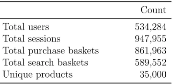
more than 90% of the purchases. After filtering, we cover about 947, 000 sessions made by ∼ 534, 000 users, which generated ∼ 861, 000 purchase baskets and ∼ 589, 000 search baskets consistings of products viewed. Observation counts from our working sample are presented in Table 1. In the paper, we use the terms viewed and searched interchangeably; both imply that the user opened the description page of the product.
Table 1: Observation counts from our working sample
Count
Total users 534,284
Total sessions 947,955
Total purchase baskets 861,963
Total search baskets 589,552
Unique products 35,000
Note 1: The table shows the size of our work-ing sample after filterwork-ing out purchases and searches involving right tail products. We re-tain the top-35,000 products that include more than 90% of the purchases in our sample pe-riod.
Note 2: Purchase baskets include products purchased and search baskets include products searched but not purchased. The number of searches baskets are less than the number of purchase baskets because we define a product searched only if the user opens the description page of the product. The user can, however, purchase without opening the product descrip-tion page by directly adding the product to the cart while browsing.
Product baskets: Purchases and searches
A typical user shopping session includes browsing a range of products, potentially across multiple categories, and then purchasing a subset of them. In this process, the user first forms a consideration set, i.e., a set of products from which the consumer intends to finally a choose from. In effect, from our model’s perspective, the user creates two product baskets during a shopping session — products viewed and products purchased, which form our units of analysis in this study. We distinguish between a purchased product basket and a searched product basket by including products that were purchased in the first one and viewed but not purchased in the second one respectively. In this paper, we refer to a purchased product basket simply as purchase basket and the searched product basket as search basket. For search baskets, we only include the product in the basket if the consumer opened its detailed
description page. It is important for us to distinguish between these two baskets since this separation allows us to learn different relationships between products, i.e., they could be potential complements or potential substitutes.
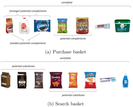
Figure1a shows an illustrative purchase basket. In this case, the user bought breakfast foods (coffee, milk, cookies), along with some snacks (chips and salsa), and two household products (toothpaste and dish pods). Our model and associated heuristics have been designed to infer that coffee, milk, and cookies are potential complements. Not only that, we want to go one step further and infer that coffee and milk are stronger complements than coffee and cookies. The signal for these relationships comes from thousands of purchase baskets where we are likely to find coffee and milk being purchased together more frequently than coffee and cookies. Similarly, we want to infer that chips and salsa are complements. The consumer in this case also purchased toothpaste and dish pods. Ex ante we do not expect any complementarity between these items and the rest of the basket and this may just be idiosyncratic noise particular to this shopping session. Note that the model does not make use of textual labels of the products. It ingests hashed product IDs and finds the relationships between these IDs, without ever looking at the product name or category.
We also observe the corresponding search basket of the same consumer, shown in Figure 1b. The search basket includes products that were viewed but not purchased together. We see that the consumer viewed different brands and flavors of coffee before purchasing one. Our model would infer them as potential substitutes. Further, the model would also pick out the different types of chips that the consumer searched. For inferring potential substitutes, we rely on the assumption that users search for multiple products before purchasing one, a pattern we do observe in the data.
Table 2 shows the summary statistics at a basket level. On average, a consumer searches 7 products for each one bought. The mean of products bought (or viewed) is higher than the median, indicating a long right tail of baskets with many products. Within each basket, the mean number of departments is 1.6, alluding to the concept of a focused shopping trip, i.e., a particular shopping session for groceries, a different one for household supplies, a third one for apparel, and so on. Further, we see that the average purchase basket consists of products from 3 different categories, i.e., a consumer like Esha described in the model section could be buying groceries for breakfast from different sub-categories such as coffee, milk, and cereal.
(a) Purchase basket
(b) Search basket
Figure 1: Illustrative purchase and search baskets created during a user shopping session
Table 2: Summary statistics per session
Purchased Viewed Products Mean 3.6 21.3 SD 4.2 34.1 Median 2 9 Max 202 1365 Department Mean 1.6 1.7 SD 0.8 1.0 Median 1 1 Max 10 14 Aisle Mean 2.4 2.6 SD 1.9 2.5 Median 2 2 Max 28 48 Category Mean 3.0 4.0 SD 2.9 5.3 Median 2 2 Max 69 122 Price Mean 44.6 303.7 SD 52.1 526.1 Median 32.3 127.4 Max 2,697 17,480
Note: A user session is defined a visit to the retailer’s website by a user. A session continues until there is no activity by the user for 30 minutes on the website. If the user performs an action after 30 minutes of inactivity, it is considered to be a new session by the same user.
5. Product embeddings
We train the model described in Section 3 using purchase and search baskets separately. Consequently, the model gives us two sets product embeddings (1) using purchase baskets that consist of product purchased together and (2) using search baskets by considering products that are viewed together but not purchased together.8 For training the models, we searched
for optimal hyper-parameters using a hold-out sample of the data. In the paper, we report results using the models trained with the optimally tuned hyper-parameters.
Purchase embeddings
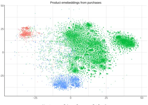
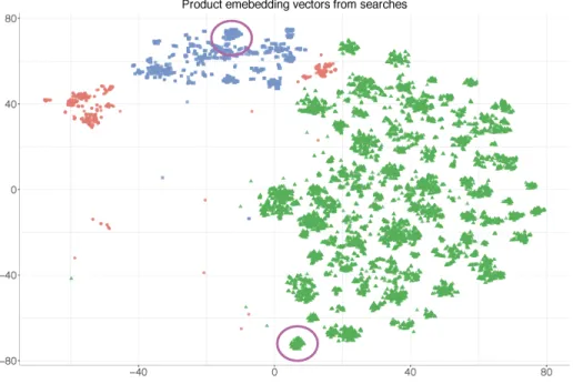
We generate purchase embeddings for products by extracting signals from their co-purchase history and condensing it to a 100-dimensional space. This is considerable gain in computa-tional efficiency as compared to a count-based model, where a unigram model would provide a binary representation in a 35, 000-dimensional space, equal to the number of products con-sidered. To get a perception of what the embeddings represent, we compress the embedding vectors to a 2-D space using t-SNE (van der Maaten and Hinton, 2008) and plot them in Figure2. For visual clarity, we highlight the department of the product and show products from three departments — groceries, baby, and pet products. A cursory glance reveals some obvious patterns. While we see a clear separation among products from different categories, there is also some overlap among departments. Again, in this space proximity to the other products indicates a higher likelihood of the two products occurring in similar contexts, or in our case, similar types of baskets. Proximity among the products in this space suggests a higher degree of complementarity9.
As a more granular example, we zoom into the grocery department and look at snack food, 8Given that our model relies solely on the co-occurrence of products within baskets, we only consider
baskets that have more than 1 product.
9These embeddings have been plotted in a latent space and hence the scale of this axis is immaterial and
−25 0 25 50
−25 0 25 50
H1category Baby Grocery Pet Supplies
Product emebeddings from purchases
Figure 2: Product embeddings using purchase baskets
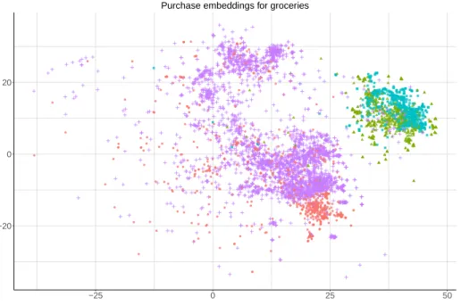
meats, dairy & eggs, and chocolates. Ex-ante we would be expect snack foods to have a stronger positive relationship with candy & chocolates, and meats to have a stronger relationship with dairy & eggs. Figure 3 presents evidence for this hypothesis with snack foods being much closer to candy & chocolates than to either meat products or dairy & egg products. In fact, there is considerable overlap among snack foods with candy & chocolates, suggesting a high degree of complementarity between them.
In addition to testing relationships among products from different but pre-existing categories (typically created by the retailer), we can also generate new sub-categories of products and check how well they go with products from other categories. For instance, in Figure 4, we compare organic groceries with snack foods. Although there is no pre-defined organic category of products, as a proof-of-concept, we do a simple string search of the word “organic” in the names of the products. We then visualize them along with snack foods to see what kind of organic products are related to snack foods. The upper highlighted portion of Figure 4 shows a high degree of complementarity among nuts, dried seeds such as watermelon seeds, trail mixes, jerky and dried meats, and seaweed snacks. On the other hand, the lower highlighted portion of the graph shown less of an overlap and mainly consists of cookies, chips & pretzels. We believe that having a flexible and scalable model such as ours can provide crucial insights about market structure, brand competition, product positioning, user
−20 0 20
−25 0 25 50
H2category Candy, Gum & ChocolateDairy & Eggs Meat & SeafoodSnack Foods
Purchase embeddings for groceries
Figure 3: Purchase embeddings for products within the grocery category
preferences, and personalized recommendations.
We dig deeper to the product level and, as examples, inspect a few focal products. Consider, for instance, organic potatoes. In the purchase space, the products closest to organic potatoes include other organic fruits and vegetables such as organic celery, organic grape tomatoes, and organic green bell peppers. Similarly, products closest to dish-washing liquid include other household items, and in some cases can be narrowed to the space of cleaning products, such as paper towels, laundry detergents, and steel cleaners. As a third example, we look at a product from the health and beauty category — Neutrogena Oil-Free Acne Wash Redness Soothing Cream Facial Cleanser. Products that go along with this facial cleanser and include other hygiene and beauty products such as liners, rash cream, body wash, and deodorant. More details about the close complements of these focal products along with their com-plementarity score (described later) are presented in the Appendix in TablesA.1,A.2, andA.3.
We take this visual and tabular evidence as support for our claim that products that frequently co-appear in product baskets tend to have a higher degree of complementarity between them.
Figure 4: Purchase embeddings for organic groceries and snack foods
Search embeddings
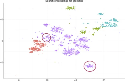
Similar to purchase embeddings, we generate product embeddings using historical co-views of products, i.e., by observing how frequently do products co-occur in consideration set formed during thousands of shopping trips. These embeddings also lie in a similar 100-dimensional space. We condense them to a 2-D space using t-SNE (van der Maaten and Hinton,2008) and plot them in Figure5. Again, we plot the same three departments — groceries, baby, and pet products. The overall theme of the embeddings remains largely similar to that in purchase embeddings. However, there are two notable distinctions. First, the inter-department clusters are further separated away indicating that most views are confined to within-department products. This reinforces the evidence we found in Table 2, where we found that most search sessions were confined to one department. Second, there are well-defined sub-clusters within the department cluster, which self-classify into finer aisles and categories. For instance, the lowest green cluster highlighted by the purple circle comprises only of “Breakfast Foods” (𝐴𝑖𝑠𝑙𝑒), primarily containing “Hot Cereals and Oats” (𝐶𝑎𝑡𝑒𝑔𝑜𝑟𝑦), with occasional presence of “Granola & Muesli” (𝐶𝑎𝑡𝑒𝑔𝑜𝑟𝑦). On the other end of the plot, the highlighted blue cluster on the top consists of supplies for our furry friends. This cluster only contains meat-based meals (𝐶𝑎𝑡𝑒𝑔𝑜𝑟𝑦) for dogs (𝐴𝑖𝑠𝑙𝑒). These observations also lend merit to our hypothesis that
Figure 5: Product embeddings using search baskets
At a more granular level, we look at aisles within the grocery department in Figure 6. We see more refined sub-clusters as compared to purchase embeddings for the same grocery products. For example, the highlighted cluster of purple points in the bottom of the graph is for popcorn and the highlighted cluster of purple points in the center left is for dried snack meats.
Similar to the purchase space, we inspect the same three products and calculate their prox-imity to other products in the search space. For example, organic potatoes are now closer to other varieties of potatoes in the search space such as golden potatoes, red potatoes, and even sweet potatoes, indicating a higher degree of substitutability among them. This in contrast to the purchase space where organic potatoes were closer to other organic fruits and vegetables. Similarly, dish-washing liquid is now closer to other types and brands of dish-washing detergents such as liquids and soaps of different scents and sizes. Finally, the acne face wash shows considerable similarity with varieties of acne face washes. However, in this case there is a strong brand effect with all potential substitutes being from the same brand - Neutrogena. It could be that users have strong preferences for brands when it comes to health and beauty products or that there is a single dominant brand in product line, another point we scrutinize in greater detail in a companion paper. More examples of products closer to each other in search space are provided in the Appendix in Tables A.4,A.5, and A.6.
Figure 6: Search embeddings for groceries
Product relationships
A critical ingredient in the recipe of our bundle generation process is the relationship between any two products in the retailer’s entire assortment. Furthermore, we want the relationship to be described by a metric that is continuous and category agnostic, so that we can compare the strengths of the relationships that a particular product has with other products in the assortment as well as compare strengths of the relationships across product pairs. In other words, we’d like to be able to make both within-product as well as between-product compar-isons. For example, we want to be able to say that coffee and cups are stronger complements than coffee and ketchup as well as that coffee and cups are stronger complements than tea and salt. This example seems obvious, however, it becomes increasingly hard to infer these relationships when there are thousands of products in the assortments and co-purchases among pairs of products are sparse. With 35,000 products in the retailer’s assortment, there are close to 50 million product combinations with over 90% of the co-purchases being zero. Moreover, we want these relationships to be inferred from the data we observe and not be pre-imposed by the retailer. Analogously, we want to be learn that coffee and tea are stronger substitutes than coffee and fruit juice.
With this objective in mind and based on the evidence described above, we generate a heuristic for the degree of complementarity between products 𝑖 and 𝑗 in the purchase space,
𝐶𝑖𝑗 ,
𝑢𝑏 𝑖 · 𝑢𝑏𝑗
‖𝑢𝑏‖‖𝑢𝑏‖, (7)
where 𝑢𝑏𝑖 and 𝑢𝑏𝑗 are the embeddings of products 𝑖 and 𝑗 in the purchase space respectively, and ‖ · ‖ is the norm of the embedding vector. This heuristic is similar to the one used by Ruiz et al. (2017).
Similarly, we generate a heuristic for the degree of substitutability between two products 𝑖 and 𝑗 in the search space,
𝑆𝑖𝑗 ,
𝑢𝑠 𝑖 · 𝑢𝑠𝑗
‖𝑢𝑠‖‖𝑢𝑠‖, (8)
where 𝑢𝑠𝑖 and 𝑢𝑠𝑗 are the embeddings of products 𝑖 and 𝑗 in the search space respectively, and ‖ · ‖ is the norm of the embedding vector.
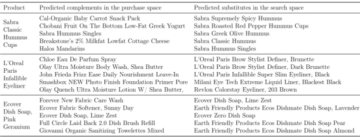
To give an overview of what these product relationships look like, we present examples with a few focal products. For instance, in Table 3, we show the top-5 complements of products from three categories. In the first section, we consider hummus and we see that strong complements with it are baby carrots, greek yogurt and mandarins. On the other hand, substitutes are other varieties of hummus. Similarly, for eyeliner, we find that complementary products include other skin-care and beauty products, whereas its substitutes are other varieties of eyeliner. Lastly, for household cleaning products such as dish soap, we find other types of cleaning products as strong complements, and other varieties of dish soap as strong substitutes.
Table 3: Product relationships using the complementarity and substitutability heuristic
Product Predicted complements in the purchase space Predicted substitutes in the search space Sabra
Classic Hummus Cups
Cal-Organic Baby Carrot Snack Pack Sabra Supremely Spicy Hummus
Chobani Fruit On The Bottom Low-Fat Greek Yogurt Sabra Roasted Red Pepper Hummus Cups
Sabra Hummus Singles Sabra Greek Olive Hummus
Breakstone’s 2% Milkfat Lowfat Cottage Cheese Sabra Classic Hummus
Halos Mandarins Sabra Hummus Singles
L’Oreal Paris Infallible Eyeliner
Chloe Eau De Parfum Spray L’Oreal Paris Brow Stylist Definer, Brunette
Olay Ultra Moisture Body Wash, Shea Butter L’Oreal Paris Brow Stylist Definer, Dark Brunette John Frieda Frizz Ease Daily Nourishment Leave-In L’Oreal Paris Infallible Super Slim Eyeliner, Black Smashbox NEW Photo Finish Foundation Primer Pore Milani Eye Tech Extreme Liquid Liner, Blackest Black Olay Quench Ultra Moisture Lotion W/ Shea Butter, Revlon Colorstay Eyeliner, 203 Brown
Ecover Dish Soap, Pink Geranium
Forever New Fabric Care Wash Ecover Dish Soap, Lime Zest
Ecover Fabric Softener, Sunny Day Earth Friendly Products Ecos Dishmate Dish Soap, Lavender
Ecover Dish Soap, Lime Zest Ecover Zero Dish Soap
Full Circle Laid Back 2.0 Dish Brush Refill Earth Friendly Products Ecos Dishmate Dish Soap Pear Giovanni Organic Sanitizing Towelettes Mixed Earth Friendly Products Ecos Dishmate Dish Soap Almond
Note: For each focal product, the table shows the top-5 complements as determined by the embeddings in the purchase space and the top-5 substitutes as determined by the embeddings in the search space.
6. Bundle generation and field
experiment
We follow a two-stage strategy to design bundles. In the first stage, we create a candidate set of bundles using the metrics of complementarity and substitutability described above and run a field experiment to gauge consumer preferences for different types of bundles. The motivation here is to develop a principled exploratory strategy that is based on a more refined action space derived using historical purchases and consideration sets. Following the field ex-periment, we move to the second stage in which we model the association between the product relationship heuristics and bundle preferences, verify the robustness of the association, and generate better bundles based on these metrics as well as certain pre-experiment co-variates. The “learning” happens in this stage from the mapping of metrics and the co-variates to the purchase rates of the bundles. This allows us to scale our bundle generation process to the entire assortment of products, enabling retailers to identify good candidates for bundles that consumers would prefer, thereby generating additional value for their customers.
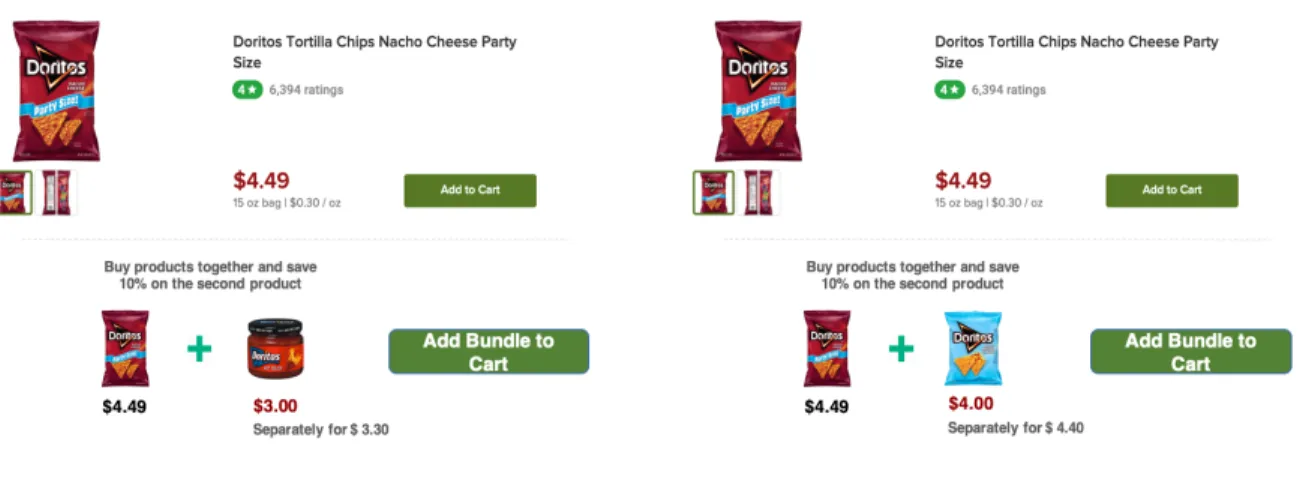
We describe our strategy to create a candidate set of bundles for the field experiment below. In what follows, we consider bundles of two products — a “focal” product and an “add-on” product. The focal product is the main product on whose page the bundle offer is shown and the add-on is the product on which the discount is applied. An illustrative example of how this is implemented on the retailer’s website is shown in the Figure 7. In order to facilitate a direct comparison between the different bundles, we offer the same relative discount on all the bundles — 10% off on the add-on product and full price for the focal product. The discount percentage was selected after discussions with the retailer. Before we explain the different bundle types, it is worth mentioning that the idea behind the experiment is not to horse-race different bundle types but rather learn a good strategy of making bundles as a function of the scores. By selecting bundles from different categories and departments, we intentionally add variation to explore a wider range of bundles, albeit in a principled way.
(a) Complementary bundle example (b) Variety bundle example
Figure 7: Illustrative example from the field experiment
Candidate bundles
Our primary motivation here it to explore the potential space of bundles to generate a candidate set whose performance will be empirically validated using a field experiment. To this end, we leverage the relationships identified between products and generate a varied set of bundles. Specifically, for each focal product, we create multiple bundles across different categories, casting a wide exploratory net for learning consumer preferences, while exploiting the strength of relationships between products to guide the learning. For the field experiment, we create four types of bundles for 4, 500 products as follows:
1. Co-purchase bundles (CP): The first category of bundles is based on high observed co-purchase frequency. For each focal product, we select the product that it has been most frequently co-purchased with. These bundles are the natural contenders for a simple data-driven bundling strategy - products that have been purchased frequently together in the past will have a higher likelihood of being purchased together in the future as well, ceteris paribus. They also serve as a useful starting point of our bundle design strategy since we can map these bundles back to the underlying complementarity and substitutability scores, allowing us to learn more generalized patterns. However, these bundles are limited in scope since this strategy (a) does not generate bundles of products that have never been co-purchased before, (b) uses co-purchase information even when it is very noisy, e.g., bundling products if they have been co-purchased, say, 2 times in the past, (c) does not explore cross-category options since most of the bundles come from the same categories and aisles. An example of this type of bundle is
toothpaste and toothbrush.
2. Cross-category complements (CC): For a focal product 𝑖, we consider the strongest complement for 𝑖 across a different category but within the same department. The idea behind this strategy is to identify products that are most likely to be complements in usage and hence having the focal product under consideration would indicate a high-likelihood of purchasing the add-on product as well. However, to add an element of exploration, we pair products across different categories. In case of a tie with the above co-purchase bundles, we use the second strongest complement. A simple example of this is bundling toothpaste and mouthwash.
3. Cross-department complements (DC): These bundles are similar in spirit to the cross-category complementary bundles mentioned above except that they specifically search over departments that are different from that of the focal product. Since most purchases within a trip come from the same department, as shown in Table2, we tend to find stronger complements within the same department. Hence, the motivation in this arm is to explore cross-department bundles (e.g., household supplies and beauty products) of products that would otherwise not be considered. An example for this would be bundling toothpaste and night cream together.
4. Variety (VR): Extant research has suggested the benefit of bundling (imperfect) substitutes to capture a larger portion of the consumer surplus and improve profitability (Lewbel, 1985; Venkatesh and Kamakura, 2003). We explore this idea empirically by creating bundles of products that are close to each other in the search space. The rationale here is that products that appear to be potential substitutes may in fact also be complements over time or complements within a household. If this is true, then bundling products that are imperfect substitutes could help exploit variety seeking behavior among consumers and generate incremental sales for the retailer. For example, bundling two different varieties or flavors of toothpaste.10
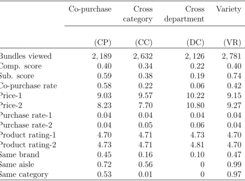
We create 18, 000 bundles across the different types mentioned above. Basic characteristics of the bundles across the four types are shown in Table 4. We show the results for 9, 728 bundles which were viewed at least once during the experiment, and hence are part of our subsequent analysis. All values in this table are calculated based on the pre-experiment data used for training. The number of bundles viewed is different across the four bundle 10There is obviously the caveat that consumers may actually be forward looking and just buy the products
ahead of time while they are being sold at a discount thereby having no impact on overall sales of the retailer. We do not investigate inter-temporal substitution patterns in this study while noting that it is a interesting avenue to study further.
types since there is flux in the inventory and depending upon the location and time of the consumer, a bundle may or may not be available. We also provide a similar table us-ing focal products that have all the different bundle types viewed in TableA.7in the Appendix.
We calculate the co-purchase rate for the product pairs. Price-1, Rating-1, Purchase rate-1 correspond to the average price of the focal products, their average user provided ratings, and their historical individual purchase rates. Analogously, Price-2, Rating-2, and Purchase rate-2 correspond to the same variables for the add-on product. The last three rows show the mean of binary variables which take the value 1 if both the product belong to the same brand, same aisle, and the same category respectively.
Table 4: Bundle types based on relationship heuristics
Co-purchase Cross Cross Variety
category department (CP) (CC) (DC) (VR) Bundles viewed 2, 189 2, 632 2, 126 2, 781 Comp. score 0.40 0.34 0.22 0.40 Sub. score 0.59 0.38 0.19 0.74 Co-purchase rate 0.58 0.22 0.06 0.42 Price-1 9.03 9.57 10.22 9.15 Price-2 8.23 7.70 10.80 9.27 Purchase rate-1 0.04 0.04 0.04 0.04 Purchase rate-2 0.04 0.05 0.06 0.04 Product rating-1 4.70 4.71 4.73 4.70 Product rating-2 4.73 4.71 4.81 4.70 Same brand 0.45 0.16 0.10 0.47 Same aisle 0.72 0.56 0 0.99 Same category 0.53 0.01 0 0.97
Note 1: Co-purchase rate has been multiplied by 100. Price-1, Purchase rate-1, and Product rating-1 show the average price, average historical purchase rate, and the average product rating of the focal product in each bundle type. Price-2, Purchase rate-2, and Product rating-2 are corresponding variables for the add-on product. Same brand, Same aisle, and Same category are binary variables that indicate if the two products are from the same brand, same aisle, and the same category respectively.
Note 2: For 26 bundles in the CC type, the add-on product category had been incorrectly recorded in the retailer’s database. We note their correct category here and all subsequent analysis is done with the correct category.
Finally, we note that our focus here is on identifying the best promotional bundles for consumers and we do not explicitly optimize for profitability or revenue maximization, which
in itself is a challenging computational pursuit. However, we do put reasonable constraints on the bundles we create after deliberations with the retailer. Specifically, we only create bundles containing products with net positive margin after including the 10% discount.
Field experiment
Our algorithm to create product embeddings and learn product relationships allows us to generate a wide set of candidate bundles that consumers would prefer. Our goals with the field experiment are to empirically validate how different bundles perform and learn high-level strategies that can be effectively implemented by managers.
We ran the field experiment for two months from mid-July 2018 to mid-September 2018. The experiment was run at a user-product level, such that if a user 𝑚1 searched for product 𝑖
which has a bundle associated with it, then the user would be randomized into one of the four treatments, i.e., the consumer would be shown one of the four bundles associated with the focal product. Let’s say that user 𝑚1 was randomized into the cross-category complement
bundle arm for product 𝑖, then every time 𝑚1 searched for 𝑖, she would be offered the
opportunity to buy the cross-category complement bundle with the discount. The user need not buy the bundle and can still purchase either the focal product directly or the add-on product without any discount. After searching for 𝑖, if 𝑚1 searched for product 𝑗, she would
again be randomized into any of the four treatments. However, if she searched for 𝑖 again, she would be in the same cross-category complement treatment. To give a perspective of how the bundle offer is presented to the user, we show two illustrative examples in Figure 7.
As expected due to the randomization, pre-experiment covariates — number of visits, number of product views, number of different products added-to-cart, total number of units purchased (accounting for multiple units of the same product purchased), and total revenue — are
statistically indistinguishable across the different bundle types (Appendix, Table A.8).
An overview of the results from the field experiment is shown in Table 5. 9, 728 bundles were viewed a total of 356, 368 times by 164, 469 users during the experiment. A visit to a bundle is the same as the visit to the focal product (as shown in Figure7). We also capture clicks on the bundle component on the web page, the number of bundles added-to-cart (ATC), and bundle purchases. The third column shows the same metrics as a proportion of the total number of bundle views.
Table 5: Key metrics from the field experiment
Count Count/
Views
Unique bundles viewed 9, 728
-Total bundle views 356, 368
-Bundle clicks 5, 197 0.015
Bundle ATC 2, 847 0.008
Bundle purchases 503 0.001
Note: The third column is the second column divided by the total number of views. ATC is add-to-cart.
We further investigate the results split by bundle type. Table 6shows variation in the views, clicks, and purchases of bundles across the different bundle types. We focus on two metrics of success for the bundles — the add-to-cart rate and the purchase rate. Add-to-cart (ATC) rate is the ratio of add-to-cart events and total views and the purchase rate is the ratio of bundle purchases to total views. These rates are largely highly statistically significantly different between pairs of types (Table A.9 in the Appendix).
To reiterate, the aim here was to try a refined sampling of bundles so as to explore the action space and learn bundle success likelihood as a function of the underlying scores. Consequently, we don’t dive too deep into the comparative results of the experimental bundle types. However, we do note a few interesting points. First, as is expected, the co-purchase bundles (CP), consisting of products that have been frequently purchased together in the past, tend to do quite well. Adding a discount to frequently co-purchased bundles would have further increased their likelihood of purchase. However, as mentioned earlier, most of these bundles come from the same aisle and do not exploit the range of the retailer’s assortment. The embeddings allows us to tap into that variation systematically by mapping these bundles to the under-lying product relationship scores. We describe this process in greater detail in the next section.
Variety bundles (VR) have a high purchase rate as well and their performance is similar to co-purchase bundles (CP). The cross-category complements (CC) have a lower purchase rate as compared to co-purchase and variety bundles. Further, while the cross-department (DC) bundles did not perform as well as the other categories but they provide interesting insights into cross-department promotion strategies. For example, a popular cross-department bundle was between household supplies and skin care — laundry detergent + hand soap. Other
popular cross-department bundles include coffee + paper napkins, and shower cleaner + whitening toothpaste. Correspondingly, popular cross-category bundles were granola bars + crackers, mops + floor cleaners, and disposable razors + body wash. Popular variety bundles mostly consisted of close, but still imperfect, substitutes such as frozen meals with vegetable korma + Bombay potatoes, snacks such as organic pumpkin seeds + organic raw almonds, and pasta with gluten free rotini + gluten free penne. In fact, grocery variety bundles performed particularly well.
Table 6: Experiment results split by bundle type
Co-purchase Cross-cat. Cross-dept. Variety
(CP) (CC) (DC) (VR) Bundles 2, 189 2, 632 2, 126 2, 781 Views 94, 458 88, 757 81, 239 91, 914 Clicks 1, 586 1, 014 794 1, 803 ATC 1, 050 665 289 843 Purchases 198 102 47 156 CTR 0.017 0.011 0.010 0.020 ATC rate 0.011 0.008 0.004 0.009 Purchase rate 0.002 0.001 0.001 0.002
Note 1: CTR is click-through rate. ATC is add-to-cart. The rate columns in the right half of the table are calculated as a proportion of views.
The field experiment serves an intermediate step that bring us closer to the focal task ideniti-fying good bundles from the entire assortment. By systematically adding variation across different bundle types we are able to learn consumer preferences across a range of bundles coming from multiple categories of the retailer’s assortment. However, by themselves, individ-ual bundle results are quite noisy and do not directly lend themselves towards implementable insights. In the next section we tie the relationship scores from the embeddings with the results from the experiment using predictive modeling to derive more general and robust findings.
7. Generalization with supervised
learning
Results from the field experiment show that there is value in using the underlying product embeddings to generate product bundles. This is coarsely illustrated in Figure 8, which shows the performance of the bundles across quintiles of the two relationship heuristics. While this suggests that the heuristics are a good approach to form promotional bundles, it also is a fertile exploratory ground to identify more, and perhaps even better, bundles. To systematically explore the space of bundles, we build a supervised learning model to harness the value in the product relationships and predict bundle success likelihood.
0.000 0.005 0.010 0.015
1 2 3 4 5
Comp. score quintile
Bundle add−to−car
t r
ate
(a) Complementarity score
0.000 0.005 0.010
1 2 3 4 5
Sub. score quintile
Bundle add−to−car
t r
ate
(b) Substitutability score
Figure 8: Bundle add-to-cart rate as a function of relationship scores
We do this using a hierarchical logistic regression, allowing the intercept and slopes for the product relationship variables to vary at the aisle level, as shown in Equation10.