Routine uncertainty propagation for the marine carbon dioxide system

HAL Id: hal-01973728

https://hal.sorbonne-universite.fr/hal-01973728

Submitted on 8 Jan 2019

HAL is a multi-disciplinary open access

archive for the deposit and dissemination of

sci-entific research documents, whether they are

pub-lished or not. The documents may come from

teaching and research institutions in France or

abroad, or from public or private research centers.

L’archive ouverte pluridisciplinaire HAL, est

destinée au dépôt et à la diffusion de documents

scientifiques de niveau recherche, publiés ou non,

émanant des établissements d’enseignement et de

recherche français ou étrangers, des laboratoires

publics ou privés.

Distributed under a Creative Commons Attribution| 4.0 International License

dioxide system

James C. Orr, Jean-Marie Epitalon, Andrew Dickson, Jean-Pierre Gattuso

To cite this version:

James C. Orr, Jean-Marie Epitalon, Andrew Dickson, Jean-Pierre Gattuso. Routine uncertainty

propagation for the marine carbon dioxide system. Marine Chemistry, Elsevier, 2018, 207, pp.84-107.

�10.1016/j.marchem.2018.10.006�. �hal-01973728�

Contents lists available atScienceDirect

Marine Chemistry

journal homepage:www.elsevier.com/locate/marchem

Routine uncertainty propagation for the marine carbon dioxide system

James C. Orr

a,⁎

_{, Jean-Marie Epitalon}

b

_{, Andrew G. Dickson}

c

_{, Jean-Pierre Gattuso}

d,e

a_{Laboratoire des Sciences du Climat et de l'Environnement, LSCE/IPSL, CEA-CNRS-UVSQ, Université Paris-Saclay, Gif-sur-Yvette, France} b_{Geoscientific Programming Services, Fanjeaux, France}

c_{University of California, San Diego (UCSD), La Jolla, CA, USA}

d_{Sorbonne Université, CNRS, Laboratoire d'Océanographie de Villefranche, Villefranche-sur-mer, France} e_{Institute for Sustainable Development and International Relations, Sciences Po, Paris, France}

A R T I C L E I N F O Keywords: Carbonate chemistry Uncertainty propagation Carbon dioxide pH Alkalinity

Dissolved inorganic carbon Ocean acidification

A B S T R A C T

Pairs of marine carbonate system variables are often used to calculate others, but those results are seldom reported with estimates of uncertainties. Although the procedure to propagate these uncertainties is well known, it has not been offered in public packages that compute marine carbonate chemistry, fundamental tools that are relied on by the community. To remedy this shortcoming, four of these packages were expanded to calculate sensitivities of computed variables with respect to each input variable and to use those sensitivities along with user-specified estimates of input uncertainties (standard uncertainties) to propagate uncertainties of calculated variables (combined standard uncertainties). Sensitivities from these packages agree with one another and with analytical solutions to within 0.01%; similar agreement among packages was found for the combined standard uncertainties. One package was used to quantify how propagated uncertainties vary among computed variables, seawater conditions, and the chosen pair of carbonate system variables that is used as input. The relative contributions to propagated uncertainties from the standard uncertainties of the input pair of measurements and various other input data (equilibrium constants etc) were explored with a new type of diagram. These error-space diagrams illustrate that further improvement beyond today's state-of-the-art measurement uncertainties for the input pair would generally be ineffective at reducing the combined standard uncertainties because the contribution from the constants is larger. Likewise, using much more uncertain measurements of the input pair does not always substantially worsen combined standard uncertainty. The constants that contribute most to combined standard uncertainties are generally K1and K2, as expected. Yet more of the propagated uncertainty in the computed saturation states of aragonite and calcite comes from their solubility products. Thus percent re-lative combined standard uncertainties for the saturation states are larger than for the carbonate ion con-centration. Routine propagation of these uncertainties should become standard practice.

1. Introduction

Scientists commonly constrain the marine carbonate system by mea-suring two of its variables and using that pair to calculate the others. Less common is to report the propagated uncertainties of the calculated vari-ables. Although the approach to propagate those uncertainties is well es-tablished (Dickson and Riley, 1978), it must be implemented by scientists, individually, because it is not an option in related public software packages (Orr et al., 2015). This technical gap may explain why these uncertainties are not routinely reported, even for efforts such as the ocean acidification community's long-term data compilation initiative (Nisumaa et al., 2010; Yang et al., 2016).

Among the limited studies that have reported propagated uncertainties, approaches and assumptions differ. Most have used Gaussian uncertainty

propagation (Dickson and Riley, 1978; Millero, 1995, 2007;McLaughlin et al., 2015;Sutton et al., 2016); others have used a Monte Carlo approach (Fassbender et al., 2016a;Williams et al., 2017) or a simpler but related method. That simpler approach was taken byLauvset and Gruber (2014) who suggested that the Gaussian approach underestimates propagated un-certainties when its linear approximations (first order Taylor series) are applied to solve the series of nonlinear equations inherent in the marine CO2

system. That concern, if generally true, would undermine previous work. Yet the approach is not the only source of differences between studies. Studies that have used the Gaussian approach have considered uncertainties both in the measured input pair of carbonate system variables and in the equilibrium constants needed to make these calculations; conversely, with the full or simplified Monte Carlo approach, onlyWilliams et al. (2017) have accounted for uncertainties from the equilibrium constants.

https://doi.org/10.1016/j.marchem.2018.10.006

Received 15 June 2018; Received in revised form 14 October 2018; Accepted 16 October 2018 ⁎_{Corresponding author.}

E-mail address:james.orr@lsce.ipsl.fr(J.C. Orr).

Available online 26 October 2018

0304-4203/ © 2018 The Authors. Published by Elsevier B.V. This is an open access article under the CC BY-NC-ND license (http://creativecommons.org/licenses/BY-NC-ND/4.0/).

But to what extent do uncertainties in the equilibrium constants matter? Dickson and Riley (1978) found that these uncertainties were usually a minor contributor to the overall propagated uncertainty, unlike un-certainties in the input pair of carbonate system variables. But decades have elapsed, and measurement accuracy and precision have improved.Millero (1995)used lower uncertainty estimates for both input variables and con-stants, finding that contributions from the constants to the overall propa-gated uncertainty were no longer a minor contributor although they were generally outweighed by the contribution from the input pair of measure-ments. Dickson (2010)reevaluated propagated uncertainties, using three sets of estimates for measurement uncertainties, while maintaining the same set of uncertainty estimates for the dissociation constants and using the same sensitivities fromDickson and Riley (1978)(Table 1). In that update, uncertainties from the constants generally dominated the overall propa-gated uncertainty when present-day, state-of-the-art methods were used with reference materials; conversely, with other methods, uncertainties in measurements of the input pair contributed most to the overall propagated uncertainty. Yet propagated uncertainties will differ with choices for input uncertainties, with geographic variations in input variables, and with con-sequent changes to the sensitivities of computed variables to input variables. The original sensitivities fromDickson and Riley (1978)remain in use today (e.g.,Dickson, 2010;Sutton et al., 2016). However those were provided for only one particular set of seawater conditions (temperature T = 25C, sali-nity S = 35, carbonate alkalisali-nity AC= 2248 μmol kg−1, total dissolved

inorganic carbon CT= 2017 μmol kg−1, and zero nutrients). Much less of a

concern is that the first and second dissociation constants of carbonic acid, K1and K2, used byDickson and Riley (1978)have changed. When those are

converted from the NBS to the total scale, they agree within about 1% (at 25C) of the values now recommended for best practices (Lueker et al., 2000). The most important factor for uncertainty propagation of the marine CO2system is the choice of input uncertainties themselves, particularly for

the dissociation constants. Choices of standard uncertainties for pK1and pK2

(u(pK1) and u(pK2)) have ranged from 0.2 to 0.75 times the values used by Dickson and Riley (1978)(Table 1). Thus the proposed uncertainties in K1

and K2(u(K1) and u(K2)) have also ranged from about 20 to 75% of the

Dickson and Riley (1978) values because for small uncertainties u(Ki)/ Ki= 2.3 u(pKi).

In recent years, uncertainties of carbonate system variables have been discussed in the context of establishing a Global Ocean Acidification Observing Network (GOA-ON) (Newton et al., 2015). To ensure that mea-surements are of appropriate quality to address the relevant problems, GOA-ON has proposed two levels of uncertainty. The GOA-GOA-ON Weather goal is aimed at assessing spatial and short-term variations (e.g., diurnal varia-bility), while its Climate goal is stricter, focusing on deciphering decadal trends. To frame its Weather goal, GOA-ON has proposed that the relative uncertainty in calculated carbonate ion concentration [CO32−] must

be < 10%, while for the Climate goal, the uncertainty for a difference in [CO32−] over time must be < 1%. While the Weather goal focuses on

in-dividual measurements, the Climate goal emphasizes the need to identify trends. These thresholds have been used to back calculate the corresponding maximum permissible uncertainties in measured input variables. For the Weather goal, GOA-ON estimates that measurement uncertainties must be no larger than 0.02 for pH, 10 μmol kg−1_{for total alkalinity A}

Tand

dis-solved inorganic carbon CT, while pCO2must have a relative uncertainty of

no more than 2.5%. For the Climate goal, corresponding estimates are 0.003 for pH, 2 μmol kg−1_{for A}

Tand CT, and 0.5% for pCO2. A recent

inter-laboratory comparison suggests that most research groups currently mea-suring ocean pH, AT, and CTare able to make those measurements within

the criteria of the Weather goal, whereas rather few were able to achieve the Climate goal (Bockmon and Dickson, 2015). The same study hints that many groups may underestimate the true uncertainty in their measurements. Falling into this category would be research groups whose uncertainty es-timates are based only on repeatability (short-term precision), i.e., not considering other possible sources of uncertainty (De Bièvre, 2008).

Traditionally, uncertainty propagation has involved identifying sources of bias (systematic errors), correcting for those as best as possible, and then propagating remaining random uncertainties (Taylor, 1996). But that changed when the International Organization for Standardization (ISO) published the Guide to the Expression of Uncertainty in Measurement (GUM, 1993), followed two years later by Eurachem's guide, subsequently

Table 1

Various estimates of standard uncertainties in input variables and constants.

Variablea _{Previous work This study Units}

DR78b _M95b _M06b _M07b _D10ac _D10bc _D10cc _McL15d _{Random Total}

AT 9, 2 4 3 3 1.2 2–3 4–10 5 2 2 μmol kg−1 CT 10, 4 2 2 2 1 2–3 4–10 5 2 2 μmol kg−1 pCO2 7 2 2 2 1 2 5–10 6 2 2 μatm pH 0.01 0.002 0.002 0.002 0.003 0.005 0.01–0.03 0.01 0.003 0.01 pK0 0.002 0.002 0.002 0.002 0.002 0.002 0.002 pK1 0.01 0.002 0.006 0.002 0.01 0.01 0.01 0.0075 0.0055e 0.0075 pK2 0.02 0.005 0.011 0.005 0.02 0.02 0.02 0.015 0.01e 0.015 pKB 0.01 0.01 pKW 0.01 0.01 pKA 0.02f 0.02 pKc 0.02f 0.02 BT/S 0.02g

a _{These variables are defined as in chapter 2 ofDickson et al. (2007)except that here we write pCO}

2rather than p(CO2). The equilibrium constants K0, K1, K2, KB etc. are in their conventional logarithmic form: pK = −log10K, while S is practical salinity. Thus whenever we refer to [H+] we mean the amount content (mol kg−1_{) of “total hydrogen ion” (i.e., implicitly accounting for interactions with sulfate). Thus here as inDickson et al. (2007), pH is defined as −log}

10[H+] rather than the more conventional log10(a[H+]) (Buck et al., 2002). This definition ensures compatibility with the recommended (Dickson et al., 2007) stoichiometric acid dissociation constants for seawater media.

b _{Input fromDickson and Riley (1978),Millero (1995),Millero et al. (2006), andMillero (2007), respectively. M06 also estimated u(pK}

1) and u(pK2) for earlier formulations. Numbers from DR78 and M07 are based on precision, not accuracy.

c _{Input fromDickson (2010), Table 1.4 for (a) reference methods, (b) state-of-the-art, and (c) other.} d_{Input fromMcLaughlin et al. (2015)}

e _{Based on the sample standard deviation of the difference between observed and predicted values for theMehrbach et al. (1973)constants refitted byLueker et al.}

(2000).

f _{Based on a 5% relative uncertainty (precision) fromMucci (1983)} g _{Relative uncertainty (equivalent to 2%)}

updated (Ellison and Williams, 2012), that emphasized GUM's application to analytical chemistry. GUM emphasized that the overall uncertainty in-cludes all sources of uncertainty, both random and systematic, that both those kinds of uncertainties should be expressed as standard deviations, and that systematic as well as random uncertainties should be propagated to-gether. GUM further clarified that if its sign and magnitude are known, the systematic error should be removed before propagating uncertainties while noting that such correction is imperfect and leaves a residual bias that should itself be treated as an uncertainty contribution; otherwise systematic uncertainty should be treated in the same way as random uncertainty, whether it was determined statistically (Type A) or by other means (Type B), such as by comparison to reference materials or by professional judg-ment. Although revolutionary at the time, the GUM principles have been widely adopted by the community, particularly by metrology institutes such as the National Institute of Standards and Technology (NIST).

Following suit, we adopt GUM's technical terminology and approach. For example, error and uncertainty are not synonyms. The error is the difference between a measured value and the true value. Since the true value cannot be known, neither can the error. The error may be positive or negative, while the uncertainty is always non-negative. That is, the un-certainty is the half-width of the interval around a measured value that is expected to contain the true value given a certain probability. The un-certainty of a measurement when characterized by its standard deviation is denoted as the standard uncertainty u. When the standard uncertainties of the input variables are used to propagate the uncertainty of a calculated variable, as outlined in GUM, the result is referred to as the combined standard uncertainty uc. Often, ucis multiplied by a coverage factor k to

obtain the expanded uncertainty U, the half-width of a confidence interval that is expected to include the true value. For example, with k = 1, 2, or 3, there is 68, 95, or 99.7% confidence that the true value falls within the ± kuc interval centered around the calculated value, assuming the

variable is normally distributed.

Given the basic scientific requirement to understand uncertainty, ex-perts from the ocean acidification community have emphasized the need to enhance existing CO2 system software packages to allow them to also

propagate uncertainties (Martz et al., 2015). Here our main aim is to do just that, thus providing marine scientists with public tools to easily propagate uncertainties using (1) automatically calculated sensitivities, which vary from region to region, and (2) input standard uncertainties that may be user specified. Standard uncertainties should be estimates that include both random and systematic components. Standard uncertainties based only on repeatability of measurements (precision) will underestimate the overall propagated uncertainty. Input uncertainties should be given as standard uncertainties u, as adopted here, so that computed outputs are the combined standard uncertainties uc. In addition, we aim to quantify the contributions

to the combined standard uncertainties calculated by the enhanced software packages and offer the ability to assess the extent to which they are affected by using alternative measurement techniques with lower or higher standard uncertainties.

2. Methods

Below we detail the approaches taken to compute sensitivities and propagate uncertainties, explain our choice of two sets of input un-certainties, and illustrate how results from the new routines can be syn-thesized graphically to provide a wider perspective.

2.1. Approaches

The classic way to propagate uncertainties is to use a first-order Taylor series expansion. For example, for an equation with two independent variables, y = f(x1,x2), the combined standard uncertainty in the dependent

variable y is = + + u y y x u x y x u x y x y x u x x ( ) ( ) ( ) 2 ( , ) c2 1 2 2 1 2 2 2 2 1 2 1 2 (1)

where squared uncertainties are treated as a variances, i.e., uc2(y) is the

squared combined standard uncertainty for y, u2_(x

1) is the squared standard

uncertainty for x1, and u2(x2) is that for x2, while the terms in parentheses

on the right-hand side are the sensitivities of the dependent variable to each independent variable and u(x1,x2) is the covariance between the standard

uncertainties in x1and x2. The covariance is the product of the individual

standard uncertainties and the correlation coefficient, namely u(x1,x2) = u

(x1) u(x2) r(x1,x2) where −1 ≤ r(x1,x2) ≤ 1. Many are familiar with Eq.(1)

only when the final covariance term is neglected, a simplification that is justified when x1and x2are uncorrelated; sometimes though, that is a poor

assumption (Taylor, 1996;Tellinghuisen, 2001). Generalizing for n depen-dent variables, the propagation-of-uncertainties equation becomes

= = = u y y x y x u x x ( ) ( , ) c i n j n i j i j 2 1 1 (2)

which follows the classical form of Eq.(1)given that the covariance of a variable with itself is its variance u(xi,xi) = u2(xi) and that covariances are

also symmetric, i.e., u(xi,xj) = u(xj,xi).Dickson and Riley (1978)applied the

classic approach of propagation of uncertainties to the ocean carbonate system while neglecting covariances and expressing the equation in terms of relative uncertainties. That is, they neglected terms in Eq.(2)where i ≠ j, divided both sides of that by y2_{, and multiplied the right side by (x}

i/xi)2to come up with = = u y y y y x x u x x ( ) / / ( ) _, c i n i i i i 2 1 2 2 (3) The left-hand side is the square of the relative combined standard un-certainty in y, a function of the right-hand side's squared relative standard uncertainties of each input variable (u(xi)/xi), multiplied by the square of

the associated relative sensitivity term (∂y/y)/(∂xi/xi), which is the same as

(∂ ln (y))/(∂ ln (xi)). Thus it is simple to understand the percent relative

combined standard uncertainty in y as a function of a 1% relative standard uncertainty in each xi, neglecting other contributions. The general approach

shown in Eq.(2)may also be expressed in matrix form (Appendix A). Eq.(2)is the most common form of the Method of Moments because it uses a first-order approximation of y to estimate that dependent variable's second moment, i.e., its standard deviation uc(y); when covariance terms are

neglected, it simplifies to the Gaussian approach (Taylor, 1996;Kirchner, 2001). We implemented both approaches in four public software packages that are commonly used to compute marine carbonate chemistry: CO2SYS-Excel (Pierrot et al., 2006), CO2SYS-MATLAB (van Heuven et al., 2011), mocsy (Orr and Epitalon, 2015), and seacarb (Proye and Gattuso, 2003; Lavigne and Gattuso, 2011; Gattuso et al., 2018). In the current im-plementation, users may specify the covariance between the uncertainties of the input pair of carbonate system variables. Other covariances are assumed to be negligible. Users may also exploit the intermediate routines that compute the absolute sensitivities (partial derivatives) needed for un-certainty propagation. These sensitivities of output variables to input vari-ables, also known as buffer factors (Frankignoulle, 1994), are useful by themselves to assess rates of change and help deconvolve responsible me-chanisms using Taylor series. A third approach was included in one public package for comparison. Rather than calculating sensitivities, the Monte Carlo approach relies on random number generation. That is, it computes the uncertainty in the output variable as the standard deviation of results from many calculations, each of which randomly selects each input variable from an assumed probability distribution, typically Gaussian, characterized by its input value and uncertainty (mean and standard deviation). Con-versely, the Gaussian and Method of Moments approaches are valid in-dependent of the probability distribution, which is often unknown. 2.2. Sensitivities

To propagate uncertainties with both the Gaussian approach and the Method of Moments, we must first compute the sensitivity of each com-puted variable to each input variable. These sensitivities were comcom-puted

numerically, optimizing the numerical step size by comparing results to analytical solutions and so-called automatic derivatives.

A routine derivnum was coded to compute all partial derivatives nu-merically with centered differences, a commonly used approach but one for which a reference should be used to optimize the numerical step size. Optimal step sizes differ between derivatives. In parallel, we coded a re-ference routine to provide analytical solutions to some of the partial deri-vatives of the carbonate system needed for uncertainty propagation. That code was built upon an existing routine in seacarb, buffesm developed by Orr (2011)using equations fromEgleston et al. (2010)with corrections to typographical errors consistent with those fromÁlvarez et al. (2014). Yet Egleston et al. (2010) ignored contributions to the total alkalinity from phosphoric and silicic acid systems. Hence both systems were added here following the procedure outlined inAppendix B. The modified version of buffesm used to make these calculations is available in the seacarb package. A second reference routine derivauto was developed in the mocsy package using an approach known as automatic differentiation to compute all relevant partial derivatives (buffer factors). In some languages such as Fortran 90, automatic differentiation requires minimal coding, taking ad-vantage of operator overloading, to adapt an exisitng routine to compute derivatives of its output variables with respect to its input variables. More importantly, its results are known to be as accurate as those from analytical solutions. Hence we implemented Dual Number Automatic Differentiation (Yu and Blair, 2013) in the mocsy package, modifying its routines that compute equilibrium constants and carbonate system variables. By com-paring results from derivnum to those from derivauto, we optimized the step size used to compute numerical derivatives in derivnum. Then derivnum, including its optimized step sizes for each derivative, was translated into three other languages, from Fortran 90 (for mocsy) to R (seacarb), MATLAB (CO2SYS-MATLAB), and Visual Basic for Applications (CO2SYS-Excel). 2.3. Uncertainty propagation

Other new routines were written to call the numerical derivative rou-tines and use their computed partial derivatives to propagate uncertainties with either the Method of Moments or the Gaussian approach. Both of those methods were implemented in all four public packages. For further com-parison, the Monte Carlo approach was implemented in one of the packages (seacarb).

2.4. Standard uncertainties

To propagate uncertainties, we considered standard uncertainties for each of the variables inTable 1. We propagated these standard uncertainties through the various calculations, in some cases distinguishing contributions from systematic and random components, unlike previous assessments. Earlier estimates of standard uncertainties (Table 1) were used here for three out of the four commonly measured carbonate system variables (AT, CT, pCO2), while for the fourth (pH), we attempted to distinguish systematic

and random contributions to the standard uncertainty because the former have often been neglected. Standard uncertainties in state-of-the-art ocea-nographic pH measurements are typically estimated as u(pH) = 0.003 or less. Yet there is additional uncertainty, usually neglected, because buffer solutions are used to calibrate pH measurements, including those made by indicator dye as well as those made potentiometrically (Buck et al., 2002; Marion et al., 2011). In addition, there is another uncertainty for pH due to its temperature correction when it is not measured at in situ pH. Hence our subsequent propagation-of-uncertainty calculations use 0.003 as the random component of standard uncertainty in pH and 0.01 as an approximation for the total standard uncertainty (random plus systematic).

The random component and combined random and systematic com-ponents (total) of selected standard uncertainties (Table 1) were propagated to assess the random and systematic contributions to combined standard uncertainties. Those components were distinguished when assessing con-tributions to the combined standard uncertainties of derived variables using stacked bar charts. Conversely, only the total contribution of the two

components was accounted for when using a new type of diagram to assess how the combined standard uncertainty of a given derived variable changes across the ranges of standard uncertainties of the input pair.

Following GUM, the standard uncertainty of an equilibrium constant may be pictured as having random and systematic components, which when added in quadrature give its overall standard uncertainty. For a particular constant, we assume that the random component of its standard uncertainty may be estimated from the internal consistency of the data set, e.g., from the goodness of fit to an appropriate interpolating expression in S and T. For that component, we rely on estimates fromLueker et al. (2000) who found that in their refit of theMehrbach et al. (1973)data, the sample standard deviation of the difference between observed and predicted values is 0.0055 for pK1and 0.010 for pK2.

The systematic component of the standard uncertainty of an equilibrium constant is more difficult to assess but can be approximated by comparing results from different formulations of the same constant. Thus we compared three sets of formulations for K1and K2: (1) the set fromLueker et al. (2000)

that is applicable for salinities between 19 and 43 and recommended for best practices (Dickson et al., 2007); (2) a commonly used set that is ap-plicable over a wider salinity range (0 to 40) from (Dickson and Millero (1987), and (3) a newer set based on more measurements and applicable over the same salinity range (Waters et al., 2014), an update to previous sets from the same research group (Millero et al., 2006;Millero, 2010). The K1

and K2computed from these formulations are provided either directly on

the total hydrogen ion scale (Dickson et al., 2007;Waters et al., 2014) or on the seawater scale (Dickson and Millero, 1987); the latter results were converted to the total scale. TheWaters et al. (2014)andLueker et al. (2000)sets of formulations agree within ± 0.007 for pK1and within ± 0.01

for pK2over the valid salinity range for the latter set; however, below that

range, differences are much larger (Fig. 1). Comparison of the two for-mulations covering the full salinity rangeWaters et al., 2014,Dickson and Millero, 1987) show that they agree within ± 0.015 for pK1and ± 0.03 for

pK2, values that we use as 2u estimates for overall standard uncertainties

(dominated by the systematic component) in subsequent uncertainty pro-pagation. Another systematic contribution to the standard uncertainty could, in principle, be assigned either to pH or to the pK values, with our preference being the latter. Namely, it is the extent to which the exact implementation of a pH scale differs between the pH measurement and the pK determination. However, it may be included implicitly already insofar as we approximate the overall standard uncertainty of the equilibrium con-stants. Standard uncertainties in other equilibrium constants matter much less for uncertainty propagation, as shown later. Hence no attempt is made here to separate their random and systematic components. Thus we con-sider only their overall standard uncertainties based on previous estimates (Table 1).

Finally, our uncertainty propagation also accounts for the systematic component of standard uncertainty in the total‑boron-to-salinity ratio (BT/ S). The two available formulations (Uppström (1974),Lee et al. (2010) differ by about 4%, leading in some cases to substantial differences in computed variables, e.g., of 4–6 μatm in computed surface pCO2when using

the AT-CTinput pair (Orr and Epitalon, 2015). We assign a 2% default

re-lative standard uncertainty to BT/S assuming that the difference between

the two formulations is 2u (Table 1). 2.5. Error-space diagram

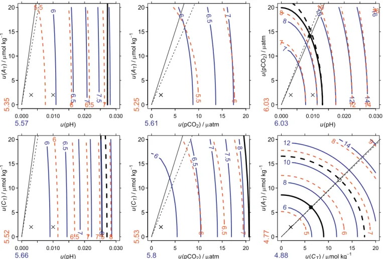
To illustrate how changes in standard uncertainties of a chosen input pair affect a derived variable's combined standard uncertainty, we con-structed a new type of diagram (Fig. 2). This error-space diagram plots contours of the combined standard uncertainty as a function of the range of standard uncertainties in each member of the input pair after prescribing the standard uncertainties for the equilibrium constants as given inTable 1. Thus, it is analogous to the more conventional diagram where contours of a derived variable (e.g., pCO2) are shown as a function of the two members of

an input pair (e.g., ATand CT) except that the axes and contours are the

diagrams can be used to estimate the combined standard uncertainties graphically for the same conditions without further recourse to the un-certainty propagation routines. In addition, they allow users to quickly as-sess how using other methods with different standard uncertainties, which may also differ in cost and convenience, will affect the combined standard uncertainty of a derived variable.

In addition to showing contour lines for the combined standard un-certainty of a derived variable (Fig. 2a), an error-space diagram also in-cludes two other features. It indicates (1) the pair-constants curve (Fig. 2b), along which the constants and the input pair contribute equally and (2) the pair line (Fig. 2c), along which each member of the input pair contributes equally. Inside the pair-constants curve, most of the combined standard uncertainty is from the constants; outside that curve, most of the combined standard uncertainty is from the input pair. Below the pair line, most of contribution to the combined standard uncertainty from the input pair comes from the member indicated on the x-axis label; above the pair line, most of that contribution comes from the member indicated on the y-axis label. The pair line and the pair-constants curve are calculated as described in Appendix C. Generally it will be seen that working to reduce the

uncertainties of members of the input pair by improving methods has a diminishing return on improving the combined standard uncertainty as one crosses the pair-constants curve and moves towards the origin. At the origin of an error-space diagram, the combined standard uncertainty is that at-tributable only to the constants. The basic error-space diagram provides results for one set of input conditions (e.g., AT, CT, T, and S), but up to two

sets of input conditions may be shown if they differ substantially, e.g., average conditions for the tropics and Southern Ocean (Fig. 2d).

As implemented here, error-space diagrams neglect the minute con-tributions from standard uncertainties in T and S, for which oceanographic measurements are usually highly accurate (e.g., u(T)0.01C and u(S)0.01), as well as standard uncertainties from PTand SiT, whose contributions to the

combined standard uncertainty are negligible even in high-nutrient regions. Although PTand SiTsignificantly affect values of computed variables in

high-nutrient waters when ATis a member of the input pair (Orr et al., 2015), the joint contribution of their standard uncertainties to the combined standard uncertainty does not usually exceed 0.1%. Smaller still are the contributions to the combined standard uncertainty from the typical stan-dard uncertainties in T and S mentioned above, which always result in less

Salinity Temper ature (°C) 0.1 0.2 0 10 20 30 40 0.05 0 0 0 0.02 0.005 0.005 −0.01 −0.005 −0.005 0 5 10 15 20 25 30

∆

pK

1

W

aters et al. − Lue

ker et al.

Salinity Temper ature (°C) 0.4 8. 0 0 10 20 30 40 0.1 0.2 0 0 0.02 0.04 _{0.01 0.01} −0.015 −0.01 −0.01 −0.005 −0.005 −0.005 0 5 10 15 20 25 30

∆

pK

2 Salinity Temper ature (°C) 0 0 0.005 0.01 0.01 0.015 0 10 20 30 40 −0.1 −0.05 −0.01 −0.005 _−0.005 −0.2 − 5. 0 0 5 10 15 20 25 30

∆

pK

Salinity Temper ature (°C) 0 0 0 0.005 0.01 0 10 20 30 40 −0.02 5 −0.02 −0.015 −0.01 −0.005 −0.005 −0.005 0 5 10 15 20 25 30

W

aters et al. − Dickson & Millero

Salinity Temper ature (°C) 0 0 0.01 0.01 0.02 0.02 0.03 0 10 20 30 40 − 30 .0 −0.03 −0.02 −0.02 −0.01 −0.01 0 5 10 15 20 25 30 Salinity Temper ature (°C) 0 0 0.01 0.02 0.02 0.03 0.03 0 10 20 30 40 −0.03 −0.02 −0.01 −0.01 0 5 10 15 20 25 30

Fig. 1. Contour plots showing systematic differences between formulations for (left) pK1, (center) pK2, and (right) pK, where K = K1/K2: (top row) formulations of

Waters et al. (2014)minusLueker et al. (2000)and (bottom row) formulations ofWaters et al. (2014)minusDickson and Millero (1987), the latter of which combines the measured data ofHansson (1973)andMehrbach et al. (1973)and extrapolates from salinities of ~20 to zero. Both comparisons are perilous below S~20, which is beyond the valid salinity range of the measured data whether measured byMehrbach et al.(and used inLueker et al.) or byHansson. That low-salinity region is included though as a warning about the large associated uncertainties. In the bottom center and right panels, contour lines converge towards zero difference near

S = 0, e.g., for K2from the largest differences located around S = 5. Red dashed lines are negative, while blue solid lines are positive or zero. (For interpretation of

than a 0.02% relative uncertainty in derived variables. Thus these diagrams focus entirely on the main contributors, i.e., standard uncertainties from the equilibrium constants and from the chosen input pair of carbonate system variables.

To facilitate future production of error-space diagrams by others, we offer an interactive interface available at https://katirg.shinyapps.io/ marineco2errorpropagationfor which users may raise issues or contribute

improvements via GitHub at https://github.com/KatiRG/

marineCO2ErrorPropagation. 3. Results

Packages were evaluated by comparing their numerical derivatives to analytic solutions and automatic derivatives and by comparing their com-bined standard uncertainties computed with a common approach to those from two other methods as well as those from a previous study. Packages were also compared to one another. Subsequently, the new routines from one package were used to characterize combined standard uncertainties as a function of standard uncertainties of input variables for two contrasting ocean regions by means of error-space diagrams.

3.1. Agreement

Comparison first focused on the consistency of computed partial deri-vatives (sensitivities) and combined standard uncertainties among packages, among approaches, and in comparison to previous work. Comparison of these sensitivities among packages reveals that they agree to at least four

significant figures, i.e., within at least 0.01% (Tables 2 and 3).

Results from the seacarb package's numerical derivatives generally agree to at least five significant figures (within 0.001%) with the analytical so-lution from the same package. Results from mocsy's numerical derivatives and its automatic derivatives also agree within at least four significant fig-ures. Overall, the buffer factors calculated from the four packages and from the analytical solutions always agree to better than 0.01%. Similar agree-ment is found for the combined standard uncertainties with packages dif-fering by < 0.008% for computed concentrations and partial pressures and by < 0.03% for ΩAand ΩC(Table 4). Although still small, the differences

for the Ω's are larger because the formulation for the [Ca2+_{]/S ratio differs}

slightly among packages (Orr et al., 2015).

For a historical perspective,Table 5shows our sensitivities and com-bined standard uncertainties calculated with the same input conditions as those fromDickson and Riley (1978). Our K1and K2values are only 0.4%

and 1.2% smaller (when converted to the same pH scale), being calculated followingLueker et al. (2000)as recommended for best practices (Dickson et al., 2007). For the pH-ATand pH-CTinput pairs, calculated sensitivities

generally differ by a few percent at most from those ofDickson and Riley (1978)except that our sensitivities of computed CTand ATto [H+] are up to

36% higher. For the pCO2-ATand pCO2-CTinput pairs, the magnitude of our

computed sensitivities are within 12% of those from Dickson and Riley's estimates, except for our sensitivities of computed ATor CTto input pCO2, K0, and K1, which are up to 36% larger. There is also a sign inconsistency

with the pCO2-ATpair, for which our computed ∂ ln [CO32−]/∂ ln (K2) is

negative while Dickson and Riley's estimate is positive due to a typo in the latter. For the pCO2-pH input pair, all sensitivities are within 5% of those

0 5 10 15 20

u(CT

) / µmol kg

−1

u(

A

T

) /

µmol kg

−1 4.88 6 8 10 12 14

0

5

10

15

20

a

0 5 10 15 20

u(C

T

) / µmol kg

−1

u(

A

T

) /

µmol kg

−1 4.88 6 8 10 12 14

0

5

10

15

20

b

0 5 10 15 20

u(C

T

) / µmol kg

−1

u(

A

T

) /

µmol kg

−1 4.88 6 8 10 12 14

0

5

10

15

20

c

0 5 10 15 20

u(C

T

) / µmol kg

−1

u(

A

T

) /

µmol kg

−1 4.88 4.77 6 8 10 12 14 5 6 7 8 9

0

5

10

15

20

d

Fig. 2. Anatomy of an error-space diagram. As its base, this diagram includes (a) contours of the percent relative combined standard uncertainty of a calculated

variable (blue), in this case ΩA, as a function of the standard uncertainties in the input pair, in this case CT(x-axis) and AT(y-axis). Then in panel (b) is added the pair-constants curve, along which the contribution to the combined standard uncertainty from the input pair is equal to that from the pair-constants, the latter being indicated

by the blue number below the origin. In addition, in panel (c) is added the pair line along which the two members of the input pair contribute equally to the combined standard uncertainty. Finally, panel (d) shows results not only for average surface water of the Southern Ocean (blue), as before, but also for the tropics (red), including the contribution to the combined standard uncertainty from only the constants (red number to the left of the origin). A symbol (x) is also added to indicate an arbitrary reference for the standard uncertainties for the input pair, in this case 2 μmol kg−1_{for each of C}

Tand AT(Table 1). (For interpretation of the references to colour in this figure legend, the reader is referred to the web version of this article.)

from Dickson and Riley. For the AT-CTpair, most sensitivities are lower but

remain within 30% of the Dickson and Riley estimates, except for sensi-tivities to K2of computed [HCO3−] and [CO32−], which are about 4 and 7

times larger. These differences are partly explained by our use of ATversus

Dickson and Riley's use of carbonate alkalinity AC (Sect. 4.1). Despite

roughly consistent sensitivities between the two studies as well as generally comparable contributions to the combined standard uncertainties from the input pair, our overall combined standard uncertainties in Table 5 are usually smaller than those from Dickson and Riley because our default input uncertainties for K1and K2are 25% smaller.

By default, all packages use the Gaussian approach to propagate un-certainties, an approach that assumes no correlation between the standard uncertainties of the two members of the input pair. For comparison, we also implemented the Monte Carlo approach in the errors function of the seacarb package. It too was coded to include no correlation between uncertainties of the input variables. Results from the Monte Carlo approach agree with those from the Gaussian approach, our reference, within the statistics permitted by the number of random samples taken (Fig. 3), an additional input parameter that is specified only for the Monte Carlo approach. Random sample sizes must be as large as 105_{for the Monte Carlo approach to be able} Table 2

Comparison of partial derivatives across packages calculated from surface-ocean global meansa_{for A}

T, CT, T, and S.

[H+_{] pCO}

2 [CO2∗] [HCO3−] [CO32−] ΩA

∂/∂AT

(nmol μmol−1_{) (μatm kg μmol}−1_{) (μmol μmol}−1_{) (μmol μmol}−1_{) (μmol μmol}−1_{) (kg μmol}−1₎

co2sysb _-0.02558196‡ _-1.192136c _{−0.04073334 −0.6310411 0.6717745 0.01037201} Mocsy −0.02558194 −1.192138 −0.04073333 −0.6310401 0.6717725 0.01037431 Ref.d _{−0.02558194 −1.192138 −0.04073333 −0.6310401 0.6717725 0.01037431} Ref.e _{−0.02558201 −1.192140 −0.04073345 −0.6310539 0.6717729 0.01037431} Seacarb −0.02557970 −1.192033 −0.04072973 −0.6310761 0.6718058 0.01037482 Ref.f _{−0.02558003 −1.192046 −0.04073025 −0.6310842 0.6718144 0.01037496} ∂/∂CT

(nmol μmol−1_{) (μatm kg μmol}−1_{) (μmol μmol}−1_{) (μmol μmol}−1_{) (μmol μmol}−1_{) (kg μmol}−1₎

co2sysb _{0.02810982 1.461280 0.04992956 1.584240 −0.6341699 −0.00979141} Mocsy 0.02810980 1.461283 0.04992955 1.584239 −0.6341677 −0.00979357 Ref.d _{0.02810980 1.461283 0.04992955 1.584239 −0.6341677 −0.00979357} Ref.e _{0.02810988 1.461285 0.04992968 1.584255 −0.6341683 −0.00979358} Seacarb 0.02810754 1.461163 0.04992547 1.584277 −0.6342023 −0.00979411 Ref.f _{0.02810790 1.461178 0.04992604 1.584286 −0.6342118 −0.00979425} ∂/∂T

(nmol kg−1_C−1_{) (μatm C}−1_{) (μmol kg}−1_C−1_{) (μmol kg}−1_C−1_{) (μmol kg}−1_C−1_{) (C}−1₎

co2sysb _{0.2525344 12.57638 0.1332509 −0.5848728 0.4516218 0.01716385}

Mocsy 0.2525339 12.57640 0.1332499 −0.5848648 0.4516475 0.01716809

Ref.c _{0.2525339 12.57640 0.1332499 −0.5848648 0.4516475 0.01716809}

Seacarb 0.2525121 12.57521 0.1332345 −0.5849710 0.4517364 0.01717017

∂/∂Sg

(nmol kg−1_{) (μatm) (μmol kg}−1_{) (μmol kg}−1_{) (μmol kg}−1₎

co2sysb _{0.2099016 8.299964 0.2268601 1.004573 −1.231433 −0.03713724}

Mocsy 0.2099018 8.299996 0.2268604 1.004582 −1.231429 −0.03714548

Ref.d _{0.2099018 8.299996 0.2268604 1.004582 −1.231429 −0.03714548}

Seacarb 0.2098768 8.298895 0.2268276 1.004441 −1.231269 −0.03714426

a _{Input conditions: AT = 2300 μmol kg}−1_{, CT = 2000 μmol kg}−1_{, T = 18}◦_{C, S = 35, PT = 0 μmol kg}−1_{, and S iT = 0 μmol kg}−1_. b _{CO2SYS-Matlab}

c _{The first number in the table is for ∂[H+]/∂AT, the second number for ∂pCO2/∂AT, both from the CO2SYS-Matlab package.} d_{Automatic derivative in mocsy (derivauto.f90 routine)}

e _{Analytic derivative in mocsy (buffesm.f90 routine)} f _{Analytic derivative in seacarb (buffesm.R function)}

g _{Since salinity is on the practical salinity scale, no units are given for the denominator of ∂/∂S partial derivatives}

Table 3

Comparison of computed partial derivatives with respect to PTand SiTfor typical surface conditionsa.

[H+_{] pCO}

2 [CO2∗] [HCO3−] [CO32−] ΩA

∂/∂PT

(nmol μmol−1_{) (μatm kg μmol}−1_{) (μmol μmol}−1_{) (μmol μmol}−1_{) (μmol μmol}−1_{) (kg μmol}−1₎

co2sysb _{0.02935462 1.368130 0.04674678 0.7009685 −0.7477153 −0.01154451}

Mocsy 0.02935621 1.368207 0.04674931 0.7010073 −0.7477555 −0.01154773

Ref.c _{0.02935621 1.368207 0.04674931 0.7010073 −0.7477555 −0.01154773}

Seacarb 0.02935388 1.368098 0.04674557 0.7010528 −0.7477984 −0.01154839

∂/∂SiT

(nmol μmol−1_{) (μatm kg μmol}−1_{) (μmol μmol}−1_{) (μmol μmol}−1_{) (μmol μmol}−1_{) (kg μmol}−1₎

co2sysb _{0.001069476 0.04984502 0.001703124 0.02553836 −0.02724148 −0.0004206009}

Mocsy 0.001069695 0.04985535 0.001703473 0.02554362 −0.02724705 −0.0004207814

Ref.c _{0.001069695 0.04985535 0.001703473 0.02554362 −0.02724705 −0.0004207814}

Seacarb 0.001069679 0.04985458 0.001703446 0.02554693 −0.02725038 −0.0004208327

a _{Input conditions as inTable 2except that PT = 2.0 μmol kg−1, and S iT = 60 μmol kg−1.} b _{CO2SYS-Matlab}

to routinely obtain combined standard uncertainties that agree with those from the default Gaussian approach within < 1%. With random samples of that size, the computation time for the Monte Carlo approach is 10 times longer than the Gaussian approach for the pCO2-pH pair but 440 times

longer for the AT-CTpair based on our implementation in seacarb.

The third approach, Method of Moments, is unlike the others in that its calculated combined standard uncertainties can be affected by a user-spe-cified correlation (r) between the standard uncertainties of the two members of the input pair. With r = 0, the Method of Moments matches results from the Gaussian approach; with nonzero values of r (between −1 and +1), the combined standard uncertainties are affected variously, depending on the computed variable and the input pair as well as the value of r. For instance, for the pCO2-pH pair, by assuming a perfect correlation (r = 1) between the

uncertainties in pCO2 and [H+], the overall propagated uncertainty in

computed [CO32−] is 24% less than with no correlation (Table 6). There is a

reduction because of the negative sign of the covariance term (last term in Eq.(1)), i.e., twice the product of the two sensitivities, the individual un-certainties, and the correlation coefficient (between the two uncertainties):

+ + + p u p u r p 2 [CO ] CO [CO ] [H ] ( CO ) ([H ]) ( CO , [H ]) 3 2 2 3 2 2 2 (4) The covariance term is negative because the two standard uncertainties are positive (by definition), the two sensitivities are opposite in sign (e.g., Table 5c), and r(pCO2,[H+]) is positive. Thus combined standard

certainties can be affected by correlations between the standard un-certainties of the two members of the input pair. However, the correlation between the standard uncertainties is not the same as a correlation between the measurements themselves. For uncertainty propagation, the interest is in the correlation between standard uncertainties of input variables, not be-tween the values of the input variables themselves. If there is a measure-ment uncertainty that is common to both members of the input pair, then that commonality should be accounted for explicitly. Correlation between standard uncertainties of other input variables such as K1and K2remains

possible but requires further investigation. Hence adding room for those additional correlations in the uncertainty propagation routines is left to future work.

3.2. Error space

To quantify combined standard uncertainties more generally and assess the potential for improvement, we used our errors function from the seacarb package to provide data for error-space diagrams (Sect. 2.5), which show how combined standard uncertainties in derived variables are affected by the range of possible uncertainties in input variables. Uncertainties were propagated for five calculated variables [CO32−], ΩA, pCO2, [H+], and

[HCO3−], along with the ratio of the latter two [HCO3−]/[H+], all as a

function of a range of standard uncertainties in each member of six input

pairs (pH-AT, pH-CT, pCO2-AT, pCO2-CT, pCO2-pH, and AT-CT). The

com-puted combined standard uncertainties were compared using error-space diagrams drawn for each input pair and each computed variable (Figs. 4–11).

3.2.1. [CO32−]

Error-space diagrams for [CO32−] emphasize that its combined standard

uncertainty is lowest when calculated with the AT-CTinput pair and highest

when calculated with the pCO2-pH pair (Fig. 4). Each member of the AT-CT

pair contributes nearly equally to the combined standard uncertainty of [CO32−] when their standard uncertainties are identical because the

sen-sitivities of [CO32−] to ATand CThave similar magnitudes. With identical

sensitivities for each member of the input pair, an error-space diagram would be perfectly symmetrical (Eq. (1)), an ideal case that is nearly reached for [CO32−] as well as most other variables computed from the AT -CTpair. For that pair, the pair-constants curves occur at about 2% relative

uncertainty in [CO32−] for surface waters of both the tropics and the

Southern Ocean. For other pairs, relative combined standard uncertainties in [CO32−] are larger, particularly for the pCO2-pH input pair, and

con-tributions of the standard uncertainties from the two members of the input pair are less symmetric. Given state-of-the-art standard uncertainties (Table 1), if pH is a member of the input pair, its contribution to the combined standard uncertainty is substantially larger than that from the other member, as revealed by the position of the reference points (crosses) which sit well below the pair line. Likewise, when pCO2is a member of the

input pair, its contribution is larger except when the other member is pH. In the error-space diagrams, the much heavier weight of pH or pCO2(x axis)

when paired with ATor CT(y axis) is also manifested by near-vertical lines

for overall propagated uncertainty. For all pairs, current state-of-the-art standard uncertainties in each of their members place the corresponding propagated uncertainty within the pair-constants curve, where the un-certainty from the constants outweighs the unun-certainty from the input pair. Thus further improvements to methods to reduce their measurement un-certainties would do little to reduce the combined standard uncertainty, given the substantial propagated uncertainty from the constants. For ex-ample, a threefold reduction of the standard uncertainty in pH from 0.01 to 0.003 lowers the combined standard uncertainty of [CO32−] by only a

factor of one-seventh with the pH-ATand pH-CTpairs and one-third with the pCO2-pH pair.

3.2.2. ΩA

For ΩA, error-space diagrams are similar to those for [CO32−], except

that relative combined standard uncertainties are typically a few percent larger and pair-constants curves are farther from the origin, simply due to the standard uncertainty in KA(u(pKA) = 0.02), a constant (solubility

pro-duct) that only affects computed ΩA(Fig. 5). The pair-constants curve for

the AT-CTpair occurs at about 7% relative combined standard uncertainty

for both regions, i.e., at a value that is more than twice that seen for

Table 4

Combined standard uncertainties in variables computed with the AT-CTpair at typical surface conditionsa.

[H+_{] [CO}

2∗] fCO2 pCO2 [HCO3−] [CO32−] ΩA ΩC

(nmol kg−1_{) (μmol kg}−1_{) (μatm) (μatm) (μmol kg}−1_{) (μmol kg}−1₎ Without standard uncertainties from the constants

CO2SYS-Excel 0.07668398 0.12995259 3.7900747 3.8032995 3.4135224 1.8539528 0.02862451 0.04426536 CO2SYS-Matlab 0.07668398 0.12995259 3.7900747 3.8032994 3.4135224 1.8539528 0.02862451 0.04426536 Mocsy 0.07669003 0.12996267 3.7903686 3.8036035 3.4135222 1.8539595 0.02863104 0.04427546 Seacarb 0.07668414 0.12995262 3.7900755 3.8033093 3.4136038 1.8540405 0.02863230 0.04427739

With default standard uncertainties from the constants

CO2SYS-Excel 0.19429498 0.32911625 9.6994199 9.7332644 4.4247168 3.2612783 0.15578845 0.24091348 CO2SYS-Matlab 0.19429498 0.32911625 9.6994199 9.7332642 4.4247168 3.2612783 0.15578845 0.24091348 Mocsy 0.19430788 0.32913860 9.7000746 9.7339444 4.4247421 3.2613327 0.15581821 0.24095949 Seacarb 0.19429739 0.32911714 9.6994403 9.7333078 4.4247272 3.2612654 0.15582641 0.24097219 a _{Input conditions ( ± u): AT = 2300 ± 2 μmol kg−1, CT = 2000 ± 2 μmol kg−1, T = 18 ± 0◦C, S = 35 ± 0, PT = 2.0 ± 0.1 μmol kg−1, and S} iT = 60 ± 4 μmol kg−1.

Table 5

Relative sensitivities of output to input (∂y/y)/(∂x/x) and propagated percent relative combined standard uncertainties ucfor six input pairsa.

(a) Input (pH-ATpair) sensitivities uc(%)c

Output [H+_{] CT K0 K1 K2 (i) (ii)}

[CO2∗] b1.249 b1.048 −1.000 −0.212 2.9 3.5 [HCO3−] 0.249 1.048 −0.212 0.7 1.0 [CO32−] −0.751 1.048 0.788 1.8 3.3 CT 0.136 1.048 −0.005 −0.094 0.5 0.6 pCO2 1.249 1.048 −1.000 −1.000 −0.212 2.9 3.5 ΩA −0.751 1.048 0.788 1.8 5.6

(b) Input (pH-CTpair) sensitivities σ (%)

Output [H+_{] CT K0 K1 K2 (i) (ii)}

[CO2∗] 1.113 1.000 −0.995 −0.118 2.6 3.2 [HCO3−] 0.113 1.000 0.005 −0.118 0.6 0.7 [CO32−] −0.887 1.000 0.005 0.882 2.1 3.7 AT −0.130 0.955 0.005 0.090 0.6 0.6 pCO2 1.113 1.000 −1.000 −0.995 −0.118 2.6 3.2 ΩA −0.887 1.000 0.005 0.882 2.1 5.9

(c) Input (pCO2-pH pair) sensitivities σ (%)

Output [H+_{] pCO} 2 K0 K1 K2 (i) (ii) [CO2∗] 1.000 1.000 2.0 2.1 [HCO3−] −1.000 1.000 1.000 1.000 3.0 3.5 [CO32−] −2.000 1.000 1.000 1.000 1.000 5.0 6.4 AT −1.192 0.954 0.954 0.954 0.203 3.3 3.8 CT −1.113 1.000 1.000 0.995 0.118 3.3 3.7 ΩA −2.000 1.000 1.000 1.000 1.000 5.0 7.8

(d) Input (AT-CTpair) sensitivities uc(%)

Output AT CT K0 K1 K2 (i) (ii)

[CO2∗] −8.536 9.146 0.000 −0.955 0.652 2.0 3.5 [HCO3−] −0.875 1.835 0.000 0.009 −0.040 0.4 0.4 [CO32−] 6.787 −5.476 0.000 −0.027 0.268 1.3 1.7 [H+_{] −7.661 7.311 0.000 0.036 0.692 1.7 3.0} pCO2 −8.536 9.146 −1.000 −0.955 0.652 2.0 3.5 ΩA 6.787 −5.476 0.000 −0.027 0.268 1.3 4.9

(e) Input (pCO2-ATpair) sensitivities σ (%)

Output AT pCO2 K0 K1 K2 (i) (ii)

[CO2∗] 1.000 1.000 2.0 2.1 [HCO3−] 0.838 0.200 0.200 0.200 −0.171 0.5 0.9 [CO32−] 1.676 −0.599 −0.599 −0.599 0.659 1.4 2.9 [H+_{] −0.838 0.800 0.800 0.800 0.171 1.6 2.3} CT 0.933 0.109 0.109 0.104 −0.071 0.4 0.5 ΩA 1.676 −0.599 −0.599 −0.599 0.659 1.4 5.4

(f) Input (pCO2-CTpair) sensitivities σ (%)

Output CT pCO2 K0 K1 K2 (i) (ii)

[CO2∗] 1.000 1.000 2.0 2.1 [HCO3−] 0.898 0.102 0.102 0.107 −0.107 0.5 0.6 [CO32−] 1.795 −0.795 −0.795 −0.786 0.786 1.8 3.6 [H+_{] −0.898 0.898 0.898 0.893 0.107 1.9 2.5} AT 1.071 −0.117 −0.117 −0.112 0.076 0.6 0.7 ΩA 1.795 −0.795 −0.795 −0.786 0.786 1.8 5.8

a _{For comparison to Table II ofDickson and Riley (1978)calculated with the same input: A}

T= 2355 μmol kg−1computed from AC= 2248 μmol kg−1, CT= 2017

μmol kg−1_{, pH = 8.10 on the total scale computed from pH = 8.25 on the NBS scale using Eq. (15) fromLueker et al. (2000), pCO}

2= 350 μatm, T = 25◦C, and

S = 35, having zero standard uncertainty in T and S, a standard uncertainty of 0.01 in pH, a relative standard uncertainty of 2% for pCO2, and relative standard

uncertainties of 0.4% for ATand 0.5% for CTexcept for the AT-CTpair where the latter two standard uncertainties were instead 0.1 and 0.2%. Combined standard uncertainty estimates fromDickson and Riley (1978)were based on precision at that time, not accuracy.

b _{The first number in the table is for ∂ ln[CO}∗

2]/∂ ln[H+], the second for ∂ ln[CO∗2]/∂ ln AT.

c _{The final two columns list combined standard uncertainties computed considering standard uncertainties in (i) only the input pair and (ii) the input pair and the} equilibrium constants (total uncertainty).

[CO32−]. Because pair-constants curves are more distant from the origin

owing to the relatively larger contribution to the combined standard un-certainty from the constants (due to KA), improving standard uncertainties

of the input pair would have even less effect on the combined standard uncertainty. Yet that also means that reducing methodological uncertainty requirements for the input pair from the state-of-the-art constraints, which are well under the pair-constants curve, results in little worsening of overall propagated uncertainties. For instance, a fivefold increase from the cur-rently smallest possible uncertainties for the input pair (crosses inFig. 5) adds < 1% to the overall propagated relative uncertainty in ΩAfor input

pairs where the pair-constants curve is either near the edge or outside of the plot domain (pH-AT, pH-CT, pCO2-AT, and pCO2-CTpairs).

3.2.3. pCO2and [CO2∗]

Three of the six input pairs include pCO2as a member, while for the

three others it is calculated. For the latter three, the two that include pH as a member of the input pair have combined standard uncertainties in pCO2

that vary only as a function of u(pH) throughout most of the plot domain (Fig. 6). Those close ties are explained by the near-linear relationship be-tween [CO2∗] and [H+] (Orr, 2011;Kwiatkowski and Orr, 2018) and the

relative insensitivity to likely uncertainties in the opposing member of each input pair (ATor CT). In those two plot domains, curvature is obvious only at

lower u(pH) and higher u(AT) or u(CT) (above 10 μmol kg−1). For the

remaining AT-CTpair, relative combined standard uncertainties of pCO2are

nearly symmetrical with respect to each member as they are for [CO32−],

but with pCO2they are larger and the pair-constants curves are about twice

as far from the origin. Thus, changes in standard uncertainties of the input pair from the same state-of-the-art reference have even less effect on the combined standard uncertainty of pCO2relative to that for [CO32−]. That

difference is driven by the relative contribution to the combined standard uncertainty from the constants being larger for pCO2than for [CO32−]. For pCO2, increasing standard uncertainties of ATand CTfrom 2 to 10 μmol kg −1_{results in an increase in the percent relative combined standard}

un-certainty from about 3 to 6% in the tropics. For the same three pairs, re-lative combined standard uncertainties in [CO2∗] (Fig. 7) are visually

in-distinguishable from those for pCO2(Fig. 6). When pCO2is a member of the

input pair, it may be used to directly compute [CO2∗], knowing only K0and

that the relationship is linear. For example at u(pCO2) = 10 μatm, the

percent relative standard uncertainty in [CO2∗] is about 3% for surface

waters of both the tropics and the Southern Ocean based on their average surface composition given inFig. 4.

3.2.4. pH and [H+_]

Error-space diagrams showing absolute combined standard un-certainties in pH (Fig. 8) actually represent a relative change in [H+_{]. They}

may be converted to percent relative combined standard uncertainties in [H+_{] simply by multiplying by c = 2.3 × 100. The resulting error-space}

diagrams for [H+_{] (Fig. 9) are analogous to those for pCO}

2(Fig. 6),

al-though input pairs with pH are excluded in the former and pairs with pCO2

are excluded in the latter, as described above. Owing to the near-linear relationship between these two calculated variables, relative combined standard uncertainties and pair-constants curves for [H+_{] computed from}

the pCO2-AT and pCO2-CT input pairs closely resemble those for pCO2

computed from the pH-ATand pH-CTinput pairs, respectively. The

corre-sponding error-space diagrams for [H+_{] and pCO}

2each computed from the AT-CTpair also closely resemble one another.

3.2.5. [HCO3−]

Unlike previous error-space diagrams, those for [HCO3−] differ in

sev-eral ways (Fig. 10). First, the percent relative combined standard un-certainties are around an order of magnitude lower than those for other variables, e.g., < 1% over most of the plot domain at least for the Southern Ocean, except for the pCO2-pH pair. Second, there is much less symmetry Fig. 3. Percent relative combined standard uncertainty of carbonate ion concentration computed with the Gaussian approach (blue dotted line) vs. the Monte Carlo

approach (black dots with error bars). The Monte Carlo approach requires an input parameter to specify the number of iterations (runs). That approach was used with the same input, altering only the number of iterations to make five separate estimates of the propagated uncertainty (runs = 10n_{, where n = 2, 3, 4, 5, 6). That} exercise was then repeated 9 more times for each case to compute statistics, i.e., mean ± 1 standard deviation (shown as the filled symbols and error bars). In both approaches, [CO32−] is computed from the following conditions ( ± u): pCO2= 400 ± 2 μatm, pH = 8.100 ± 0.005 (total scale), S = 35 ± 0, T = 18 ± 0 C, PT= 2.0 ± 0.1 μmol kg−1, and SiT= 60 ± 4 μmol kg−1. (For interpretation of the references to colour in this figure legend, the reader is referred to the web version of this article.)

Table 6

Relative change in combined standard uncertainty (%) that would result from correlation between the uncertainties of pCO2and pH.

r [HCO3−] [CO32−] CT AT ΩA

0 0 0 0 0 0

0.5 −20 −11 −19 −18 −11

than seen for previous error-space diagrams between members of the AT-CT

pair, while there is greater symmetry for the pCO2-pH pair. The former is

explained by the high sensitivity of computed [HCO3−] to CTas also evident

in the error-space diagrams for pH-CTand pCO2-CT. Third, there are larger

differences in patterns of percent relative combined standard uncertainties between the two regions for the four pairs where either pH or pCO2is a

member.

3.2.6. [HCO3−]/[H+]

The [HCO3−]/[H+] ratio (Fig. 11) is a derived variable that has been

proposed as being potentially physiologically more relevant to determining the gross calcification rate than either ΩAor ΩCbecause [HCO3−]

stimu-lates calcification while [H+_{] inhibits it (Bach, 2015). This derived quantity}

is also known as the substrate-to-inhibitor ratio (SIR) (Fassbender et al., 2016b). With the pCO2-pH pair, overall propagated relative uncertainties of

SIR are much like those for [HCO3−]; for other pairs, they resemble those

for [H+_{]. The reason is that the percent relative combined standard}

un-certainties in [H+_{] are larger than those for [HCO}

3−] with all pairs except

for pCO2-pH. Given state-of-the-art total standard uncertainties for the four

measured variables (Table 1), AT-CTis the worst pair to use to compute SIR

even though the pCO2-pH pair is the poorest combination to compute

[HCO3−]. The best combinations for SIR are the four remaining pairs: pH-AT, pH-CT, pCO2-AT, and pCO2-CT. In the first two of those pairs, where pH

is measured not calculated, it might be expected that combined standard uncertainties for SIR would be lower because u(HCO3−)/[HCO3−] ≪ u

([H+_])/[H+_{]. That would be the result if one considered only our random}

component for the standard uncertainty in pH of 0.003 (Table 1). However, using the total standard uncertainty of 0.01 raises the combined standard uncertainty in SIR to the same level as for the two other pairs where pCO2is

a member.

Although we provide error-space diagrams for SIR, doing so appears to offer little new insight. The patterns of SIR's combined standard un-certainties follow those for [CO32−] (Fig. 4) given that SIR = [CO32−]/K2.

Likewise they follow those for ΩA(Fig. 5), when [Ca2+] is not manipulated,

because ΩA= [Ca2+][CO32−]/KA. Given these proportionalities, SIR does

not provide independent information. 4. Discussion

To place results in context, let us now look further into sensitivities, approach suitability, sources of uncertainties, impacts of covariance, and uncertainty criteria for large-scale measurement programs.

0.000 0.010 0.020 0.030 u(pH) u( AT ) / µmol kg −1

3.13

2.71

3.2

3.5

4

5

6

2.8

3.2 3.5

4

5

0 5 10 15 20 0 5 10 15 20 u(pCO2) / µatm u( AT ) / µmol kg −1

3.21

2.51

3.5

4

4.5

5

5.5

3

5.

3

4

0 5 10 15 20 0.000 0.010 0.020 0.030 u(pH) u(pCO 2 ) / µatm

3.89

3.89

5

6

7

6

8

4

5

6

7

01

21

41

0 5 10 15 20 0.000 0.010 0.020 0.030 u(pH) u( CT ) / µmol kg −1

3.29

3.04

3.5

4

5

6

7

3.1

3.5 4

5

6

0 5 10 15 20 0 5 10 15 20 u(pCO2) / µatm u( CT ) / µmol kg −1

3.53

3.05

4

4.5

5

5.5

6

6.5

3.5

4

5.

4

5

5.5

0 5 10 15 20 0 5 10 15 20 u(CT) / µmol kg−1 u( AT ) / µmol kg −1

1.6

1.24

2

4

6

8

10

12

14

2

4

6

0 5 10 15 20

Fig. 4. Error-space diagrams of the percent relative combined standard uncertainty in [CO32−] computed from six input pairs as a function of standard uncertainties in each pair's two members. Input pair members are indicated by the x- and y-axis labels. Combined standard uncertainties depend on the composition of seawater. Blue solid lines indicate average conditions for surface waters of the Southern Ocean (AT= 2295 μmol kg−1, CT= 2155 μmol kg−1, temperature T = − 0.49 C, and salinity S = 33.96), while red dashed lines indicate average conditions for tropical surface waters (AT= 2300 μmol kg−1, CT= 1960 μmol kg−1, temperature

T = 27.01 C, and salinity S = 34.92). Crosses indicate the state-of-the-art standard uncertainty for each member of the input pair (next to last column inTable 1) as

well as the random component of the standard uncertainty for pH (previous column). Black lines indicate the pair line (thin) and pair-constants curve (thick) for both regions (Southern Ocean, solid; tropics, dashed); at their intersections lie the pair-constants midpoints (Southern Ocean, filled circle; tropics, open circle). Pair-constants midpoints fall outside of the plot domain for four of the pairs: pH-AT, pH-CT, pCO2-AT, and pCO2-CT. Colored numbers in the margin near each panel's origin indicate the contribution to the overall propagated uncertainty from the constants alone for the Southern Ocean (blue) and the tropics (red). (For interpretation of the references to colour in this figure legend, the reader is referred to the web version of this article.)