Experimental and theoretical studies of secondary bending of bonded composite butt joints in tension

Publisher’s version / Version de l'éditeur:

Collection of Technical Papers : AIAA/ASME/ASCE/AHS/ASC Structures,

Structural Dynamics and Materials Conference, 2010-04-12

READ THESE TERMS AND CONDITIONS CAREFULLY BEFORE USING THIS WEBSITE.

https://nrc-publications.canada.ca/eng/copyright

Vous avez des questions? Nous pouvons vous aider. Pour communiquer directement avec un auteur, consultez la première page de la revue dans laquelle son article a été publié afin de trouver ses coordonnées. Si vous n’arrivez Questions? Contact the NRC Publications Archive team at

PublicationsArchive-ArchivesPublications@nrc-cnrc.gc.ca. If you wish to email the authors directly, please see the first page of the publication for their contact information.

NRC Publications Archive

Archives des publications du CNRC

This publication could be one of several versions: author’s original, accepted manuscript or the publisher’s version. / La version de cette publication peut être l’une des suivantes : la version prépublication de l’auteur, la version acceptée du manuscrit ou la version de l’éditeur.

For the publisher’s version, please access the DOI link below./ Pour consulter la version de l’éditeur, utilisez le lien DOI ci-dessous.

https://doi.org/10.2514/6.2010-3103

Access and use of this website and the material on it are subject to the Terms and Conditions set forth at

Experimental and theoretical studies of secondary bending of bonded

composite butt joints in tension

Li, Gang; Johnston, Andrew; Yanishevsky, Marko; Bellinger, Nicholas C.

https://publications-cnrc.canada.ca/fra/droits

L’accès à ce site Web et l’utilisation de son contenu sont assujettis aux conditions présentées dans le site LISEZ CES CONDITIONS ATTENTIVEMENT AVANT D’UTILISER CE SITE WEB.

NRC Publications Record / Notice d'Archives des publications de CNRC:

https://nrc-publications.canada.ca/eng/view/object/?id=2d270ba9-6935-421e-9dc9-51fdb2422980

https://publications-cnrc.canada.ca/fra/voir/objet/?id=2d270ba9-6935-421e-9dc9-51fdb2422980

1

Experimental and Theoretical Studies of Secondary Bending

of Bonded Composite Butt Joints in Tension

Gang Li,1 Andrew Johnston,2 Marko Yanishevsky,3 and Nicholas C. Bellinger,4

National Research Council Canada, 1200 Montreal Road, Ottawa, ON, Canada K1A 0R6

The deformation of adhesively bonded composite butt joints in tension was investigated experimentally, theoretically, and numerically. Two single-strap butt joints were tested, the only difference between them being the thickness of the doubler. The case 1 joint was fabricated using identical laminated composite panels for both the adherends and the doubler, while the case 2 joint had a 50% thicker doubler. Expressions for the effective Young’s modulus and bending stiffness for the composite butt joint were derived under both plane strain and plane stress conditions. Joint deformation in the out-of-plane direction and longitudinal elongation could then be theoretically analyzed. A theoretical model for the joint elongation was developed, and an approach was proposed to deal with the strain discontinuity at the overlap end of the joint using the derived theoretical method. Three-dimensional finite element models were created for the analysis of the unit-width joints under a plane strain condition. Good agreement in the predicted joint deformation (deflection, elongation, and strain) was achieved between the three methods. The results suggested that joint bending under both plane strain and plane stress condition should be studied so that the actual strain range in high bend areas (overlap edge regions) can be determined. Expressions for the four basic parameters in the coupled adhesive stress differential equations were also developed and two strategies were presented to explore the complete closed-form adhesive stress solutions in a general composite butt joint configuration. Finite element results showed that peak adhesive stresses were located at the inner overlap edge, and suggested that appropriate reinforcement should be made in this region to ensure a sufficient safety margin.

Nomenclature

xx

E and D _x Effective Young’s modulus and bending stiffness of the laminates

[ ]

M and

[ ]

N Unit width moment and in-plane force matrices of laminated composites

11

k , k12, and k22 Elements in the compliance matrix of the in-plane constitutive relation for a classic

Euler-Bernoulli composite beam provided there are no transverse loads

Aiand Bi Integration constants (i=1, 2, 3) in the joint deflection expressions 2c Bondline length between one adherend and doubler

L Outer unbonded adherend length. l

∆ Joint elongation

0

2L Length of the inner unbounded (or unoverlapped) doubler gap section

t1 and t2 Thickness of the adherend and doubler.

T Unit width joint remote tensile force (N/mm) i

µ

Joint parameter (

i

=

1, 2, 3)

1

Associate Research Officer, Structures and Materials Performance Laboratory, Institute for Aerospace Research, Gang.Li@nrc-cnrc.gc.ca. Member AIAA.

2

Group Leader, Composites and Novel Airframe Materials, Structures and Materials Performance Laboratory, Institute for Aerospace Research.

3

Senior Research Officer, Structures and Materials Performance Laboratory, Institute for Aerospace Research.

4

Group Leader, Aerospace Structures, Structures and Materials Performance Laboratory, Institute for Aerospace Research.

51st AIAA/ASME/ASCE/AHS/ASC Structures, Structural Dynamics, and Materials Conference<BR> 18th

12 - 15 April 2010, Orlando, Florida

AIAA 2010-3103

η Adhesive layer thickness

Eaand Ga Adhesive Young’s modulus and shear modulus

a

σ and τ_a Adhesive peel and shear stresses

1

a , a₂, b₁, and b₂ Four basic parameters in the adhesive stress differential equations

I. Introduction

IBRE reinforced composite primary and secondary aircraft structures have the potential to achieve the same strength and stiffness as conventional metallic structures, but at substantially lower weight. Quasi-isotropic laminated composite panels are usually used in aircraft applications,1-4 since these types of layups maintain satisfactory strength in both longitudinal and hoop directions. A recent high-profile example of the rapid expansion of the use of composites in commercial aircraft is the Boeing 787, which includes composite fuselage barrel sections as large as 6 m in diameter and 15 m long.5 This aircraft is to have its entire fuselage structure assembled by joining together several pre-cured one-piece barrel sections. To accomplish this in an efficient and cost effective manner, the composite joints used to attach these structures will be critical. One possible joint option is the single-strap butt joint configuration. With recent achievements in adhesive and bonding technologies, bonded joints can be both lighter and more cost effective than equivalent bolted or riveted joints. As such, joints with high modulus, high strength adhesives have the potential to have much higher static strengths than bolted joints.4 To supplement adhesive bonding, additional mechanical fasteners can be introduced to enhance structural integrity using a hybrid (bonded and bolted) attachment approach. In order to use this approach, understanding the deformation behaviour of the bonded butt joints is essential. This is the subject of the current study.

The single-strap butt joint is actually fabricated by attaching two single-lap joints end to end.6-8 In this configuration, the joint inner overlap edge will experience much greater bending moments than the outer overlap end when the joint is loaded in tension as a result of secondary bending.9

A recent survey of open literature on bonded composite joints,2, 4, 8-14 showed that: (i) limited experimental data is available on bonded butt joint configurations in tension;14 (ii) a theoretical analysis of laminated composite beams in bending has not been carried out simultaneously for both plane strain and plane stress conditions;9, 10, 15-17 (iii) the difference between parameters such as the effective Young’s modulus, bending stiffness and the obtained strains induced by these two conditions has not been studied9, 10, 15-17 and (iv) no papers were found that theoretically estimate the strain at the overlap end region.

In this paper, deformation of an adhesively bonded composite single-strap butt joint configuration in tension was investigated, addressing the knowledge gap identified in the literature survey. Two different cases of single-strap butt joints were tested. The only feature that was different between the cases was the thickness of the doubler. The case 1 joint was fabricated using identical thickness laminated composite panels for both the adherends and the doubler, while the doubler in the case 2 joint was 50% thicker than that used in the case 1 joint.

The carbon fibre laminates were laid up using an automated fibre placement (AFP) machine at the National Research Council Canada Institute for Aerospace Research, Aerospace Manufacturing Technology Centre located in Montreal, Quebec. Joint dimensions were determined according to a previous study.9 Joint elongation between the cross-heads of a load frame was measured during loading as were strains at key positions, using strain gauges. In addition to experimental measurements, the following theoretical explorations were carried out: (i) expressions were derived for the effective Young’s modulus and bending stiffness for the composite joint under both plane strain and plane stress conditions; (ii) a model was developed to predict the joint elongation; (iii) an approach was devised to eliminate the strain discontinuity at the overlap end in the doubler; and (iv) two strategies were developed to explore the complete closed-form adhesive stress solutions for bonded composite butt joint with different adherends and doublers.18,19 Geometrically nonlinear finite element analyses (FEA) were also carried out for a complete insightful study with both experimental and theoretical methods.

The main objectives of the work presented in this paper are to: (i) obtain useful experimental data for these joints; (ii) evaluate the impact of using plane strain and/or plane stress assumptions on the strain analysis using theoretical methods; and (iii) provide a relevant theoretical model to study joint deformation, which could be used to support further work on assessing composite joint designs.

F

II. Experimental Details

A. Joints and Strain Measurement

A total of four strain-gauged joints were tested to enable comparison between theoretical, FE, and experimental results; n = 2 case 1 and n =2 case 2 joints. Carbon fibre laminates were laid up using an automated fibre placement (AFP) machine and then cured in an autoclave. The layup sequence for all joint adherends was

_[

45/−45/0/90

_]

_2s. The measured nominal thickness of this 16-layer laminate was 2.24 mm. The butt joints were assembled and cured at the panel level, then cut into coupons with a width of 25.4 mm width. The doubler layup sequence was

[

45/−45/0/90

]

2s for case 1 joints, and

[

45/−45/0/90

]

3s for case 2 joints. The thicker doubler using the 24-layer

laminate was 3.36 mm in thickness. The material properties for the laminae of CYCOM 5276-1 T40-800 145/35 (Cytec Engineered Materials) used in this work were as follows: E11= 145 GPa, E22= 8.9 GPa, v12= 0.31, and

=

12

G 4.5 GPa (this data was derived from tests on laminated sheet coupons conducted as part of this work).

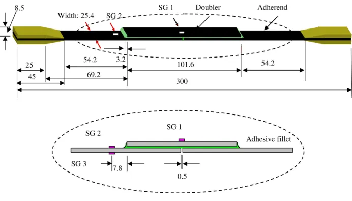
The final joint dimensions and strain gauge arrangements are shown in Figure 1. The inner gap between adherends in the butt joint was approximately 0.5 mm and the adhesive layer thickness was approximately 0.17 mm. An elastic modulus of Ea = 3 GPa and a Poisson’s ratio of va = 0.32 were assumed for the FM300 film adhesive, based on literature for similar adhesives. Tapered end tabs made from 3.18 mm thick FR4 fibreglass sheet were bonded to the coupons using Hysol room temperature cure paste type adhesive EA9396. Three strain gauges (CEA-06-062UW-350, Measurements Group, Inc., North Carolina) with gauge factor of 2.13 ± 0.5% were mounted on each joint in the longitudinal direction. Strain gauge 1 was used to detect the strains at the centre area of the doubler outer surface. Strain gauges 2 and 3 were at the same longitudinal position (7.8 mm from the overlap end) with one installed on the upper surface and the other installed on the lower surface of the same outer adherend. Strain gauge data was used to validate the results of the theoretical analyses.

Figure 1. The bonded composite single-strap butt joint specimen design, and three strain gauge (SG) positions (all dimensions in mm).

SG 3 7.8 SG 2 SG 1 0.5 Adhesive fillet 69.2 101.6 Width: 25.4 Doubler Adherend 300 45 25 54.2 8.5 3.2 54.2 SG 1 SG 2

B. Loading Condition and Data Acquisition

The adhesively bonded composite butt joints were loaded in tension using an MTS load frame equipped with a 22.5 kN load cell (model number 5631 and serial number 611.21A-01). Tensile load was applied at a rate of 2 kN/min up to a maximum load of 5.5 kN, after which point the specimens were unloaded. The joints were loaded and unloaded in this manner a total of three times. The maximum load corresponded to a remote tensile stress of approximately 97 MPa, well within the elastic range for the adherend and doubler. A linear elastic response was also assumed for the adhesive in order to simplify the subsequent theoretical analyses, an approach widely used by a number of researchers.6-9 Notwithstanding the well-known associated compliance issues, joint elongation between the two cross-heads was used to assess joint deformation since an LVDT that could cover the entire overlap section was not available.

III. Theoretical Formulations for Composite Joint Bending Analysis

Under most conditions, the composite adherend and doubler should behave in a linear elastic manner, while the adhesive may exhibit elastic as well as viscoelastic and/or nonlinear properties. Fully capturing material nonlinearities would make an exact analytical treatment of the structural and material problems very complicated. Therefore, linear elastic response in adherend, doubler, and adhesive was assumed in the theoretical analyses in this section. Furthermore, a simplified joint configuration without consideration of the adhesive fillet was used. Peak adhesive stress is usually located at the overlap end with the greatest magnitude being at the butt joint inner edge.18 Joint bending deformation and adhesive stress variation patterns and magnitude are critical in the joint analysis. Good design can effectively reduce both the joint secondary bending and the adhesive stress magnitude. In this section, relevant theoretical preparations for analysis of the bonded butt laminated joint structures were conducted, which were then used to theoretically predict joint deformation, force (tension, shear, and bending) conditions at the overlap ends, and to further identify the adhesive stresses. In this manner, better joint analysis could be achieved.

A. Theoretical Formulations for Composite Laminate Bending Analysis

For the classic Euler-Bernoulli beam, where there are no transverse loads, the in-plane constitutive relationship can be simplified from the constitutive equation for anisotropic composite laminates,15 by keeping only relevant strains and forces as:

= x x x x M N k k k k 22 12 12 11 0 κ ε (1a) where k11, k12, and k22 are to be determined compliance elements. They can be identified under both plane strain (cylindrical bending) and plane stress (classic beam) conditions. For symmetric and balanced laminates, the term k12 is zero. The effective or equivalent Young’s modulus, Exx, and bending stiffness, Dx, of the laminate can then be expressed as: 11 1 k t Exx = (1b)

( )

22 1 k EI Dx = xx = (1c)

where t is the laminate thickness.

1. Plane Strain Condition - Cylindrical Bending Laminates

The plane strain condition refers to a cylindrical bending laminate condition. In this case the laminate is assumed to have infinite length along its width (y-direction) and to be uniformly supported along its edges at x = 0 and l. The deformation of the laminate is then a function of x, with the terms, 0

y

ε

, κy, and κxyequal to zero. Thus the in-plane mid-plane strain and curvature can be determined as:15

= − x xy x x xy x M N N D B B B A A B A A 1 11 16 11 16 66 16 11 16 11 0 0 κ γ ε (2a)

where Aij, Bij, and Dij are elements in the stiffness (ABD) matrix of the laminate constitutive equation; Nx, Nxy, and Mx are unit-width in-plane forces and moments. The in-plane shear force

N

xy is equal to zero in this bending situation, hence, Eq. (2a) becomes:

(

)

2 11 66 2 16 11 16 11 16 2 16 11 66 11 2 16 66 11 11 66 16 16 11 66 16 16 2 16 11 66 0 2A B B D A A B B D A A M N A A A B A B A B A B A B D A x x x x − − + − − − − − = κ ε (2b)

The effective Young’s modulus and bending stiffness can be expressed as:

(

)

(

(

)

66 112

)

2 16 11 16 11 16 2 16 11 66 11 2 16 11 66 2 1 B A A D B B A B D A A B D A t Exx − + − − − = _2(c) ( )

(

)

(

(

)

66 112

)

2 16 11 16 11 16 2 16 66 11 11 2 16 66 11 2 1 B A B A B B A A A A D A A A EI Dx xx − + − − − = = _2(d)

The bending stiffness is the same as that developed by Whitney.15 When the laminate is symmetrical and balanced,

_{[ ]}

B =0 and A₁₆ = A₂₆ =0 are obtained. Therefore,

= = x x x x x x M N D A M N k k k k 11 11 22 12 12 11 0 1 0 0 1 κ ε (2e)

The same expressions in terms of k11 and k22 were developed in the paper of Fridman and Abramovich.

16

Equating Eq. (2b) to Eq. (2e), the effective parameters in Eq. (2e) can be determined:

t A tk E_xx 11 11 1 = = _(2f)

( )

D11 M EI D x x xx x = = = κ (2g)

2. Plane Stress Condition – Classic Beam Theory

To employ Euler-Bernoulli beam theory, a laminate must be symmetrical and balanced, such that Bij = 0 and A16 = A26 = 0. Generally, coupling cannot be completely eliminated in laminates;

15

for instance, the terms D16 and D26 in the stiffness ABD matrix are usually not zero in symmetrical and balanced laminates; thus bending-twisting coupling still exists. For symmetrical and balanced laminates, the mid-plane strains and curvatures can be determined as:15 = − xy y x xy y x N N N A A A A A A 1 66 26 22 12 12 11 0 0 0 0 0 0 γ ε ε (3a) = − xy y x xy y x M M M D D D D D D D D D 1 66 26 16 26 22 12 16 12 11 κ κ κ (3b)

For laminated composite beams, it can be assumed that deflection is a function of x only, and both that in-plane forces (Ny and Nxy) are zero, and moments (My and Mxy) are small enough to be neglected.20 As a result, the following simplified relationship can be established:

= = x x x x x x M N k k M N k k k k 22 11 22 12 12 11 0 0 0 κ ε (3c) By comparing the corresponding terms in Eqns. (3a), (3b) and (3c), the value of k11 and k22 can be identified as:

66 2 12 66 22 11 66 22 11 A A A A A A A k − = _(3d) 2 12 66 2 26 11 2 16 22 26 16 12 66 22 11 2 26 66 22 22 2D D D D D D D D D D D D D D D k − − − + − = _(3e)

The effective parameters are thus:

− = = 22 2 12 11 11 1 1 A A A t k t Exx (3f) 2 26 66 22 26 16 12 2 12 66 2 16 22 11 22 2 1 D D D D D D D D D D D k D_x − − + − = = _(3g)

The above expression for the bending stiffness can also be derived from the work of Whitney.15 Since the terms

D16 and D26 in Eq. (3g) are small and can be neglected, the expression for bending stiffness can be simplified as:

(

)

22 2 12 11 D D D EI Dx = xx = − (3h)

The same effective Young’s modulus and bending stiffness were also derived by Machado.17

B. Bonded Single-Strap Butt Composite Joint in Tension

Euler-Bernoulli beam theory can be used to determine the elastic secondary bending deformation of the composite joints when these joints are loaded in tension. The response of the actual joint lies between the two idealized conditions (i.e. the plane strain and plane stress). Thus, calculations under both plane strain and plane stress conditions should be carried out to determine upper and lower bounds for the actual joint deflection, which was not found in the open literature.

1. Deflection and Bending Moment

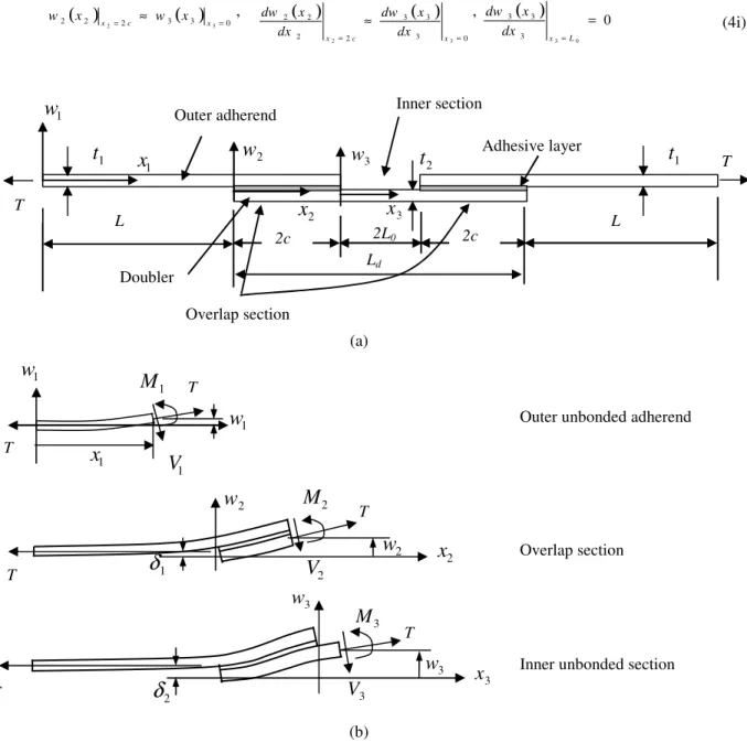
Theoretical analysis of joints is usually carried out using a simplified configuration without adhesive fillets at the overlap ends. Joint bending can be analyzed using beam theory, as initially suggested by Goland and Reissner in 1944.6 As shown in Figure 2, a butt joint has three sections; an outer unbonded adherend in section 1, a bonded overlap section in section 2, and an inner unbonded doubler part in section 3. In the following analysis, the joint deflection and bending stiffness in each joint section can be distinguished by its subscript. For instance, Di is the bending stiffness in the section ( 1 to 3). Note however that E1, E2, t1, and t2 refer to the Young’s modulus and thickness in the adherend (subscript 1) and the doubler (subscript 2). Deflections in the unbonded adherend, overlap section, and inner doubler section for the butt joint9, 18 are given by Eqns. (4a) to 4(c) with the origin of the coordinate frame located at the left side of each section’s centroid position.

( 1 1) 1 ( 1 1) 1 1 A cosh x B sinh x w = µ + µ (0 ≤ x1 ≤ L) (4a) ( 2 2) 2 ( 2 2) 1 2 2 = A cosh µ x + B sinh µ x +δ w (0 ≤ x2 ≤ 2c ) (4b)

(

3 3

)

3

(

3 3

)

2 3 3 = A cosh µ x + B sinh µ x +δ w (0 ≤ x3 ≤ L0) (4c)

where µi (i = 1 to 3) is given by Eq. (4d), Aiand Bi ( =i 1 to 3) are the integral constants and xiis the joint longitudinal position in section measured from the origin using its coordination system (Figure 2). The bending stiffnesses D1, D2, and D3 are given by Eqns. (4e), (4f), and (4g), respectively.

i i D T = µ (i = 1 to 3) _(4d)

(

k

)

adherend D 22 1 1

= (outer adherend section) _(4e)

(

)

2 1 2 2 2 3 2 1 1 1 1 2 ≈ D + E tδ + D + E t δ −δ D (overlap section) (4f)

(

k

)

doubler D 22 3 1

= (doubler within the inner gap section) _(4g) For aircraft structures, the adhesive thickness is very small and should generally be within 0.12 to 0.39 mm as suggested by MIL-17-V3-Ch6-Joints. The Young’s modulus of the adhesive is also much less than that of the laminated adherend and doubler. Thus, the adhesive can be treated as a sort of “spacer” in the overlap bending stiffness calculation (Eq. (4f)), having little other effect on the overall stiffness. The following six displacement boundary conditions are then applied:

( )

0 0 1 1 1= = x x w ,

_{( )}

_{( )}

0 2 2 1 1 2 1=L ≈ x = x w x x w ,

( )

(

)

0 2 2 2 1 1 1 2 1= = ≈ x L x dx x dw dx x dw (4h)

( )

2 2 3

( )

3 ₀ 2 x x₂= c ≈ w x x₃= w ,

(

)

( )

0 3 3 3 2 2 2 2 3 2= = ≈ x c x dx x dw dx x dw ,

( )

0 0 3 3 3 3 ₌ = L x dx x dw (4i) (a)

Outer unbonded adherend

Overlap section

Inner unbonded section

(b)

Figure 2. Schematic diagram of a general bonded composite butt joint configuration (a) and its bending deformation (b) when the joint in tension (not to scale).

The corresponding integration constants then become: 0 1 = A (4j)

(

)

(

)

(

)

( ) ( )

(

)

(

)

(

(

)

(

)

(

)

(

( ) ( )

)

)

2 2 1 1 1 2 2 0 3 1 3 1 3 1 2 2 tanh tanh 0 3 3 2 1 1 1 2 2 cosh tanh 0 3 2 1 1 tanh 2 tanh tanh 1 cosh tanh 2 tanh µ µ µ µ µ µ µ µ µ µ µ µ µ µ µ µ µ µ µ δ δ µ µ δ c L c L L c L L L c B + + + − + + = (4k)

(

)

(

)

(

)

( ) ( )

(

(

)

(

)

)

(

)

(

)

(

)

(

( ) ( )

)

2 2 1 1 1 2 2 3 2 1 2 1 3 2 tanh tanh 0 3 3 2 1 0 3 2 1 2 cosh 0 3 1 1 1 1 2 tanh 2 tanh tanh 1 tanh 2 tanh 1 tanh tanh sinh µ µ µ µ µ µ µ µ µ δ δ µ µ µ µ µ µ µ µ δ µ µ δ µ c _{L c} L c L L c L L L B A + + + + − = − = − (4l) 2

x

2

w

1

δ

w

2 2

M

T 2

V

T 3

V

3

w

3

x

2

δ

3

w

3

M

T T 3

x

Ld 2L0 1

w

T 2

x

1

t

1

x

w

2 2

t

t

1 3

w

L 2c 2c L Outer adherend Overlap section Inner section T Adhesive layer Doubler 1

x

1

w

1

M

1

w

1

V

T T

(

)

(

)

( ) ( )

(

(

)

(

)

)

(

)

(

)

(

)

(

( ) ( )

)

2 2 1 1 1 2 2 3 2 1 2 1 3 2 tanh tanh 0 3 3 2 1 0 3 2 1 2 cosh 0 3 1 1 2 1 2 tanh 2 tanh tanh 1 tanh 2 tanh tanh cosh µ µ µ µ µ µ µ µ µ δ δ µ µ µ µ µ µ µ µ δ µ µ µ µ c L c L c L L c L L B B + + + + + = = − (4m)

(

2

)

2

(

2

)

1 2 2 3=A cosh 2

µ

c +B sinh 2

µ

c +

δ

−

δ

A (4n)

(

3 0

)

3 3 A tanh L B =−

µ

(4o)

where δ1 is the transverse (vertical) distance between the neutral planes of the adherend (outer length of L) and bonded overlap section (overlap length of 2 in one adherend side); δ2 is the transverse distance between the neutral planes of the adherend and doubler (inner gap section length of 2L0) in the overlap section; the adherend thickness is

t1; and the doubler thickness is t2 (Figure 2). Thus, δ1 and δ2 can be expressed in Eqns. (4p) and (4q) as:

(

)

(

)

+ + + = + + + = adherend doubler k k t t t E t E t t 11 11 2 1 2 ' 2 1 ' 1 2 1 1 1 2 2 1 2 2η η δ (4p) 2 2 2 1 2 η δ = t +t + (4q)

where η is the adhesive thickness. The bending moments in the unbonded outer adherend, bonded overlap, and the inner doubler sections can then be expressed as:

(

1 1

)

1 2 1 1 2 1 1 TB sinh x dx w d D M = = µ (4r) ( ) ( ) ( 2 2 2 2 2 2 ) 2 T A cos x B sinh x M = µ + µ (4s)

(

)

(

)

(

3 3 3 3 3 3

)

2 3 3 2 3 3 T A cosh x B sinh x dx w d D M = = µ + µ (4t)

where T is the joint unit width tensile load.

2. Joint Elongation and Longitudinal Strain

When the joint is in tension, theoretical analysis of its axial elongation should be carried out under a plane stress condition. Ignoring out-of-plane deflection, the total joint elongation consists of four components arising from: (i) the outer adherends; (ii) the bonded overlap section; (iii) the adhesive shear between the doubler and adherend within the overlap section; and (iv) the inner central unbounded (not overlapped) doubler gap section.

The joint elongation can be approximated using the following expression: 3 2 1 2 2 l cG T l l l a ∆ + + ∆ + ∆ = ∆ η _(5a)

where = adhesive shear modulus, = adhesive thickness, = half bonded length in one adherend side, = the joint tensile load, and

1 1 1 t E L T l =

∆ (elongation in one outer unbonded adherend) (5b)

overlap overlap t E c T l₂ = 2

∆ (elongation in the one side overlap section) _(5c)

a

G c

T

η

(effect of adhesive shear) _(5d)

doubler doubler t E L T l3 0 2 =

∆ (elongation in the inner unoverlapped doubler section) (5e) For the current elongation estimation, the value of the outer unbonded adherend length, L = 69.2 mm, was used. This length was measured from the tab edge of the gripped part to the adherend bonded overlap edge, as shown in Figure 1. Since the stiffnesses of both the adhesive fillets and the tapered tabs are very low, their contributions to the overall joint stiffness can safely be ignored.

Longitudinal strain on the joint surface consists of both axial tensile strain and bending strain. Theoretical analysis of axial strain should be carried out using an in-plane condition. According to Eqns. (1a) to (1c), the resultant strain at the laminate surface position can be determined as:

2 2 11 22 22 11 t M k T k t M k N k x x x = ± = ±

ε

(5f)

where the tensile “+” or compressive “−” sign is determined by the bending condition at that specific location.

3. Adhesive Stresses in the Composite Butt Joints

Basic parameter in the adhesive stress equations

A single-strap butt joint is fabricated using two single-lap joints. The coupled adhesive stress differential equations for a butt joint are identical to that of a single-lap joint, except for the boundary conditions consisting of the bending moment and shear force at the overlap ends. Through equilibrium analysis in the bonded overlap section, the adhesive stress equations can be derived as:6, 18, 19

0 2 1 3 3 = + + a a a a dx d a dx d

σ

τ

τ

(6a) 0 2 1 4 4 = + + dx d b b dx d _a a a

_σ

τ

σ

(6b) where a1, a2, b1, and b2, are four basic parameters which have to be determined prior to the exploration of the adhesive peel and shear stresses, and . Among the four parameters, a2 and b2 are coupling parameters between the adhesive peel and shear stresses. These coupling parameters vanish when dealing with identical materials having the same thickness for the adherends and doubler.

For a composite butt joint fabricated using different adherend and doubler laminates, the four parameters can be determined as: + + − + + −

≈ ₋adherend ₋doubler ₋adherend ₋doubler ₋adherend ₋doubler

a _{k k tk t k} t _k t _k G a 22 2 2 22 2 1 12 2 12 1 11 11 1 4 4

η

(6c)

−

+

+

=

−adherend −doubler −adherend −doubler a

k

t

k

t

k

k

G

a

2 ₂₂ 22 1 12 12 2

2

2

η

(6d)

(

adherend doubler

)

a k k E b1 = 22− + 22− η (6e) − + + −

≈ −adherend −doubler −adherend −doubler

a _{k k} t _k t _k E b 2 ₂₂ 22 1 12 12 2 2 2 η (6f)

The equations relating the adhesive stress to the joint deformation are given in Eqns. (6g) and (6h):6,7, 10, 18, 19

η σ u d a a w w E − = (6g) η τ u d a a u u G − = (6h)

where Ea and Ga are adhesive Young’s and shear moduli; wu and wd are deflections in the adherend and doubler and

uu and ud are displacements at the adherend-adhesive and adhesive-doubler interfaces.

Under a plane strain condition, the four parameters of a1, a2, b1, and b2 can be determined using the corresponding kij terms given in Eqns. (2b) to (2e).

First strategy for exploring adhesive stresses

The uncoupled equation for the adhesive shear stress can be obtained by eliminating the peel stress in Eq. (6a) as:

(

1 1 2 2

)

0 3 3 1 5 5 1 7 7 = − + + + dx d b a b a dx d b dx d a dx d τ_a τ_a τ_a τ_a (7a) The corresponding characteristic equation becomes:10, 18, 21-23

(

)

(

1 1 2 2

)

0 2 1 4 1 6 _{+ a λ + b λ + a b − a b =} λ λ (7b)

Once the seven roots are determined, the general solution for the adhesive stress can be established and its seven constant integrals can be identified using the following seven boundary conditions:18

T dx c c a = − −

τ

(7c) + + + = − − − − − = 0 12 1 12 12 1 11 2 2 k M t k T k t k G dx d adherend adherend adherend adherend a c x a η τ (7d) + − + + − = − − − − = 1 12 2 12 12 2 11 2 2 k M t k T k t k G dx d doubler doubler doubler doubler a c x a η τ (7e)

0 22 1 12 1 2 2 2k V t k G a dx d adherend adherend a c x a a _{+ = +} − − − = η τ τ (7f) 1 22 2 12 1 2 2 2k V t k G a dx d doubler doubler a c x a a _{+ = − +} − − =

η

τ

τ

(7g)

(

12 22 0

)

2 3 3 1 5 5 M k T k E a dx d a dx d adherend adherend a c x a a − − − = + − = + η τ τ (7h)

(

12 22 1

)

2 3 3 1 5 5 M k T k E a dx d a dx d doubler doubler a c x a a − − = + = + η τ τ (7i) The general solution of the adhesive peel stress can then be explored using its fundamental equation:

dx d b b dx d _a a a _σ τ σ 2 1 4 4 − = + (7j)

This nonhomogeneous equation can be investigated using Variation of Constants or Lagrange’s method. 22, 23 The general solution is established by combining the general solution of its homogeneous equation and any one particular solution of its nonhomogeneous equation. A detailed derivation of adhesive stresses in a bonded isotropic butt joint was presented by Li,18 where the general adhesive stress solutions were determined and good agreement was shown between closed-form solutions and finite element predictions.

Second strategy for exploring adhesive stresses

The uncoupled sixth order differential equation for adhesive peel stress can be derived by eliminating adhesive shear stress in Eq. (6b) as:19

( 1 1 2 2) 0 2 2 1 4 4 1 6 6 = − + + + a a a a _{a b a b} dx d b dx d a dx d σ σ σ σ (7k) Note from the two uncoupled adhesive stress differential equations in Eqns. (7a) and (7k), that their characteristic equations would have up to six common roots, λi (

i

=

1 to 6). One more characteristic root of

0

=

λ

exists for the adhesive shear stress. The expression for the general solution of the adhesive shear stress will have seven terms, and the expression for the general solution for the peel stress will have six terms. These six terms are identical to the adhesive shear stress expression and are determined by the characteristic roots.

The same procedure used to explore the adhesive shear stress solution in strategy one can be used in strategy two. The seven boundary conditions were presented in reference.19

Two different boundary conditions exist between the two sets of boundary conditions (Eqns. (7c) to (7i), and the second set of boundary conditions in reference19). The last two boundary conditions in reference19 were replaced by the fourth and fifth conditions (Eqns. (7f) and (7g)) in the first set of boundary conditions.18 The six integral constants in the general peel stress solution expression can then be determined using the following boundary conditions: 0 V V V dx u x c u _{x c} c c a = =− − = = −σ (7l)

(

V0c M0

)

dx x c c a =− + − σ (7m)

(

12 22 0

)

2 2 M k T k E dx d adherend adherend a c x a − − − = + = η σ (7n)

(

12 22 1

)

2 2 M k T k E dx d doubler doubler a c x a − − = + − = η σ (7o) 0 22 2 3 3 V k E b dx d adherend a c x a a − − = = +

η

τ

σ

(7p) 1 22 2 3 3 V k E b dx d doubler a c x a a − = − = + η τ σ (7q) The final closed-form solutions for adhesive shear and peel stresses were not provided by Bigwood and Crocombe.19 Furthermore, they did not provide the six boundary conditions needed to explore the peel stress. These two uncoupled differential equations derived by Bigwood and Crocombe could be used as a starting point for other researchers to carry out the development of closed-form solutions, which would avoid the complex derivations

and long expressions required for calculating peel stress using strategy one. Exploration of closed-form solutions will be carried out and presented in another paper. The first boundary condition set expressed in Eqns. (7c) to (7i) will be used for shear stress derivation for the bonded composite butt joints discussed herein. These boundary conditions led to good agreement between the closed-form solutions of the proposed strategy one and FE results for butt joints made of isotropic materials.18 Thus, the impact of the two different sets of boundary conditions on the adhesive shear stress will not be studied further.

IV. Geometrically Nonlinear Finite Element Simulations

A. Finite Element Modeling

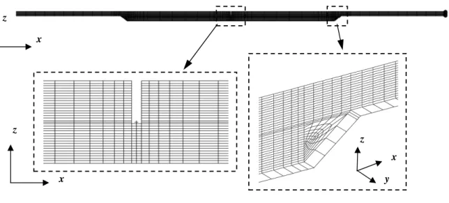
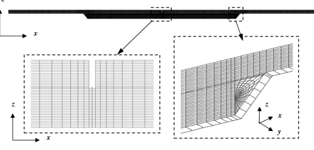
To properly set up the lamina orientation in each ply and achieve fast and accurate numerical analyses, three-dimensional finite element (FE) models of the experimental joints (with unit-width, i.e. 1 mm in the y-direction) were generated, using the MSC.Patran (pre- and post-processor) version 2008r2 and MSC.Marc (solver) version 2008. A total of 5,330 nodes and 2,536 8-node brick elements (2 wedge elements included) were used for the case 1 joint (Figure 3), and a total of 6,370 nodes and 3,054 8-node brick elements (2 wedge elements included) were used for the case 2 joint (Figure 4). The outer adherend length was 54.2 mm in the models. Joint deformation under a two-dimensional plane strain condition was analyzed by applying the zero displacement condition, Uy = 0, at the two joint side edges along the longitudinal x-direction. Joint width direction was in y-axis, and thickness was in the z-direction. One element was meshed along the joint unit width, as well as in each lamina thickness z-direction. Two elements were created along the adhesive thickness in the overlap section. A relatively fine mesh was created in the joint transition areas in the outer and inner overlap edge regions. Adhesive fillets were simply assumed to be a triangular prism at the outer overlap edges. A 0.5 mm inner gap between the two adherends, as well as the adhesive layer, was built in the models to reflect the actual joint configuration with an adhesive crack induced during the first tensile ramp.

In addition to the displacement condition of Uy = 0 at the joint’s two side edges, the following boundary conditions, were used during the joint tensile loading stage: (i) displacement of Ux = Uy =Uz = 0 set at the joint left remote adherend edge; (ii) displacement of Uz = 0 applied to the two middle nodes at the right remote adherend edge; (iii) multi-point constraint (MPC) condition applied to the nodes at the right remote edges ensuring the same longitudinal displacement (Ux); (iv) uniform tensile stress applied to the joint right adherend edge; and (v) geometrically nonlinear FE analysis. FEA results for each pair of nodes, located at the [x, 0, z] and [x, 1, z] positions on the two width side surfaces, were almost identical.

Figure 3. Three-dimensional finite element model for the case 1 joint using a total of 5,330 nodes and 2,536 8-node brick elements (2 wedge elements included).

x z x z x z y

Figure 4. A total of 6,370 nodes and 3,054 8-node brick elements (2 wedge elements included) were created in the three-dimensional finite element model for the case 2 joint (thicker doubler).

V. Results and Discussion

The adhesive bond within the joint middle inner gap cracked at a tensile load of approximately 4.5 kN (177 N/mm, per-unit-width) during the first load cycle to peak load (i.e. 5.5 kN). The onset of cracking could be detected audibly as well as through a discontinuity in the measured strain curves. Strain and displacement (elongation) data from the two subsequent load cycles were used to study joint deformation. Little difference in the elongation and strains between the two types of joints was found. Average data obtained from the two tests for each joint case 1 and joint case 2 were used in the following studies of the joint elongation and strain.

A. Out-of-Plane Deflection of the Joint

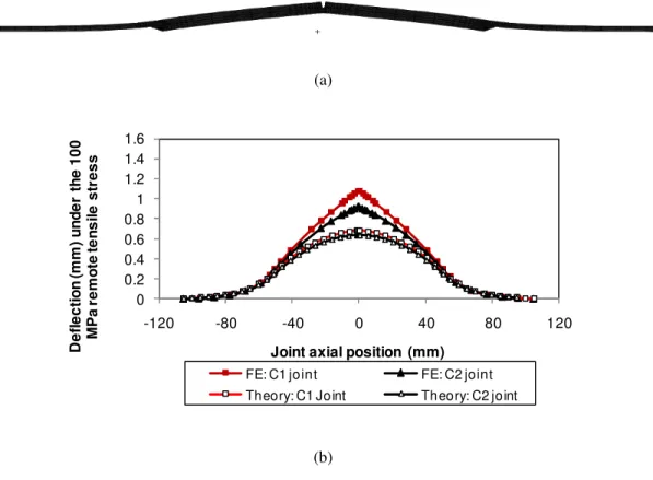
Out-of-plane deflections arise when the butt joint is in tension. Figure 5 shows joint deflections under a 100 MPa remote tensile stress, obtained from finite element and theoretical results. Peak deflection occurred in the joint middle region, with a maximum magnitude of approximately 1 mm, a very small value compared to the joint overall length of the approximate 210 mm. Peak deflections were Uz = 1.08 mm (case 1 joint by FE), 0.90 mm (case 2 joint by FE), 0.69 mm (case 1 joint by theory under a plane strain condition), and 0.62 mm (case 2 joint by theory under a plane strain condition). The relative difference between theory and FE predictions was approximately 36% for the case 1 joint and 31% for the case 2 joint. This difference was mainly the result of the displacement continuity conditions constrained at the overlap edges, presented in Eqns. (4h) and (4i), in the theoretical derivation. At the two outer overlap edges, (x = ± 50.8 mm positions if x = 0 is at the joint middle position), there was limited difference between the FE and theoretical results. Finite element results are more accurate than theoretical predictions, since approximate displacement boundary conditions were used at the joint transition edges in the theoretical derivations. It can be seen from Figure 5 that: (i) the theoretical model underestimated the deflection at the inner overlap edge region; and (ii) the deflection difference was lower for the thicker doubler. As a result, the bending moment would be overestimated at the inner overlap edge and underestimated at the middle position of inner gap region. The impact of these shortfalls on the joint strain could be partially discerned in the subsequent strain comparisons. In general, the theoretical model was found to correlate well with the finite element results within the applied load range.

x z x z x z y

(a)

(b)

Figure 5. Illustration of secondary bending in a bonded butt joint (a) and comparison of joint deflection predictions from the FE model and the theoretical model for 100 MPa remote tensile stress (b).

B. Joint Elongation

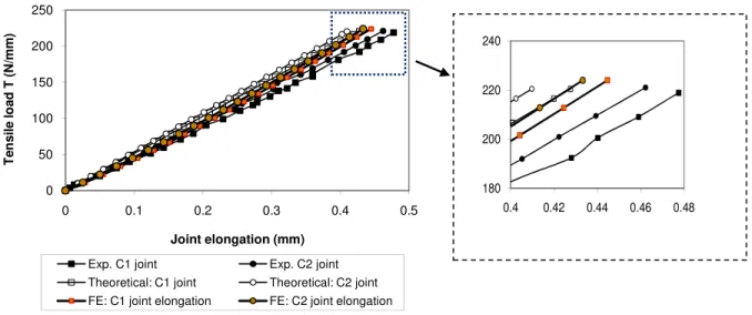
Joint elongation versus tensile load is shown in Figure 6. A linear variation was observed, and good agreement was found between experimental, theoretical, and finite element results. Theoretical joint elongation results were obtained using Eq. (5a). As stated earlier, identical laminated adherends were used in both joint cases. The only difference between the two was the doubler, which for the case 2 joint was 50% thicker than the case 1 joint (for the case 1 joint, the doubler was identical to the adherends). At the peak tensile force of 220 N/mm, theoretically predicted joint elongations were approximately 90% and 89% of the measured values for the case 1 and case 2 joints respectively with the finite element results falling between measured and theoretical values. The over-prediction of joint stiffness may be the result of several factors: (i) inaccuracy in the elongation estimated for the overlap section and its transition area; (ii) differences between the effective laminate Young’s moduli used in the theoretical model and the finite element models, and those in the actual tests; (iii) possible slip between the grips and the joint end tabs; (iv) impact of adhesive shear deformation between the end tab and joint adherend; and (v) differences in the dimensions between the designed and manufactured/tested joints, etc. Despite these factors the theoretical model correlates quite well with the experimental and finite element results.

0 0.2 0.4 0.6 0.8 1 1.2 1.4 1.6 -120 -80 -40 0 40 80 120 D e fl e c ti o n ( m m ) u n d e r th e 1 0 0 M P a r e m o te t e n s il e s tr e s s

Joint axial position (mm)

FE: C1 joint FE: C2 joint

Theory: C1 Joint Theory: C2 joint

Figure 6. Comparison of the joint elongation during the tensile loading stage obtained from the experimental tests and theoretical estimations.

C. Strain Variation at the Longitudinal Strain Gauges

1. Effect of the Plane Strain and Plane Stress Conditions on the Axial Strains

Joint strain measurements could be used to determine if it is more appropriate for the theoretical model to use plane strain or plane stress assumptions. Axial strain in the inner gap section can be easily estimated using either the measured strain from gauges 2 and 3 at the outer adherend or strain results (

ε

_x0) from the theoretical analysis (Eqns. (2e), (3a), and (3b)). For the case 1 joint, the axial strain in the inner gap section should be the same as that for the outer adherend. For the case 2 joint, the axial strain in the inner gap section should be t1 t2 ≈ 0.67 of the

outer adherend axial strain, due to the 50% thicker doubler.

Since strain gauge 1 measured the resultant strain from deformation in three areas including the overlap end regions, this gauge could not be used to estimate axial strain for the inner section. The average of the strains measured by gauges 2 and 3 were used to determine the axial strain of the outer adherend using:

2 3 2 G G axial ε ε ε = + (8a)

The corresponding axial strain was theoretically estimated using:

1 ' 1t E T axial = ε _(8b)

where T, t1, and E are joint tensile load (per unit-width), adherend thickness, and the effective Young’s modulus 1'

of the adherend laminate, respectively. ' 1

E is E1under the plane stress condition, and

' 1

E becomes E₁

(

1−v₁₂v₂₁

)

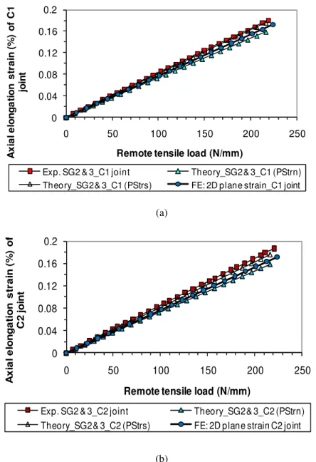
under plane strain conditions.12 Figure 7 shows the axial strain variation in the outer adherend obtained from experimental, theoretical, and finite element results. For the two joint cases, axial strains in the outer adherend should be the same since they use identical adherends. In both cases, the best agreement was achieved between the experimental data and theoretical results under an assumed plane stress condition. In particularly, experimental data in the case 1 joint was virtually identical to the theoretical results. The theoretically predicted strains under plane strain conditions were approximately 8% lower for case 1 joint and 10% for the case 2 joint. The finite element results were between the theoretical results under plane stress and strain conditions. This suggests that a plane stress condition provides a closer estimation of joint axial strains and validated the later use of a plane stress condition for joint elongation analysis. As predicted, the stiffer doubler of the case 2 joint did not significantly affect the

0 50 100 150 200 250 0 0.1 0.2 0.3 0.4 0.5 T e n s il e l o a d T ( N /m m ) Joint elongation (mm)

Exp. C1 joint Exp. C2 joint

Theoretical: C1 joint Theoretical: C2 joint

FE: C1 joint elongation FE: C2 joint elongation

180 200 220 240

0.4 0.42 0.44 0.46 0.48

longitudinal strain in the adherends. Two samples for each joint case were tested with a measured difference of no greater than 2.5% for any strain reading.

(a)

(b)

Figure 7. Comparison of experimental and theoretical adherend axial strains at the strain gauge 2 and 3 positions for the case 1 (a) and case 2 (b) joints. In these labels, “PStrn” and “PStrs” refer to the plane strain and plane stress conditions, “SG” refers to strain gauge, and “C1 jt” or “C2 jt” refer to case 1 or case 2 joints.

2. Approach for Establishing Strain Continuity within the Gauge Length of Strain Gauge 1 in Theoretical Analysis

Strain gauges 2 and 3 had an effective gauge length of approximately 1.58 mm, which spanned only one section on the adherend, well away from the overlap ends. Thus, constant strain within the gauge length could be assumed. Theoretical estimations for these strains can be obtained using Eq. (5f).

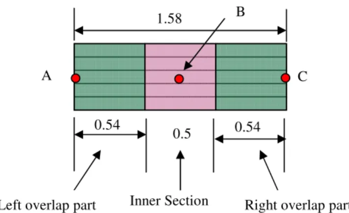
On the other hand, strain gauge 1 spanned three different sections, as shown in Figures 1 and 8(a): a 0.54 mm length on the left side overlap section; a 0.5 mm length on the inner gap section; and a 0.54 mm length on the right side overlap section. Since the strain variation along the doubler outer surface should be continuous, an approach is

0 0.04 0.08 0.12 0.16 0.2 0 50 100 150 200 250 A x ia l e lo n g a ti o n s tr a in ( % ) o f C 1 jo in t

Remote tensile load (N/mm)

Exp. SG2 & 3_C1 joint Theory_SG2 & 3_C1 (PStrn)

Theory_SG2 & 3_C1 (PStrs) FE: 2D plane strain_C1 joint

0 0.04 0.08 0.12 0.16 0.2 0 50 100 150 200 250 A x ia l e lo n g a ti o n s tr a in ( % ) o f C 2 jo in t

Remote tensile load (N/mm)

Exp. SG2 & 3_C2 joint Theory_SG2 & 3_C2 (PStrn) Theory_SG2 & 3_C2 (PStrs) FE: 2D plane strain C2 joint

proposed here to ensure strain continuity and to estimate the corresponding average strain. This approach aims to provide a useful application of the theoretical analysis method, as well as to provide an explanation of the obtained experimental data. The left and right side overlap sections had the same deformation and strain variation. Since there could be little strain variation within each of the three small sections, a constant distribution was assumed to exist in each section. Three points A, B, and C were chosen at the left edge, centre, and right edge of the strain gauge, such that they were away from the overlap end. The strain at point A was the same as the strain at point C. According to the mode of joint deformation, the strain at point B was compressive with a strain magnitude greater than at points A and C. Strains at these points, estimated using Eq. (5f), were assumed to be constant throughout each section. As shown in Figure 8(b) and (c), two different strain discontinuity scenarios could be encountered through application of a tensile load to the joints; these can be dealt with using the following approaches:

Strain situation 1, as shown in Figure 8(b)

When the strain ε_A at both points A and C was positive (in tension) and the strain ε_B at point B was in compression, the assumed linear strain variation is shown in the right side of Figure 8(b). The algebraic sum in these positive and negative areas was computed and the average strain was determined by a direct summation of the strain areas and dividing by the 1.58 mm gauge length.

Strain situation 2, as shown in Figure 8(c)

When the strains at points A (or C) and B were negative (in compression), the assumed linear strain variation is shown in the right side of Figure 8(c). The average strain was again computed by summing the strain areas and dividing over the 1.58 mm gauge length.

The two situations can be easily identified during tensile loading. An Excel spreadsheet was then used to compute the corresponding average strain for comparison with the experimental data.

3. Strain Comparison

Longitudinal strain was calculated under both plane strain and plane stress conditions. This was accomplished using Eq. (5f) with the appropriate Young’s modulus and bending stiffness. The joint bending moments (second term in Eq. (5f)) can be calculated using Eqns. (4r) to (4t) for specific locations. The related six integral constants (Eqns. (4j) to (4o)) can be determined using the corresponding joint geometric data (L = 54.2 mm,

c

= 50.675mm,

L0 = 0.25 mm, etc.) and remote tensile load. If a value of L = 74.2 mm is used, the calculated bending moments are almost identical to those ones obtained using a value of 54.2 mm, since the effect of the adherend length on the bending moment variation can be eliminated for joints when L c >2.10

Finite element results were taken from the nodes corresponding to strain gauges 2 and 3, while average strain from the nodes located within the strain gauge region was used to represent the strain gauge 1 value due to the large local strain variations.

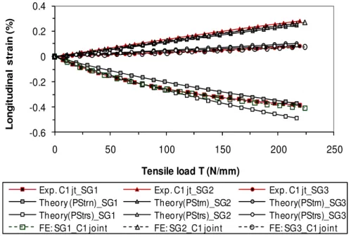
Figure 9 shows the strains obtained from the three methods for the case 1 (a) and case 2 (b) joints. This strain consisted of the axial strain component under a plane stress condition and the strain induced by bending. Good agreement was achieved among experimental, theoretical, and finite element results in both joints, especially for the case 1 joint. In both casea, finite element results were virtually identical to experimental data for the three strain gauges. Similar strain variations were observed in the two joint cases with compressive strain occurring at strain gauge 1 and tensile strains occurring at strain gauges 2 and 3. The stiffer doubler in the case 2 joint led to markedly smaller strains in the inner section (strain gauge 1) than in the case 1 joint, which also affected the strains at the outer adherends. The measured strains at strain gauges 1, 2 and 3 in the case 1 joint were approximately 135%, 92%, and 118% respectively, higher than the corresponding strains in the case 2 joint. Additional details regarding each strain gauge response are given below.

Strain gauge 1

For the case 1 joint (Figure 9(a)) the measured strains and finite element results were between the strains estimated assuming plane strain and plane stress conditions, with strains predicted using a plane stress condition being slightly greater than those predicted using a plane strain condition. The strain difference between these two predictions was approximately 0.11% at peak load (220 N/mm tensile load). For a tensile load from 0 to 100 N/mm, the measured strains could be accurately predicted using a plane stress assumption; for tensile loads between 100 and 175 N/mm, the measured strains were between those calculated using plane strain and plane stress conditions; for a tensile load between 175 to 220 N/mm, the measured strains compared better with those estimated using a plane strain assumption.

For the case 2 joint (Figure 9(b)) the measured strain gauge 1 strains were best represented assuming a plane stress condition during the entire tensile loading ramp. The finite element results were virtually identical to the measured data. The difference between these two predictions (plane stress and plane strain) was less than that of

case 1 joint with a maximum difference of 0.066% at the highest tensile load of 220 N/mm. The excellent agreement between the experimental, FE, and theoretical results for strain gauge 1 demonstrated that the approach proposed for ensuring strain continuity and for estimating the average strain is acceptable as a practical engineering solution.

Strain gauges 2 and 3

The maximum strain difference between the plane stress and plane strain conditions at each strain gauge location was approximately 0.013% at the 220 N/mm tensile load for both joints, much less than the differences in strain gauge 1. This strain difference may be affected by the degree of bending in the joint with the larger the degree of bending, the greater the strain difference.

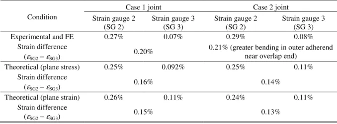
The theoretical predictions matched the experimental results for both the case 1 and case 2 joints. Table 1 gives both experimental and theoretical strains when these joints are loaded at the maximum tensile load of 220 N/mm. From the measured strain data (εSG2 − εSG3), it can be seen that the degree of outer adherend bending was slightly

greater in the case 2 joint than in the case 1 joint. This difference could not be clearly seen in the theoretical calculations.

Table 1. Strains in strain gauges 2 and 3 obtained from experimental measurement and theoretical analysis at a tensile load of 220N/mm (unit width) referring to Figure 9.

Condition

Case 1 joint Case 2 joint

Strain gauge 2 (SG 2) Strain gauge 3 (SG 3) Strain gauge 2 (SG 2) Strain gauge 3 (SG 3) Experimental and FE 0.27% 0.07% 0.29% 0.08% Strain difference (εSG2 − εSG3)

0.20% 0.21% (greater bending in outer adherend near overlap end)

Theoretical (plane stress) 0.25% 0.092% 0.25% 0.11% Strain difference

(εSG2 − εSG3)

0.16% 0.14%

Theoretical (plane strain) 0.26% 0.11% 0.24% 0.11%

Strain difference (εSG2 − εSG3)

0.15% 0.13%

The discrepancy in the strain comparisons between the experimental, finite element, and theoretical predictions could be explained by the following: (i) differences between the averaging approach used in the theoretical calculations and the actual measured strain gauge values; (ii) differences in the actual and modelled material properties; (iii) inaccuracies in the idealized joint condition used in the theoretical analysis, for example, adhesive fillets at the overlap ends and the joint tapered tabs were not included, etc.24 In general, good agreement in strains between the theoretical, finite element, and the experimental results was achieved, demonstrating that the proposed approach for ensuring strain continuity in the overlap end region can be used for practical applications, and the theoretical methods for the strain analysis are not affected as significantly as the deflection prediction.

(a) Three regions covered by the 1.58 mm gauge length of strain gauge 1

(b) Strain situation 1 and its continuity approach

(c) Strain situation 2 and its continuity approach

Figure 8. Schematic of the approximate approach used to ensure strain continuity within the gauge length of strain gauge 1 for two different strain distribution scenarios (dimensions in mm).

B C A 0.5 1.58 0.54 0.54 Inner Section

Left overlap part Right overlap part

0.54 0.54 A

ε

+ + + + − − − − 0.5 B

ε

A

ε

B

ε

0.54 0.54 0.5

−

+

+

+

+

+

+

+

+

0.54 0.54 B

ε

0.54 _0.5 0.54 − − − − −− −− A

ε

_ε

_A B

ε

− − − − − − − − 0.5 − − − −

(a) Case 1 joint (C1 jt) using identical laminates

(b) Case 2 joint (C2 jt) with thicker doubler

Figure 9. Comparisons of longitudinal strains of strain gauges 1 to 3 for the two joint cases obtained from experimental measurements and theoretical calculations.

-0.6 -0.4 -0.2 0 0.2 0.4 0 50 100 150 200 250 L o n g it u d in a l s tr a in ( % ) Tensile load T (N/mm)

Exp. C1 jt_SG1 Exp. C1 jt_SG2 Exp. C1 jt_SG3

Theory (PStrn)_SG1 Theory(PStrn)_SG2 Theory(PStrn)_SG3 Theory(PStrs)_SG1 Theory(PStrs)_SG2 Theory(PStrs)_SG3 FE: SG1_C1 joint FE: SG2_C1 joint FE: SG3_C1 joint

-0.6 -0.4 -0.2 0 0.2 0.4 0 50 100 150 200 250 L o n g it u d in a l s tr a in ( % ) Tensile Load T (N/mm)

Exp. C2 jt_SG1 Exp. C2 jt_SG2 Exp. C2 jt_SG3

Theory (PStrn)_SG1 Theory(PStrn)_SG2 Theory(PStrn)_SG3 Theory(PStrs)_SG1 Theory(PStrs)_SG2 Theory(PStrs)_SG3 FE: SG1_C2 joint FE: SG2_C2 joint FE: SG3_C2 joint

D. Adhesive Stress Profile along the Longitudinal Bondline

Derivation of a closed-form solution for adhesive stress would be a tedious job, even with several simplificaitons in joint configuration and material behaviour.18 For bonded composite butt joints with different adherend and doubler, no closed-form solutions were found in the open literature. Finite element results are used in this study. Figure 10 shows the adhesive peel stress profile with significant variation at the overlap edges, especially at the inner edge. Peak stress was located at the inner edge and was much greater than the outer edge value, due to the bending condition. The highly nonlinear region was approximately 10 mm in length in both the outer and inner overlap edge regions, with almost zero peel stress within the overlap middle section, as shown in this figure. The peak stress at the inner overlap edge was approximate 96 MPa for the case 1 joint and 80 MPa for the case 2 joint, a difference of about 17% for the thicker doubler. The stress magnitude at the outer overlap edge was effectively decreased by the presence of an adhesive fillet, compared with a non-fillet joint case.18 The maximum peel stress was calculated to be around 8 MPa in the case 1 joint and 10 MPa in the case 2 joint at the outer overlap fillet region.

Variation in the adhesive shear stress is shown in Figure 11, with a similar profile to the peel stress. The highly nonlinear stress distribution was similar to the peel stress and also occurred within approximate 10 mm of the outer and inner overlap edge regions. Again near zero shear stress was found within the overlap middle section. Peak stress was located at the inner edge and was much greater than the outer edge value at approximately 73 MPa for the case 1 joint and 60 MPa for the case 2 joint. The magnitude of the adhesive shear stress at the outer overlap edge was around 10 MPa for both joint cases. Numerical results suggested that the joint bonding strength would be mainly affected by adhesive stress at the inner edge region, and that proper attention and action should be taken in that area to ensure a sufficient margin of safety.

Figure 10. Adhesive peel stress, , variation along the bondline for the 100 MPa joint remote tensile stress

predicted by finite element analysis. -20 0 20 40 60 80 100 -60 -40 -20 0 20 40 60 A d h e s iv e p e e l s tr e s s ( M P a )

Longitudinal adhesive position (mm)

FE: C1 joint FE: C2 joint -20 0 20 40 60 80 100 -5 -3 -1 1 3 5 -5 0 5 10 45 47 49 51 53 55