A “big-data” algorithm for KNN-PLS
Maxime Metz 1,2, Matthieu Lesnoff 2,3,4, Florent Abdelghafour1,2, Reza Akbarinia5, Florent Masseglia5, Jean-Michel Roger 1,2
1ITAP, Univ Montpellier, INRAE, Institut Agro, Montpellier, France
2ChemHouse Research Group, Montpellier, France
3CIRAD, UMR SELMET, Montpellier, France
4SELMET, Univ Montpellier, CIRAD,INRA,Institut Agro, Montpellier,France
5
Inria & LIRMM, Univ Montpellier, France
Corresponding author
Maxime Metz
Email: [email protected]
Postal address: 361 Rue Jean François Breton, 34196 Montpellier
Keywords :
KNN-PLSDA, PLSDA, parSketch, Big-data, local-PLS
A well known issue regarding PLS lies in the difficulty to apprehend nonlinearities. As a solution, an extension of the method, “KNN-PLS”, was developed. However, this solution is based on a neighbourhood selection algorithm whose execution time is highly dependent on the size of the database, leading to prohibitive response times. This article proposes, as an alternative, a new method designed to process large data volumes: “parSketch-PLS”. This method combines a “big-data domain” neighbour selection method, called "parSketch", and the PLS method. Essentially, this paper presents a feasibility study, regarding the adaptation of big-data principles for spectral datasets, in non-linear contexts. The parSketch method has not been studied in the context of chemometrics and considering the specific properties of spectral data. This method is based on the approximation of sample neighbourhoods, based on spectral distances. It is then necessary to investigate the relevance of these neighbourhoods for PLS models and predictions. This article compares PLS and KNN-PLS methods with the parSketch-PLS method. In this context, PLS allows to process large volumes of data quickly but performs poorly in prediction while the KNN-PLS method returns accurate predictions, yet with much higher computational time. This paper shows that the proposed pairing offers a good operational trade-off between prediction performances and computational cost. In addition a comprehensive study of the input parameters of parSketch-PLS is conducted. The objective is to understand the influence of these parameters on the prediction performances. This article proposes a framework to interpret the neighbourhoods returned by comparing their relative sizes with the evolution of performances and the input parameters of parSketch.
1. Introduction
Chemometrics exploits a wide range of tools for the analysis and interpretation of spectroscopic data. One of the objectives of these tools is to associate spectral information with physicochemical properties in order to predict these properties. Among them, a reference method is PLSR (Partial Least Squares Regression) [1]. It is a relevant method in various
fields such as bioinformatics and social sciences. PLSR enables to realise very efficient predictive models when there is a linear relationship between the spectra and the physicochemical property(ies) of interest. PLSR is composed of a dimension reduction step (PLS) followed by a regression on the scores produced. Similarly, it is possible to carry out a discrimination calculating a discrimination model on the PLS scores. This article focuses on the two methods, under the term PLS. Due to the diversity of applications in the field, it is common to be confronted with data resulting from the aggregation of measurements carried out on samples of different natures. This aggregation often introduces non-linearities in the data (curvatures, clustering). These nonlinearities can significantly alter the quality of the predictions[2]–[4]
. A solution to this problem is the use of "local" methods
[2], [5]–[10]. One of the most common local methods is "KNN-PLS" (K Nearest Neighbours - PLS) [2], [5], [9], [11]–[19]. The KNN-PLS method consists in determining a neighbourhood of the sample to be predicted, using a similarity criterion, and then calculating a PLS model on the neighbourhood of this sample. This method solves regression problems by computing a PLSR model on each neighbourhood. This method can also be applied to classification problems by computing a PLSDA (PLS Discriminant Analysis) model [20] on the neighbourhood. Similarity criteria is one of the most studied issues regarding implementations of KNN-PLS models [21], [22]. However, paradoxically, only a few studies have been conducted on neighbours selection and on the associated algorithms. Current KNN-PLS methods are all implementations of the “brute-force” algorithm, which consists in calculating all dissimilarities between the sample to be predicted and all the samples in the database, then ordering these samples according to the dissimilarities. The "brute-force" algorithm has the advantage of being a straightforward and accurate calculus. However, it is fastidious or even unfeasible to process large databases using this method.
Recent developments in spectroscopic instrumentation (especially hyperspectral imaging) make it possible to acquire large volumes of data. It becomes then unreasonable to apply methods as computationally intensive as the "brute-force" algorithm on these data. An
alternative is the use of "big-data" methods. Numerous methods have been developed in this field in order to accelerate the search for neighbours. All these methods share the central notion of indexation [23]–[27]. An index is a data structure that enables the search for samples in a time that is sub-linear (often logarithmic) to the size of the database. Therefore, indexing a database consists in adding its data to the index structure to be able to find them quickly. However, the conventional indexing structures are not suitable for spectral data, as they contain large numbers of highly inter-correlated variables. Recently, indexing methods have been developed to deal with time series [28]–[35] which present similar issues with spectral data. However, only a few time series indexing methods are suitable for large volumes of data. Two methods have recently been developed to be processed with extensively parallel architectures in order to process quickly large databases: DPiSAX (Distributed Partitioned indexed Symbolic Aggregate approXimation) [36]and parSketch[37], [38].
In chemometrics, these algorithms have not been tested yet and would solve some major methodological issues, such as finding a fast and reliable neighbour search in the KNN-PLS framework. In this work, it is proposed to study parSketch in the context of chemometrics in order to evaluate the potential of this method to realise applications in chemometrics. The parSketch method combines dimension reduction, achieved by projection on random vectors
[37] , with the creation of lists of samples based on grids. ParSketch’s efficiency has been
illustrated in terms of calculation cost compared to the "brute-force" method[37], [38].
In this paper, it is proposed to conduct a feasibility study of the parSketch method on spectral data. For that, parSketch has been evaluated to replace the "brute-force" algorithm in the KNN-PLS method, i.e. to use the parSketch method and then compute a PLS model on the resulting neighbourhood ("parSketch-PLS"). However, parSketch approximates a
neighbourhood. It is therefore necessary to test the influence of this approximation on the quality of PLS results.
2. Theory
2.1.
Notations
Capital bold characters will be used to designate matrices, e.g. X ; small bold characters for column vectors, e.g. xj will denote the j th column of X; row vectors will be denoted by the transpose notation, e.g. xTi will denote the i th row of X; non bold italic characters will be used for scalars, e.g. matrix elements xij or indices i.
2.2.
Method description
The creation of an index with parSketch is done in two steps: dimension reduction and grid creation [37], [38]. Let X(np) be the matrix of n spectra per p wavelengths. Let P(pv) be a matrix
of v vectors of dimension p, containing the values -1 or 1 according to a random selection. The dimension reduction is achieved by calculating the matrix T(nv), obtained by equation (1),
shown in Figure 1. Each line tT
i of T corresponds to the sketch of xTi.
Figure 1 : Sketch creation
Adjacent pairs of T columns are grouped together to form two-dimensional spaces (in default setting). Such formed, the spaces are segmented to form g grids (g=v/2 where v is the number of random vectors generated). The projections of sketches in the grids is a fundamental step of the algorithm. The essential operation being how the determination of intervals are implemented (solely for computational efficiency). In this paper, the results are produced with an internal algorithm from R, relying on interval search. The position of all samples in the grid cells is recorded, as illustrated by Figure 2. In this figure, T, the matrix of sketches, contains 6 samples described with four variables. T is then mapped into two dimensional grids divided into 3 segments for both of the variables. Each of the 6 samples are then assigned to a cell within the grids according to their values. For example sample “t(1)” is assigned to cell [10-20][10-20] in grid 1 and to cell [0-10][10-20] in grid 2.
Figure 2 : Grid creation
The search for the neighbours of any unknown sample xnew uses the indexes created in the
following way:
xnew is converted into a sketch using the loadings P: tnew=xTnew P. For each grid u, let cu be the
cell where tnew is located. The samples present in the cu cell for at least m % of the grids are
Figure 3 : Neighbour search
This process is illustrated by Figure 3, where a new sample is searched for best candidate neighbours in T. The sample is first converted as a sketch, t(new), and placed in the grids using the same process. Consequently, the neighbours of t(new) are chosen within the samples that occur in the same cells as t(new) with a minimum threshold of m. In Figure 3, t(1) and t(new) co-occur one, while t(1) and t(new) co-occur twice. With a minimum threshold corresponding to 2 co-occurrences, t(6) would be considered candidate to be a nearest neighbour to t(new).
2.3. Method properties
Firstly, the parSketch method has three adjustable parameters to define a trade-off between the computation costs and the accuracy of resulting neighbourhood. The first one, is the number of random vectors v used to generate P. This parameter improves the approximation quality of the neighbourhood. The greater the number of random vectors generated (v), the better the approximation. The second one, is the number of segments s in the grids. This parameter allows to obtain neighbours closer to the sample to be predicted and reduces the number of returned neighbours. The larger the number of segments, the smaller the neighbourhood returned by parSketch. The third parameter, is a threshold regarding the minimum number of grids m in percentage. The higher this threshold, the closer the neighbours returned by parSketch are to the sample to be predicted but fewer in number.
Secondly, the dimension reduction is very efficient. In contrast to the usual dimension reduction methods used in chemometrics (e.g. principal component analysis or partial least squares) the dimension reduction performed within parSketch is essentially a single matrix product. This reduction is performed through the matrix P which is very easy to generate (from random selection). And more importantly, the Johnson-Lindenstrauss lemma [39], guarantees to preserve an approximation of the Euclidean distances between the samples.
Thirdly, the application of grids to T is facilitated. Indeed, there are no predominant variables in the sketch matrix T because this matrix is obtained using P, constructed from random vectors. It is therefore possible to create grids without having to take precautions regarding the space of the T variables. If factorial methods such as the PCA were used for this dimension reduction, the grids should take into account the variance expressed by each component.
Fourthly, parSketch uses a large number of low dimensional grids (2 dimensions in this case). This makes possible to discard some constraints inherent to the curse of dimensionality
[40]. Indeed, if large grids were exploited, it would generate hollow subspaces i.e. the returned neighbourhoods would be too small or even non-existent.
Fifthly, the parSketch method considerably reduces calculation times, thanks to dimension reduction and indexing. In addition, all parSketch steps can be parallelised. This allows parSketch to process large amounts of data. For example, in [37], parSketch made it
possible to process databases of 3x10
8
samples in a short time.3. Material and methods
3.1. Data and software
In this article, a dataset for classification has been defined by sampling hyperspectral images.
The images correspond to wheat plants. The initial database contained 360,000 reflectance spectra. The samples measured belong to four classes, corresponding to four different genotypes. The spectra were acquired using a hyperspectral camera at p=256 wavelengths ranging from 410 to 1000 nm. One hyperspectral image was acquired for each class containing 90,000 spectra.
Hyperspectral imaging has the advantage of quickly generating a large number of spectra. However, the resulting spectra can be correlated spatially. In order to limit the risks of overfitting, a test set has been carefully constructed. In this case, for each image and thus each class, 100 test samples were selected using the Kennard-Stone method [41] applied to the coordinates of the pixels in the image. Because samples are selected from images, spectra resulting from adjacent pixels are very likely to be highly correlated. Consequently, a reasonable manner to construct minimally biased validation sets, is to select only one sample in every 7*7 neighbourhoods. The resulting database includs a test set of 400 samples and a calibration set of 354,426 samples. The purpose is to simulate big-data like issues. i.e. when there is a substantial and generic database that is used to predict a few specific samples. Using a more conventional sampling ratio would lead to include too many resembling samples between the prediction and the model samples. In this feasibility study, only one test set has
been built to study the behavior of the methods. For a real application, multiple randomly sampled sets would be required as well as a fine study for the settings tuning, thanks to processes like cross-validation. Moreover, the data of the learning set and the test are part of the same image and therefore it is not possible to validate this step for a real application. Calculations were performed with the R software (version 3.6.1 [42]), and the Rnirs toolbox for PLS. The R package rnirs is available at https://github.com/mlesnoff/rnirs.
3.2. Prediction models
The objective of this article was to compare the properties and classification performance of three types of methods: PLSDA, KNN-PLSDA, parSketch-PLSDA. It was first intended to illustrate the contribution of the KNN-PLS method in relation to PLSDA. Then, it was used to compare KNN and the parSketch algorithm in terms of returned neighbourhoods and in terms of cost to performance potentials.
The first model was derived from a PLSDA, the model consisted in transforming a univariate variable y (containing q classes) into an n*q matrix Ydummy of q 0/1 dummy variables then to
apply a PLS2 model on (X ,Ydummy) [20] and then to carry out a linear discriminant analysis
(LDA) between the PLS2 scores and Y.
In the second model, derived from a KNN-PLSDA [43], the search for neighbours (thanks to brute-force algorithm) is conducted on the first 10 scores of a PLS model [44]. In this experiment, the influence of two parameters is tested: the size of the neighbourhoods and the number of latent variables. Neighbourhoods of 400, 1000, 3000, 5000 and 10000 samples are considered.
For the first two models (PLSDA and KNN-PLSDA), the criterion for assessing the quality of the calculated models was the percentage error of prediction on the test set. A third model was estimated by replacing the brute-force algorithm by parSketch in the KNN-PLSDA method.
The three parameters of parSketch : number of random vectors (v), number of segments (s), minimum % of grids (m), are set with values ranging as: v ∈{10, 20, 30, 50, 80, 100}, s ∈{5, 7, 9, 11, 13, 15}, m ∈{30, 50, 70, 90}.
In the following this model will be referred to as “parSketch-PLSDA”. For the third model, 3 evaluation criteria of the parSketch parameters have been selected. First, the number of predictable samples, i.e. the number of test samples having more than 30 neighbours. Then, the distribution of the number of neighbours is observed. Finally, the prediction error of parSketch-PLSDA is observed through 5 notable combinations of [v,s,m] parameters.
4. Results and discussion
4.1. Data visualisation
Figure 5 : Plot of the first two PCA scores
Figure 4 shows sampled reflectance spectra of the calibration set covering the 4 genotypes. Spectra from each group present similar general shapes. There is no significant peak in any wavelength that can clearly discriminate spectra from the different genotypes. Moreover, there is no specific spectral domain in which the four genotypes seem to diverge.
Figure 5 presents a projection of the whole spectra on the two first components of a PCA. All genotypes follow a single trajectory with significant overlaps. Similar examinations conducted with up to 20 components lead to the same results. This shows that genotypic differences cannot be explained by the PCA model.
Figure 6 : Error in classification of the test set according to the number of latent variables PLS
Figure 6 shows the classification error of the test set performed by the PLSDA as a function of the number of PLS latent variables. It is difficult to observe a minimum error. The optimal number of latent variables is between 20 and 30 components. This is a very high number of components, which can be related to non-linearities in the data. The minimum classification error is close to 0.24(24%). It therefore seems that the “PLS” model does not perform well in this case prediction. The classes are divided by genotypes, which are very close from a physicochemical point of view. Therefore, it is not surprising that a global linear model fails to discriminate them.
4.3. KNN-PLSDA
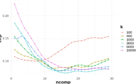
Figure 7 : Classification error of the test set of a KNN-PLSDA, depending on the number of PLS latent variables and the number of neighbours
Figure 7 shows the prediction error of a KNN-PLSDA model as a function of the number of PLS latent variables for a given number of neighbours k ∈ {100,400,1000,3000,5000,10 000}. These results are much better compared to the PLSDA model (see figure 6) with a minimal prediction error divided by 2.5. This confirms the non-linearity within the data.
Number of neighbours Optimal number of LVs Misclassification error (%) 100 7 10 400 13 8 1000 14 8 3000 16 7 5000 14 8 10000 22 8
Table 1 summarises the minimum misclassification errors and the associated latent variables depending on the size of the considered neighbourhood (from figure 7). It illustrates that as the number of neighbours increases, errors decrease but with a growing optimal number of latent variables. Table 1 shows that the minimum prediction error is 7% for an optimal number of neighbours of 3000 and a number of latent variables of 16. It can then be concluded that the KNN-PLSDA method for this study is more efficient than the PLSDA. Furthermore, it is observed that to achieve minimal prediction errors, it is necessary to create KNN-PLS models with a large number of PLS latent variables, which means that genotype discrimination is difficult to achieve.
In this section, two points will be discussed : the neighbourhood of samples and the prediction error of the parSketch-PLSDA method.
Figure 8 : Heatmap of the number of predictable samples found by parSketch, as a function of the 3 parameters v, s, m (number of random vectors, number of segments, minimum % of grids). Figure 8 is divided into 4 graphs, each graph corresponds to a value of parameter m.
For each sample in the test set, parSketch returns a neighbourhood whose size depends on the parameters of the algorithm. An sample in the test set is said to be predictable, if the neighbourhood returned by parSketch contains at least 30 samples.
Figure 8 shows that the number of predictable samples decreases as the value of m increases. The parameter m is used to select the samples most often present in the same cell as the sample to be predicted (see section 2). The parSketch method constructs grids on sketches
that are derived from matrix P random vectors. It is therefore very unlikely to obtain a large number of neighbours if the threshold m is too high (Cf section 2.2).
Figure 8 shows that the number of predictable samples decreases as the values of s (number of segments) and v (number of random vectors) increase. s defines the number of cells in each grid (see section 2). When the number of cells in each grid increases, the cells are smaller and therefore contain fewer samples.
The number of random vectors (v) is used to preserve the Euclidean distances in an approximate way. This parameter is not directly related to the size of the neighbourhood but v is linked to the threshold m and thus will have an indirect impact on the number of predictable samples.
To conclude, s and m have a strong impact on the number of predictable samples while v has a weak (indirect) impact on the number of predictable samples.
Figure 9 : Distribution of the number of neighbours per test sample as a function of the parSketch parameters (v, m, s).
Figure 9 shows that when the value of parameters m and s is too high, the number of returned neighbours is low or even zero. Moreover, a highly stochastic behaviour of the neighbourhood distributions can be observed when the value of the threshold m is high (e.g. m = 90%). In addition, when m has values that are too high, the impacts of other factors are not observable.
It is therefore not possible to make conclusions about the influence of the parSketch parameters when the value of the parameters m and s are too high. For future observations, the distributions of the neighbourhoods obtained with parameters m = 90 or s = 15 are not studied.
In Figure 9, it is possible to observe the impact of the three parSketch parameters on the neighbourhood distributions of the samples to be predicted.
Firstly, when v varies, the median number of neighbours and the interquartile range of neighbourhoods are constant. Indeed, the number of random vectors has no impact on the quantity of returned neighbours (see section 2).
Secondly, as s increases, the median number of neighbours per sample to be predicted decreases. Indeed, s defines the number of cells in each grid, the more s will have a high value the more cells there will be and thus the fewer samples in each cell. When s increases, the interquartile range of neighbourhoods decreases. Indeed, the stronger the segmentation, the less influence there will be on the structure of the position of the samples to be predicted in the database.
Thirdly, when m increases, the median number of neighbours and the interquartile neighbourhood gap per sample decreases. m is a threshold, the higher the value of m the
more similar the samples returned by parSketch will be. Therefore, if the value of m is high, fewer neighbours will be returned by parSketch.
To conclude, with the help of figures 8 and 9 it is possible to eliminate certain combinations of parameters. Indeed, figure 8 makes it easy to select combinations that allow us to predict a certain number of samples. Then, figure 9 allows the selection of combinations of parameters according to the characteristics of the neighbourhoods (e.g. a high number of neighbours and a low variability of the neighbourhoods). Five combinations were chosen to calculate a PLSDA model (see Table 2).
Table 2 : Combinations of the selected parSketch parameters
Combinaison m v s 1 50 10 9 2 50 10 11 3 50 20 11 4 50 20 11 5 50 100 13
These combinations of parameters were chosen because the resulting neighbourhoods were small and all samples were predictable. However, in these combinations, the median
neighbourhood returned by parSketch is much larger (100,000) than the neighbourhood used in the KNN-PLSDA, which was 3,000 neighbours.
Figure 10 : Method classification error : parSketch-PLSDA (all 5 combinations); PLSDA and KNN-PLSDA (3000 neighbours), depending on the number of PLS latent variables
In Figure 10, the error curves of the parSketch-PLSDA are all very close and provide an optimal error of approximately 10%. Figure 10 shows parSketch-PLSDA provides better prediction than PLSDA. The best combination of parameters approaches the best result of the KNN-PLSDA. To conclude, on the example discussed in the article, the neighbourhood returned by parSketch may provide an alternative. ParSketch provides a neighbourhood that allows us to improve the prediction qualities but this neighbourhood can be very large and therefore not all the neighbours returned by pasketch are useful.
This article shows that the combination of a big-data indexing algorithm (parSketch) with PLSDA (parsketch-PLSDA) approaches the best results of KNN-PLSDA on the treated example (wheat leaf genotype discrimination by hyperspectral imaging). The parSketch method is not able to obtain as good classification results as the KNN-PLSDA method, but allows better results than a PLSDA. It can be concluded that parSketch-PLS is very efficient in terms of computation time to select neighborhoods in massive datasets and allows to handle non-linear relations between X and Y. ParSketch is less efficient than the brute-force method to obtain relevant neighbours for PLS model calculation, but allows to realise a fast estimation of the neighbourhood on massive databases. The KNN-PLS and parSketch-PLS methods are used in real time, i.e. for each prediction to be performed a PLS model is calculated on the selected neighborhood and the prediction is directly performed. The prediction of the 400 test samples took several hours with KNN-PLS while the prediction using parSketch-PLS took only a few minutes. This article also shows that it is possible to use parSketch to study the database. Indeed, the parameters s and m (number of segments and minimum % of grids) are dependent on the database structure, for example if the database is very compact, the neighbourhoods returned by parSketch will be very large. In order to confirm the feasibility study a real application will be realised in a second step with the parSketch-PLS method. A major problem with parSketch is that it may return too large neighbourhoods. If the neighbourhoods returned by parSketch are too large, it is possible to fail to handle non-linearity. Indeed, if too many neighbours are returned it is possible that these samples do not all belong to the same linear model. Moreover, the computation time of a PLS model is related to the number of samples. A solution to obtain smaller neighbourhoods and better predictions is to combine parSketch with a method for selecting samples. For example, parSketch could be combined with the brute-force method to reduce the number of distances to be computed for each sample to predict. This means that within a neighbourhood returned by parSketch it would be possible to apply the brute force method. It would therefore be interesting to study parSketch as a filter and then to combine parSketch with another approach of selection or weighting of samples.
6.
Acknowledgements
This work was supported by the French National Research Agency under the Investments for the Future Program, referred as ANR-16-CONV-0004.
The authors want to thank Oleksandra Levchenko for the productive discussions and relevant insights regarding the parSketch approach and its application to various domains, including chemometrics.
7.
References
[1] S. Wold, M. Sjöström, et L. Eriksson, « PLS-regression: a basic tool of
chemometrics », Chemom. Intell. Lab. Syst., vol. 58, no 2, p. 109‑ 130, oct. 2001,
doi: 10.1016/S0169-7439(01)00155-1.
[2] P. Dardenne, G. Sinnaeve, et V. Baeten, « Multivariate Calibration and Chemometrics for near Infrared Spectroscopy: Which Method? », J. Infrared
Spectrosc., vol. 8, no 4, p. 229‑ 237, oct. 2000, doi: 10.1255/jnirs.283.
[3] F. Davrieux et al., « LOCAL Regression Algorithm Improves near Infrared Spectroscopy Predictions When the Target Constituent Evolves in Breeding Populations »:, J. Infrared Spectrosc., janv. 2016, doi: 10.1255/jnirs.1213.
[4] M. Clairotte et al., « National calibration of soil organic carbon concentration using diffuse infrared reflectance spectroscopy », Geoderma, vol. 276, p. 41‑ 52, août 2016, doi: 10.1016/j.geoderma.2016.04.021.
[5] D. Pérez-Marín, A. Garrido-Varo, et J. E. Guerrero, « Non-linear regression methods in NIRS quantitative analysis », Talanta, vol. 72, no 1, p. 28‑ 42, avr.
2007, doi: 10.1016/j.talanta.2006.10.036.
[6] M. Bevilacqua et F. Marini, « Local classification: Locally weighted–partial least squares-discriminant analysis (LW–PLS-DA) », Anal. Chim. Acta, vol. 838, p. 20‑ 30, août 2014, doi: 10.1016/j.aca.2014.05.057.
[7] A. M. C. Davies, H. V. Britcher, J. G. Franklin, S. M. Ring, A. Grant, et W. F. McClure, « The application of fourier-transformed near-infrared spectra to
quantitative analysis by comparison of similarity indices (CARNAC) », Mikrochim.
Acta, vol. 94, no 1‑ 6, p. 61‑ 64, janv. 1988, doi: 10.1007/BF01205839.
[8] K. Hazama et M. Kano, « Covariance-based locally weighted partial least squares for high-performance adaptive modeling », Chemom. Intell. Lab. Syst., vol. 146, p. 55‑ 62, août 2015, doi: 10.1016/j.chemolab.2015.05.007.
[9] B. Igne, J. B. Reeves, G. McCarty, W. D. Hively, E. Lund, et C. R. Hurburgh, « Evaluation of Spectral Pretreatments, Partial Least Squares, Least Squares Support Vector Machines and Locally Weighted Regression for Quantitative Spectroscopic Analysis of Soils », J. Infrared Spectrosc., vol. 18, no 3, p.
167‑ 176, juin 2010, doi: 10.1255/jnirs.883.
[10] Tormod. Naes, Tomas. Isaksson, et Bruce. Kowalski, « Locally weighted regression and scatter correction for near-infrared reflectance data », Anal.
Chem., vol. 62, no 7, p. 664‑ 673, avr. 1990, doi: 10.1021/ac00206a003.
[11] D. Andueza, F. Picard, D. Dozias, et J. Aufrère, « Fecal Near-Infrared
Reflectance Spectroscopy Prediction of the Feed Value of Temperate Forages for Ruminants and Some Parameters of the Chemical Composition of Feces:
Efficiency of Four Calibration Strategies »:, Appl. Spectrosc., juin 2017, doi: 10.1177/0003702817712740.
[12] C. Ariza-Nieto, O. Mayorga, B. Mojica, D. Parra, et G. Afanador-Tellez, « Use of LOCAL algorithm with near infrared spectroscopy in forage resources for grazing systems in Colombia », J. Infrared Spectrosc., vol. 26, no 1, p. 44‑ 52, févr. 2018,
doi: 10.1177/0967033517746900.
[13] P. Berzaghi, J. S. Shenk, et M. O. Westerhaus, « LOCAL Prediction with near Infrared Multi-Product Databases », J. Infrared Spectrosc., vol. 8, no 1, p. 1‑ 9,
janv. 2000, doi: 10.1255/jnirs.258.
[14] I. I. F. E. Barton, J. S. Shenk, M. O. Westerhaus, et D. B. Funk, « The Development of near Infrared Wheat Quality Models by Locally Weighted Regressions »:, J. Infrared Spectrosc., févr. 2017, doi: 10.1255/jnirs.280.
[15] J. A. Fernández Pierna et P. Dardenne, « Soil parameter quantification by NIRS as a Chemometric challenge at ‘Chimiométrie 2006’ », Chemom. Intell. Lab. Syst., vol. 91, no 1, p. 94‑ 98, mars 2008, doi: 10.1016/j.chemolab.2007.06.007.
[16] E. Fernández-Ahumada et al., « Reducing NIR prediction errors with nonlinear methods and large populations of intact compound feedstuffs », Meas. Sci.
Technol., vol. 19, no 8, p. 085601.
[17] E. Fernández-Ahumada, T. Fearn, A. Gómez-Cabrera, J. E. Guerrero-Ginel, D. C. Pérez-Marín, et A. Garrido-Varo, « Evaluation of Local Approaches to Obtain Accurate Near-Infrared (NIR) Equations for Prediction of Ingredient Composition of Compound Feeds », Appl. Spectrosc., vol. 67, no 8, p. 924‑ 929, août 2013, doi:
[18] J. S. Shenk, M. O. Westerhaus, et P. Berzaghi, « Investigation of a LOCAL Calibration Procedure for near Infrared Instruments », J. Infrared Spectrosc., vol. 5, no 4, p. 223‑ 232, oct. 1997, doi: 10.1255/jnirs.115.
[19] G. Sinnaeve, P. Dardenne, et R. Agneessens, « Global or Local? A Choice for NIR Calibrations in Analyses of Forage Quality », J. Infrared Spectrosc., vol. 2, no
3, p. 163‑ 175, juin 1994, doi: 10.1255/jnirs.43.
[20] M. Barker et W. Rayens, « Partial least squares for discrimination », J. Chemom., vol. 17, no 3, p. 166‑ 173, 2003, doi: 10.1002/cem.785.
[21] T. Fearn et A. M. C. Davies, « Locally-Biased Regression », J. Infrared
Spectrosc., vol. 11, no 6, p. 467‑ 478, déc. 2003, doi: 10.1255/jnirs.397.
[22] F. Gogé, R. Joffre, C. Jolivet, I. Ross, et L. Ranjard, « Optimization criteria in sample selection step of local regression for quantitative analysis of large soil NIRS database », Chemom. Intell. Lab. Syst., vol. 110, no 1, p. 168‑ 176, janv.
2012, doi: 10.1016/j.chemolab.2011.11.003.
[23] R. Bayer, « Binary B-trees for Virtual Memory », in Proceedings of the 1971 ACM
SIGFIDET (Now SIGMOD) Workshop on Data Description, Access and Control,
New York, NY, USA, 1971, p. 219–235, doi: 10.1145/1734714.1734731.
[24] J. L. Bentley, « Multidimensional binary search trees used for associative searching », Commun. ACM, vol. 18, no 9, p. 509‑ 517, sept. 1975, doi:
10.1145/361002.361007.
[25] R. A. Finkel et J. L. Bentley, « Quad trees a data structure for retrieval on composite keys », Acta Inform., vol. 4, no 1, p. 1‑ 9, mars 1974, doi:
[26] A. Guttman, « R-trees: A Dynamic Index Structure for Spatial Searching », in
Proceedings of the 1984 ACM SIGMOD International Conference on Management of Data, New York, NY, USA, 1984, p. 47–57, doi: 10.1145/602259.602266.
[27] N. Roussopoulos, S. Kelley, et F. Vincent, « Nearest Neighbor Queries », in
Proceedings of the 1995 ACM SIGMOD International Conference on Management of Data, New York, NY, USA, 1995, p. 71–79, doi: 10.1145/223784.223794.
[28] I. Assent, R. Krieger, F. Afschari, et T. Seidl, « The TS-Tree: Efficient Time Series Search and Retrieval », p. 12.
[29] Y. Cai et R. Ng, « Indexing spatio-temporal trajectories with Chebyshev
polynomials », in Proceedings of the 2004 ACM SIGMOD international conference
on Management of data - SIGMOD ’04, Paris, France, 2004, p. 599, doi:
10.1145/1007568.1007636.
[30] A. Camerra, J. Shieh, T. Palpanas, T. Rakthanmanon, et E. Keogh, « Beyond one billion time series: indexing and mining very large time series collections with iSAX2+ », Knowl. Inf. Syst., vol. 39, no 1, p. 123‑ 151, avr. 2014, doi:
10.1007/s10115-012-0606-6.
[31] A. Camerra, T. Palpanas, J. Shieh, et E. Keogh, « iSAX 2.0: Indexing and Mining One Billion Time Series », in 2010 IEEE International Conference on Data Mining, Sydney, Australia, 2010, p. 58‑ 67, doi: 10.1109/ICDM.2010.124.
[32] C. Faloutsos, M. Ranganathan, et Y. Manolopoulos, « Fast Subsequence Matching in Time-Series Databases », p. 11.
[33] T. Rakthanmanon et al., « Data Mining a Trillion Time Series Subsequences Under Dynamic Time Warping », p. 5.
[34] J. Shieh et E. Keogh, « iSAX: disk-aware mining and indexing of massive time series datasets », Data Min. Knowl. Discov., vol. 19, no 1, p. 24‑ 57, août 2009,
doi: 10.1007/s10618-009-0125-6.
[35] Y. Wang, P. Wang, J. Pei, W. Wang, et S. Huang, « A data-adaptive and dynamic segmentation index for whole matching on time series », Proc. VLDB Endow., vol. 6, no 10, p. 793‑ 804, août 2013, doi: 10.14778/2536206.2536208.
[36] D. E. Yagoubi, R. Akbarinia, F. Masseglia, et T. Palpanas, « DPiSAX: Massively Distributed Partitioned iSAX », in 2017 IEEE International Conference on Data
Mining (ICDM), New Orleans, LA, 2017, p. 1135‑ 1140, doi: 10.1109/ICDM.2017.151.
[37] O. Levchenko, D.-E. Yagoubi, R. Akbarinia, F. Masseglia, B. Kolev, et D. Shasha, « Spark-parSketch: A Massively Distributed Indexing of Time Series Datasets », in
Proceedings of the 27th ACM International Conference on Information and Knowledge Management - CIKM ’18, Torino, Italy, 2018, p. 1951‑ 1954, doi:
10.1145/3269206.3269226.
[38] D. E. Yagoubi, R. Akbarinia, F. Masseglia, et D. Shasha, « RadiusSketch: Massively Distributed Indexing of Time Series », in 2017 IEEE International
Conference on Data Science and Advanced Analytics (DSAA), Tokyo, Japan,
2017, p. 262‑ 271, doi: 10.1109/DSAA.2017.49.
[39] W. B. Johnson, J. Lindenstrauss, et G. Schechtman, « Extensions of lipschitz maps into Banach spaces », Isr. J. Math., vol. 54, no 2, p. 129‑ 138, juin 1986, doi:
10.1007/BF02764938.
[40] C. M. Bishop, Pattern recognition and machine learning. New York: Springer, 2006.
[41] R. W. Kennard et L. A. Stone, « Computer Aided Design of Experiments »,
Technometrics, vol. 11, no 1, p. 137‑ 148, févr. 1969, doi:
10.1080/00401706.1969.10490666.
[42] « R Core Team (2019). R: A language and environment for statistical computing. R Foundation for Statistical Computing, Vienna, Austria. URL https://www.R-project.org/. »
[43] M. Lesnoff, M. Metz, et J.-M. Roger, « Comparison of locally weighted PLS strategies for regression and discrimination on agronomic NIR data », J.
Chemom., vol. n/a, no n/a, p. e3209, doi: 10.1002/cem.3209.
[44] G. Shen et al., « Local partial least squares based on global PLS scores », J.
Chemom., vol. 33, no 5, p. e3117, 2019, doi: 10.1002/cem.3117.
8. Figure Captions
Figure 1 : Sketch creation
Figure 2 : Grid creation
Figure 3 : neighbour search
Figure 4 : spectra plot of the 4 genotypes
Figure 5 : Plot of the first two PCA scores
Figure 6 : Error in classification of the test set according to the number of latent variables PLS
Figure 7 : Classification error of the test set of a KNN-PLSDA, depending on the number of PLS latent variables and the number of neighbours
Figure 8 : heatmap of the number of predictable samples found by parSketch, as a function of the 3 parameters v, s, m (number of random vectors, number of segments, minimum % of grids). Figure 8 is divided into 4 graphs, each graph corresponds to a value of parameter m.
Figure 9 : Distribution of the number of neighbours per test sample as a function of the parSketch parameters (v, m, s).
Figure 10 : Method classification error : parSketch-PLSDA (all 5 combinations); PLSDA and KNN-PLSDA (3000 neighbours), depending on the number of PLS latent variables.