HAL Id: hal-02559874
https://hal.archives-ouvertes.fr/hal-02559874
Submitted on 30 Apr 2020
HAL is a multi-disciplinary open access
archive for the deposit and dissemination of
sci-entific research documents, whether they are
pub-lished or not. The documents may come from
teaching and research institutions in France or
abroad, or from public or private research centers.
L’archive ouverte pluridisciplinaire HAL, est
destinée au dépôt et à la diffusion de documents
scientifiques de niveau recherche, publiés ou non,
émanant des établissements d’enseignement et de
recherche français ou étrangers, des laboratoires
publics ou privés.
Lithology, landscape structure and management practice
changes: Key factors patterning vineyard soil erosion at
metre-scale spatial resolution
Emmanuel Chevigny, Amélie Quiquerez, Christophe Petit, Pierre Curmi
To cite this version:
Emmanuel Chevigny, Amélie Quiquerez, Christophe Petit, Pierre Curmi. Lithology, landscape
struc-ture and management practice changes: Key factors patterning vineyard soil erosion at metre-scale
spatial resolution. CATENA, Elsevier, 2014, 121, pp.354-364. �10.1016/j.catena.2014.05.022�.
�hal-02559874�
Lithology, landscape structure and management practice changes: Key
factors patterning vineyard soil erosion at metre-scale spatial resolution
Emmanuel Chevigny
a,⁎
, Amélie Quiquerez
a, Christophe Petit
b, Pierre Curmi
ca
UMR CNRS 6298 ARTeHIS, University of Burgundy, 6 Bd Gabriel, F-21000 Dijon, France bUMR 7041 ArScAn, University of Paris 1 Panthéon-Sorbonne, 3 rue Michelet, F-75006 Paris, France c
Agrosup, UMR 1347 Agroécologie, BP 86510, F-21000 Dijon, France
a b s t r a c t
a r t i c l e i n f o
Article history: Received 2 July 2013
Received in revised form 15 April 2014 Accepted 20 May 2014
Available online xxxx
Keywords: Erosion pattern 1 m-scale resolution Historical landscape structure Land use changes
Vineyards
Dendrogeomorphology
In vineyards, soil erosion is controlled by complex interactions between geomorphological and anthropogenic factors, leading to intra-plot spatial topsoil heterogeneities that are observed at a 1-m scale. This study explores the relative impacts of slope, lithology, historical landscape structure and present-day management practices on soil erosion on vineyard hillslopes. The selected plot is located in the Monthelie vineyard hillslopes (Côte de Beaune, France), where intensive erosion occurs during high-intensity rainfall events. Soil erosion quantification was performed at a square metre scale using dendrogeomorphology. For the same plot, planted in 1972, an initial erosion map was drawn in 2004, with a second map being produced in 2012. These two maps, combined with lithology and slope data, the evolution of landscape structure and the evolution of management practices allow the driving factors of water erosion to be assessed. From the 2004 erosion map, we observed that the spatial distribution of erosion, for the thirty-year period after planting, was mainly controlled by lithology and historical landscape structure, whatever the slope. By subtracting 2004 data from the 2012 data, and thus evaluating ero-sion over the last decade, we discovered that the eroero-sion rate had increased significantly, that spatial distribution of erosion had changed and is now basically controlled by slope steepness and present-day vineyard manage-ment practices. Erosion patterns for the last decade show that the impact of historical landscape structure is grad-ually declining. This study shows that it is crucial to take into account the pre-plantation history of vineyard plots and management practices to further increase our understanding of the spatial distribution of erosion on vineyard hillslopes.
©
1. Introduction
Cultivated hillslopes undergo substantial soil loss, specifically in vineyards where erosion rates range from 10 to 1000 t ha−1year−1, and where soil thickness decreases considerably (Cerdan et al., 2010; Kosmas et al., 1997; Martínez-Casasnovas et al., 2002; Novara et al., 2011). In this context, soil loss has a major economic impact for wine-growers, since gullies must befilled, uprooted vine stocks must be replanted, and soil deposited at the bottom of the plot must be moved back up to the top (Brenot, 2007; Martínez-Casasnovas and Ramos, 2006; Martínez-Casasnovas et al., 2005).
On sloping surfaces, soil loss is associated to a net redistribution of soil within the plot, controlled by the interaction of factors such as to-pography, climate, land use and soil management practices (Chartin et al., 2011; Fox and Bryan, 2000; García-Ruiz, 2010; Lagacherie et al., 2006). Erosion preferentially affects thefine soil fraction, leaving behind
rock fragments and thus proportionately increasing topsoil stoniness (Poesen et al., 1994). Climate and relief (lithology, slope length and slope steepness) are the main factors involved in soil erosion, which plays an important role in topsoil redistribution down the hillslope (Fox and Bryan, 2000). These factors influence both soil volume and the morphology of water-erosive structures, such as linear rill and gully networks (Quiquerez et al., 2008). As a result, the formation of rill systems through which sediment is exported plays a decisive role in conditioning sediment availability and the spatial distribution of eroded soil at the slope scale.
Past and present-day anthropogenic factors (landscape structure and management practices) may also affect topsoil variability and erosion rates (Blavet et al., 2009; García-Ruiz, 2010). In the vineyard context, the influence of present-day weed management practices on topsoil erosion is recognized. Among them, the effects of the most usual practices i.e. no-tillage with chemical weeding (NT) and surface tillage (ST) are still debated. These contradictory results may be ex-plained by the differences existing between the erosion measurement techniques, soil surface condition, climate or topography. Some studies suggests that NT accelerates erosion rate (Raclot et al., 2009) while,
⁎ Corresponding author. Tel.: +33 3 80395791; fax: +33 3 80395787. E-mail address:[email protected](E. Chevigny).
others studies propose that ST management increases erosion rate (Gómez et al., 2008; Le Bissonnais and Andrieux, 2006). The use of mechanisation may locally influence the soil compaction, by decreasing infiltrability which may lead to the formation of rills (Lagacherie et al., 2006). Tillage erosion contributes to net topsoil redistribution across the landscape, by eroding the upper slope and causing soil accumulation downslope (Van Oost et al., 2000). Historical landscape structure may also affect the spatial distribution and erosion rate (Chartin et al., 2011). Soil redistribution is greatly affected by the presence of existing but also historical landscape structure, where hotspot areas of erosion (on undulations) and deposition (on lynchets) have been identified.
Therefore, it is important not only to estimate sediment budgets, but also to perform detailed analyses of erosion patterns at a high spatial resolution of a few metres to better constrain the factors controlling soil degradation. In the short term, these factors modify soil characteris-tics (stoniness and available water) which could influence vine vegeta-tive growth, while in the long term, they may affect soil sustainability.
Intra-plot soil erosion at a high spatial resolution can be derived from “surface elevation change-based” methods, but only for very specific tem-poral scales, e.g. for a single rainstorm event within experimental plots (Martínez-Casasnovas et al., 2005), or for an annual time scale over hillslopes (Sirvent et al., 1997). Spatially distributed soil erosion can also be estimated using geochemical methods, such as radio-nuclide measure-ments 137Cs which are used to trace sediment movement along cross-sections at a decennial time scale (Krause et al., 2003; Walling and Quine, 1991). Temporally and spatially distributed data can be inferred from the identification of bio-markers, using dendrogeomorphology methods, which have proven very useful to estimate erosion rates (Bodoque et al., 2005; Carrara and Carroll, 1979; Casalí et al., 2009; Vanwalleghem et al., 2010). Aggradation or degradation processes are di-rectly inferred from the position of the root collar, considered as afixed spatial reference, relatively to the current ground surface. These methods were adapted byBrenot et al. (2008)for vineyard contexts, and have since been used to quantify erosion in a Spanish vineyard (Casalí et al.,
2009), in a southern French vineyard (Paroissien et al., 2010) and in a Burgundian vineyard (Quiquerez et al., 2014).
Our work investigates the impact of geomorphological (lithology and slope) and anthropogenic (historical landscape structure and man-agement practices) factors controlling topsoil erosion at metre-scale in a vineyard plot. For this purpose, we studied a one-hectare hillslope vineyard plot planted in 1972, and still cultivated by the same wine-grower, for which historical land use data were available for the last two centuries. Lithology, slope, and erosion were mapped at a metre-scale to assess the influence of geomorphological factors on erosion. Two erosion maps were measured in 2004 and in 2012, allowing spatial quantification of erosion over two periods, i.e. respectively period. The 1972–2004 and 2004–2012 periods differ by their weed control man-agement practices. These maps were compared to historical landscape structure to analyse erosion patterns and rates over time. This study re-veals the complex and changing interactions between geology, slope, present-day vineyard management practices and the remaining effects of historical landscape structure.
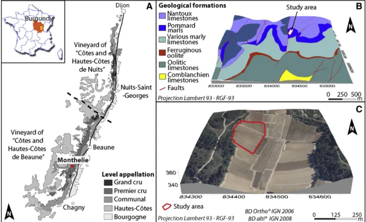
2. Material and methods 2.1. Study area
The study area is located on the hillslopes of Monthelie (Fig. 1A), in the Côte de Beaune area (Burgundy, France). This 1.1 ha vineyard plot lies on the western side of a north-oriented valley, cross-cutting the Jurassic formations of the Burgundian plateau (Rémond, 1985) (Fig. 1B and C). According to the WRB classification (IUSS Working Group WRB, 2006), the soil is a stony silty clay Calcaric Cambisol which developed on Jurassic marls. Topsoil contents 35% calcareous gravel and stones, 7.1% mean organic matter, 48% calcium carbonate content, and pH is 8.1. Topsoil bulk density ranges from 1.25 to 1.5 g cm−3depending on row or inter-row position (Brenot et al., 2008). Since the last plantation in 1972, the plot has always been cultivated by the same wine-grower.
Before plantation, the plot was ploughed to a depth of 40 cm. Soil man-agement practices vary from no-tillage and chemical weeding (NT) till the nineties and surface tillage (ST), without grass cover throughout the year.
2.1.1. Mapping lithology and estimating topsoil stoniness
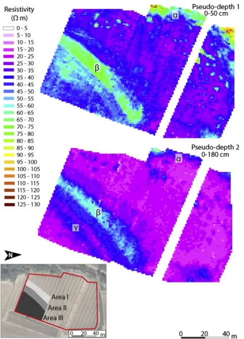
Lithology was mapped by processing the geophysical data acquired on 29th March 2012 using the Automatic Resistivity Profiling method (ARP©,Dabas, 2008). To measure apparent electrical resistivity, the acquisition device was installed on a straddle tractor coupled with a dGPS providing spatial position data (Panissod et al., 1998). All rows were prospected to produce very high spatial resolution maps (37 points/m2). Raw data werefiltered and then interpolated (2D bicubic spline interpolation) to map of soil apparent resistivity at a resolution of 1 m2. Apparent resistivity was measured for two investigation depths, i.e. 0–50 cm (pseudo-depth 1) and 0–180 cm (pseudo-depth 2), to assess changes in soil or lithology (Fig. 2).
Topsoil stoniness was estimated by dry sieving on undispersed ma-terial. Samples were collected in the 0–5 cm soil layer in the inter-row, over a 0.25 m2surface, corresponding to a volume of 10 l. Ten samples were collected from all over the plot:five in low erosion areas and five in high erosion areas.
2.1.2. Slope and waterflow directions
A digital elevation model (DEM) was constructed using dGPS with decimetric altitudinal precision at a 10 m spatial resolution. This DEM was used to map the slope and the direction of waterflow (Fig. 3). Elevation decreases from 369 m at the edge of the plateau, to 340 m downslope. From the plateau border at the north-western part of the plot slopes range from 2° to 15°, while steep slopes occupy the south-eastern part of the plot and may reach up to 21° (Fig. 3A). Waterflow directions, determined from the DEM, are oriented respectively towards the SE in the northern part of the plot and towards ESE in the southern part of the plot (Fig. 3B). Everywhere in the plot, the directions of water flow differ from those of the vine rows (e.g. WE direction). Since the
last plantation in 1972, the plot has been cultivated by the same wine-grower since this date (Fig. 3B). Before the plantation, the wine-grower has performed a deep ploughing (40 cm deep) all over the plot. 2.2. Mapping erosion
The principle of soil loss measurement is similar to that used in dendrogeomorphology methods, and is based on the unearthing of the stock located on the vine plants (Stock Unearthing Measurement, or SUM), considered as a passive marker of soil surface vertical displace-ment since the year of plantation (Brenot et al., 2008). Grafting vines has been compulsory since the Phylloxera crisis at the end of the 19th century. Vine anatomy divided in two components: the“American” rootstock and the aerial scion. Removing the germination from the root-stocks prevents any vertical stock growth, while the scion will grow in all directions (Brenot et al., 2008). At plantation, the graft-union is planted at 1 cm above the soil level, in order to prevent contact between the scion and the soil.Brenot et al. (2008)verified that the vertical growth of the graft after plantation is minimal and therefore that the distance between the soil and the graft-union is representative of soil loss. The plantation legislation in Burgundian vineyards imposes a den-sity of 10,000 vine stocks per hectare which allows the quantification of erosion at a 1-m scale over pluri-decennial periods with an error margin of 1 cm related to the plantation method (Brenot et al., 2008). Erosion
rate can be calculated at a 1-m scale by dividing the SUM by the age of the vines.
Two SUM campaigns were conducted in winter 2004 and in spring 2012. Each vine stock was measured twice, allowing erosion rate and spatial distribution variation to be detected. Only the SUMs of vine stocks initially planted in 1972 were taken into account to ensure data reliability; stocks absent or replaced after 1972 were simply located on the plot (Fig. 4). In winter 2004, 9384 SUMs were performed by
Brenot (2007)and 1925 vine stocks were absent or too young to be measured (Table 1). In spring 2012, only 7336 vine SUMs were per-formed, since 421 vine stocks onfive rows were uprooted in 2006 and the others were young or absent; as soil infilling was performed on 135 vine stocks in the eastern part of the plot in 2008, these vine stocks were also excluded. Most of the vine stocks with SUMs higher than 15 cm in 2004 were either absent or replaced by young vines in 2012, corresponding to the loss of 1324 vine stocks in 8 years, caused by erosion or disease. The loss of vine stocks with high SUMs leads to an underestimation of erosion.
2.3. Historical land use datasets
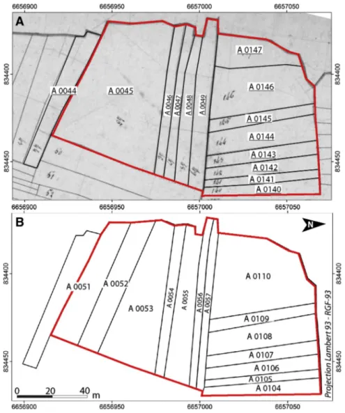
The landscape structure is characterised by a vine monoculture where plot limits, i.e. walls and paths, have formed the discontinuities along the hillslopes for the last two centuries. These plot limits have been partly deleted with the advent of mechanisation in the 20th centu-ry. Therefore, we used two cadastral maps to characterise landscape structure evolution over the last two centuries (Fig. 5): the 1825 “Napo-leonic cadastre”, “Section A1 1st sheet” (AD21, 2006) (Fig. 5A) and the 1932“BD Parcellaire”, “Sheet 000 A1” (IGN, 2008a) (Fig. 5B), both drawn at a 1/2500 scale. Cadastral matrices were consulted to the Monthelie town hall archives. The archive documents contain all the information relative to the owners, the type of land use and the
Fig. 3. Slope map (A) and waterflow direction (B) maps. The length of black arrows indicates slope steepness. Green bands observed on the ortho-photograph indicate grass cover in 2006 on treatment rows. Seven brown points located in the northern part of the plot correspond to piles of vine stocks coming from 5 uprooted rows. (For interpretation of the references to colour in thisfigure legend, the reader is referred to the web version of this article.)
Fig. 4. Map locating data not available for SUM quantification: absent or young vine stocks, uprooted area and anthropogenic soil infilling area.
Table 1
Number of stock unearthing measurements (SUMs) collected during the 2004 and 2012 campaigns.
Date Number of vine stocks Measured Not measured
Young or absent Uprooted Anthropogenic soil infilling 2004 9384 1925
2006 421
2008 135
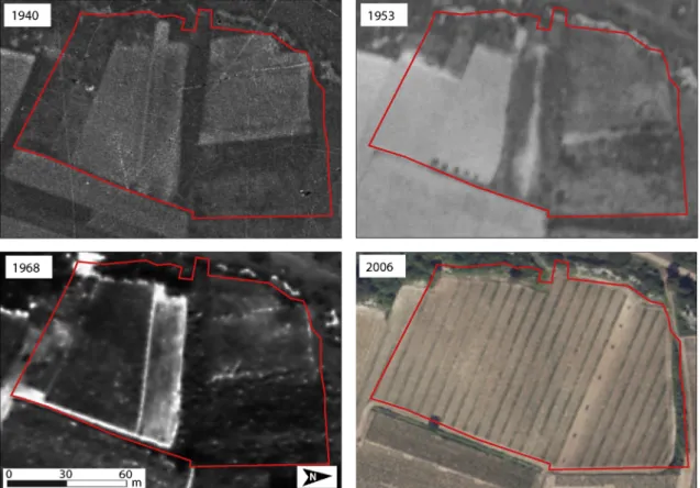
evolution of plot areas. In addition, we used historical and recent aerial photographs, to define the types of plot limits and their spatio-temporal evolution (Fig. 6). We used historical aerial photographs for 1940, 1953 and 1968 (IGN, 2006); and the 2006 ortho-photograph (IGN, 2008b).
The “BD Parcellaire” was georeferenced by the IGN, and the “Napoleonic cadastre” was georeferenced according to common limits with the“BD Parcellaire” map. Historical photographs were georeferenced using anchor points recognisable in the 2006 ortho-photograph (IGN, 2008b).
3. Results 3.1. Lithology
On the apparent resistivity map of pseudo-depth 1, two areasα and β were characterised by high values (Fig. 2). Areaα, extending over the north-western edge of the plot, presented the highest apparent resistiv-ity values, 125Ω m for pseudo-depth 1 and 92 Ω m for pseudo-depth 2. Areaβ, a band 9 m wide, located in the south-eastern part of the plot, was characterised by a linear pattern of high apparent resistivity values, from 70Ω m for pseudo-depth 1 to 55 Ω m for pseudo-depth 2. In pseudo-depth 1, scattered points of high apparent resistivity indicate the presence of dense gravel and stone cover on the topsoil. In
pseudo-depth 2, another linear patternγ was observed, which presented higher apparent resistivity values (mean of 35Ω m) than the surround-ing area. Auger holes in these areas highlighted a change in lithology: a marly-limestone band was present at 20/30 cm depth, while outside these areas the plot was characterised by lower values, most of them ranging from 28 to 42Ω m, which were interpreted as a marly formation. 3.2. Historical evolution of landscape structure
The cadastral maps show the spatial evolution of plot limits (Fig. 5). On the 1825“Napoleonic cadastre”, the study area was divided into fourteen plots (Fig. 5A). The 1825 limits were underlined, to differenti-ate them from those of 1932. The southern part was composed of six plots, with an east-west orientation, referenced A 0044 to A 0049. The northern part included eight plots with a north–south orientation, ref-erenced A 0140 to A 0147. On the 1932“BD Parcellaire”, the study area was also composed of fourteen plots, which differed from those of 1825 (Fig. 5B). Most limits have not changed during this period in the northern part of the study area, even though some changes can be observed in the southern part. Plot division was generally due to an inheritance concerning several heirs (e.g. plots A 0045 and A 0049). The merging of several plots occurred when neighbouring plots were acquired by the same owner (e.g. plots A 0051 and A 0055).
Fig. 5. Cadastral maps of study area, dating from 1825 (A) (Napoleonic cadastre, AD21) and 1932 (B) (BD Parcellaire, IGN). Red line represents present-day cadastral limits. According to cadastral matrix, plot A 0045 was divided into three plots in 1834 and 1863; the southern plot was merged with plot A 0044 to form plot A 0051 in 1932. Plots A 0047 and A 0048 were merged to form plot A 0055 in 1932. In 1869, plot A 0049 was divided into two plots: A 0056 and A 0057. In the northern part, plots A 0146 and A 0147 were merged to form plot A 110. (For interpretation of the references to colour in thisfigure legend, the reader is referred to the web version of this article.)
Historical photographs reveal the use of several types of plot limits over time (Fig. 6). Interpretations of aerial photographs were confirmed by the testimony of the wine-grower. The limit between plots A 0053 and A 0054 matched an agricultural path from 2 to 3 m wide (Fig. 6, 1968). In plot A 0110, the plot limit appears in the form of an alignment of dry stones on the east, west and north boundaries of the plot (Fig. 6, 1968). These alignments, called“murgers” in Burgundy, were dry-stone walls built as the wine-growers removed stones from the plot. The up-slope part of plots A 0051 and A 0052 were not cultivated from 1940 to 1953. The limit between uncultivated and cultivated land is marked by an embankment of 1 m high, which interrupted the slope (Fig. 6, 1953). Before replanting in 1972, this break-in-slope wasfilled in, with soil brought from further down the slope. The north-eastern plot limits, which cannot be observed on aerial photographs, were formed by small furrows dug out by wine-growers when they pickaxed their vines, before mechanisation in the middle of the 20th century. To keep the maximum amount of soil in their plots, they pulled soil in their plot direction, thus creating small depressions between two plots. Others limits were just administrative limits; they indicated a change of ownership or a change in land use.
3.3. Erosion quantification
For the period from 1972 to 2004, the mean SUM was 3.5 cm ± 1 cm (Table 2). The mean erosion rate at the plot scale was estimated to be 1.1 ± 0.3 mm year−1. For the 2004–2012 period, obtained by subtracting the 2004 SUM to the 2012 SUM, the mean SUM was 2.3 ± 1 cm and the erosion rate was estimated to be 2.8 ± 1.3 mm year−1. Our measurements showed that erosion increased significantly for the 2004–2012 period compared the 1972–2004 period (Mann-Whitney U-test, p-valueb0.0001). Erosion rates calculated for the two periods are consistent with estimations in similar vineyard contexts (Casalí et al., 2009; Cerdan et al., 2010; Paroissien et al., 2010).
The datasets for 2004 and 2012 showed that SUM values varied from 0 cm to 26 cm (Fig. 7). For the 2004 data, 33% of SUM values showed no erosion. The SUM distribution was centred on the SUM value of 5 cm. For the 2012 data, only 14% of SUMs showed no erosion and the SUM distribution showed greater dispersion. The evolution of SUM distribu-tions between these two dates shows: (i) an increase of erosion in areas without erosion in 2004 and (ii) a greater number of high erosion values.
Fig. 8shows the two erosion maps 2004 and 2012. Both maps dis-play similar erosion patterns. They differ essentially in erosion intensity. For both maps, it is possible to identify three areas by their erosion patterns (A, B and C). We shall therefore only discuss the results for the 2004 erosion maps.
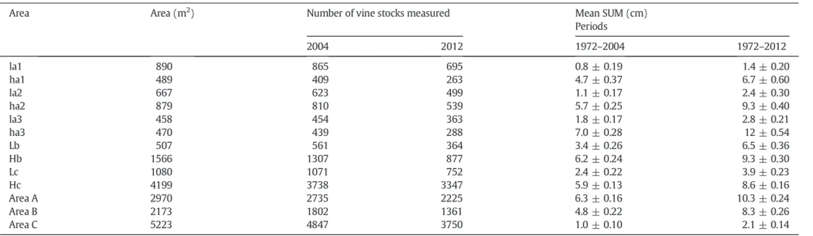
Area A, located in the southern part of the plot, is characterised by low erosion values downslope and by high erosion values upslope. The limits between low and high erosion values were well defined and were oriented along a SSW-NNE and a WNW-ESE directions (reported as limits a1 and a2 inFig. 8C). Upslope from limits a1 and a2, the mean SUMs were respectively 4.7 and 5.7 cm ± 1 cm (see
Fig. 6. Aerial photographs of the study area, from 1940, 1953, 1968 and 2006. On the older photographs, the red line represents present-day cadastral limits. On the western border, the cadastral limits are different from the vineyard plot planted in 1972. (For interpretation of the references to colour in thisfigure legend, the reader is referred to the web version of this article.)
Table 2
Mean SUM and erosion rates calculated for the two periods studied.
Periods Mean SUM Erosion rate
cm mm year−1
1972–2004 3.5 ± 0.08 1.1 ± 0.03 2004–2012 2.3 ± 0.06 2.8 ± 0.08 SUM and erosion values are given with their confidence interval.
areas ha1 and ha2 inFig. 8C). Downslope from the limits, the mean SUMs were respectively 0.8 and 1.1 ± 1 cm (see areas la1 and la2 in
Fig. 8C;Table 3). A third limit, less well defined, with a NW-SE orienta-tion, separated two areas of low/high erosion (limit a3 inFig. 8C). Mean SUM was 1.8 cm ± 1 cm south of the limit (area la3 inFig. 8C) and 7.0 cm ± 1 cm north of the limit (area ha3 inFig. 8C;Table 3).
Area B, in the central part of the plot, displayed linear patterns of erosion with a WE orientation (areas lb and hb inFig. 8C). By“linear pat-terns”, we mean an alignment of high or low SUM data on the erosion map. Alternating low and high SUM values generated linear patterns observed from south to north. Low value patterns were narrower than high value patterns. From the north-eastern part, the SUM increased downslope and reached 24 cm ± 1 cm. In this area, it was possible to identity the spatial continuity of the pronounced SSW-NNE limit ob-served in Area A (limit a2 inFig. 8C). Mean SUM was 3.4 ± 1 cm for low erosion values (areas lb inFig. 8C) and 6.2 ± 1 cm for high erosion values (areas hb inFig. 8C;Table 3).
Area C, situated in the northern part of the plot, was defined by the alternation of low and high erosion values, which formed linear pat-terns with NNW-SSE orientation (areas lc and hc inFig. 8C). Mean SUM was 2.4 cm ± 1 cm for low erosion values (areas lc inFig. 8C) and 5.9 cm ± 1 cm for high erosion values (areas hc inFig. 8C;Table 3).
None of the linear erosion patterns observed in these three areas corresponded to waterflow directions determined from the DEM (Fig. 3B).
4. Discussion
4.1. Lithology and erosion patterns
The comparison of apparent resistivity maps (Fig. 2) and erosion maps (Fig. 8) highlighted the impact of lithology on erosion. The change in soil apparent resistivity from 30 to 70Ω m (Area β in pseudo-depth 2,
Fig. 2B) showed a change in lithology that matched a limestone bed in the Oxfordian marl formation (Fig. 1B). This limestone bed was also cor-related to a change from high to low erosion values, with a SW-NE ori-ented limit on the erosion map, observed in Area A (limit a2 inFig. 8C). In the limestone bed area (area II inFig. 2,Table 3), the mean SUM for 2004 was 4.8 cm ± 1 cm and the topsoil stoniness was 62%. Upslope from the limestone bed area (area I inFig. 2,Table 3), mean SUM for 2004 was 6.3 cm ± 1 cm, and topsoil stoniness was lower (30%). Down-slope from the limestone bed (area III inFig. 2,Table 4), the mean SUM for 2004 was only 1.0 cm ± 1 cm and topsoil stoniness was equal to 42%. Since slope angle values remained more or less constant throughout Area A (from 15° to 20°;Fig. 3A), we suggest that changes in erosion intensity are mainly controlled by changes in lithology. High topsoil stoniness above the limestone bed may locally increase water in filtra-tion, leading to a lower runoff volume, and therefore reducing topsoil erodability (Martínez-Zavala and Jordán, 2008; Poesen et al., 1994; Quiquerez et al., 2014).
Fig. 7. Histograms of SUMs for the 2004 and 2012 datasets. SUM distribution has evolved over the last decade.
Fig. 8. Erosion maps with the 2004 (A) and 2012 (B) datasets interpolated from measured vine stocks. Hatched areas on the 2012 map representsfive rows uprooted in 2006 and a 2008 soil anthropogenic infilling area. Delimitation of erosion patterns observed on both ero-sion maps (C); the delimitation of areas la3 and ha3 matches the 349 to 354 m contour lines.
4.2. Historical landscape structure and linear erosion patterns
The plot limits identified on cadastral plans were overlain on the 2004 erosion map to evaluate their impact on erosion patterns.Fig. 9
shows that most of the cadastral limits were correlated to linear pat-terns of low or high erosion values.
Low erosion patterns were characterised by 1 to 3 m wide bands. For example, the limit between Area A and Area B inFig. 9matched both the administrative limit between A 0045 and A 0046 in the“Napoleonic ca-dastre” (Fig. 5A), the limit between A 0053 and A 0054 in the 1932 map (Fig. 5B), and an agricultural path in 1968 (Fig. 6). The limit between A 0048 and A 0056 (Fig. 9) was superimposed on a linear band of low ero-sion and a natural ditch which acted as a gully in 1953 (Fig. 6). On the north-western part of the study area, a low erosion linear pattern (white line inFig. 9) was correlated to the presence of a“murger” (dry-stone wall) identified on the 1968 aerial photograph (Fig. 6). On plots A 0051 and A 0052, SUM evolved sharply from 4.7 to 0.8 cm ± 1 cm on the 2004 map (Limit a1 inFig. 8C and red line in Fig. 9,
Table 3). This limit between the two areas coincided with the position of a break-in-slope observed in the 1953 aerial photograph (Fig. 6).
Some alternations between bands of low and high erosion can also be observed. On the north-eastern part of Area C,Fig. 9shows a WNW cyclic erosion pattern (plots A 104 to A 108). The transition from one plot to another matched a change from high to low SUM values. We sug-gest that this pattern could be explained by the presence of historical shallow furrows (about 10 cm in depth). The furrows, located at the plot limits, concentrate water from upslope. Erosion is thus highest at the furrow position. Water collected by furrows does notflow in plots surrounding the furrow, so those plots present low erosion values. Although furrows were blurred by deep ploughing before plantation in 1972, erosion is controlled by these historical anthropogenic struc-tures. Historical land-use patterns seem to be important in soil erosion and degradation processes and for landscape development (Szilassi et al., 2006).
Linear bands of high erosion, a few metres wide, are also observed in
Fig. 9. For example, plots A 0056 and A 0109 displayed the highest
Table 3
Mean SUM calculated from the 2004 and 2012 datasets for each erosion pattern.
Area Area (m2) Number of vine stocks measured Mean SUM (cm) Periods 2004 2012 1972–2004 1972–2012 la1 890 865 695 0.8 ± 0.19 1.4 ± 0.20 ha1 489 409 263 4.7 ± 0.37 6.7 ± 0.60 la2 667 623 499 1.1 ± 0.17 2.4 ± 0.30 ha2 879 810 539 5.7 ± 0.25 9.3 ± 0.40 la3 458 454 363 1.8 ± 0.17 2.8 ± 0.21 ha3 470 439 288 7.0 ± 0.28 12 ± 0.54 Lb 507 561 364 3.4 ± 0.26 6.5 ± 0.36 Hb 1566 1307 877 6.2 ± 0.24 9.3 ± 0.30 Lc 1080 1071 752 2.4 ± 0.22 3.9 ± 0.23 Hc 4199 3738 3347 5.9 ± 0.13 8.6 ± 0.16 Area A 2970 2735 2225 6.3 ± 0.16 10.3 ± 0.24 Area B 2173 1802 1361 4.8 ± 0.22 8.3 ± 0.26 Area C 5223 4847 3750 1.0 ± 0.10 2.1 ± 0.14
SUM values are given with their confidence interval.
For area denomination,“l” represents low erosion and “h” represents high erosion. Areas with high and low SUM are significantly different (Mann–Whitney test, p-value b0.05).
Table 4
Mean SUM and erosion rates calculated for each historical plot from the 2004 and 2012 datasets.
Plot reference Area (m2
) Number of vine stocks measured
Mean SUM Erosion rate
Period 1 Period 2 Relative increase from periods 1 to 2
cm (mm year−1) % 2004 2012 2004 2012 72/04 04/12 A 0051 520 490 404 0.8 ± 0.26 1.4 ± 0.33 0.2 ± 0.08 0.7 ± 0.37 250 A 0052 950 814 679 1.5 ± 0.23 3.0 ± 0.37 0.5 ± 0.07 1.8 ± 0.32 260 A 0053 1970 1637 1304 3.2 ± 0.20 7.0 ± 0.32 1.0 ± 0.06 4.8 ± 0.25 380 A 0054 500 392 349 4.8 ± 0.36 9.3 ± 0.47 1.5 ± 0.11 5.6 ± 0.39 273 A 0047 490 351 311 2.8 ± 0.35 6.7 ± 0.35 0.9 ± 0.11 4.9 ± 0.48 444 A 0048 610 461 327 4.0 ± 0.36 7.7 ± 0.45 1.3 ± 0.11 4.3 ± 0.41 231 A 0056 470 305 185 7.6 ± 0.67 10.1 ± 0.75 2.4 ± 0.21 5.5 ± 0.57 129 A 0057 470 376 221 3.2 ± 0.52 5.4 ± 0.67 1.0 ± 0.16 2.5 ± 0.72 150 A 0104 450 214 167 2.0 ± 0.45 1.6 ± 0.41 0.6 ± 0.14 −0.5 ± 0.36 −183 A 0105 330 226 152 4.4 ± 0.52 5.2 ± 0.57 1.4 ± 0.16 1.0 ± 0.54 −29 A 0106 480 426 329 3.4 ± 0.39 4.5 ± 0.46 1.1 ± 0.12 1.4 ± 0.32 27 A 0107 520 405 291 4.0 ± 0.47 5.1 ± 0.52 1.2 ± 0.15 1.4 ± 0.36 17 A 0108 860 770 599 4.5 ± 0.33 6.3 ± 0.37 1.4 ± 0.10 2.1 ± 0.25 50 A 0109 410 370 283 6.5 ± 0.40 8.4 ± 0.49 2.0 ± 0.12 2.4 ± 0.36 20 A 0146 1460 1440 1138 4.1 ± 0.18 6.1 ± 0.25 1.3 ± 0.05 2.4 ± 0.19 85 A 0147 720 707 597 1.7 ± 0.24 3.9 ± 0.32 0.5 ± 0.07 2.7 ± 0.26 440 Area 1 3790 3347 2816 3.6 ± 0.13 6.5 ± 0.22 1.1 ± 0.04 3.7 ± 0.13 236 Area 2 2880 2712 1882 6.1 ± 0.18 8.0 ± 0.22 1.9 ± 0.06 4.2 ± 0.06 121 Area 3 3660 3325 2638 4.2 ± 0.12 5.4 ± 0.15 1.3 ± 0.04 1.5 ± 0.07 15 Sum and erosion values are given with their confidence interval.
erosion values of the study area, with a mean SUM for 2012 greater than 8.4 cm ± 1 cm (Table 4). These two plots overlaid two gullies observed on the 1953 aerial photograph (Fig. 6). Once formed, gullies can contin-ue to generate sediment long after the triggering causes have ceased (Valentin et al., 2005). They are interpreted as preferential paths for runoff and erosion.
The confrontation of historical data and erosion maps shows the resilience of historical landscape structure in the erosion patterns identified. Historical landscape structure still influences the distribution and intensity of erosion, although deep ploughing was performed throughout the area before plantation. Soil redistribution is greatly af-fected by the presence of present-day and also historical landscape structure (Chartin et al., 2011). Among the factors controlling erosion patterns and intensity of erosion, we show that: (i) rock fragments contained in topsoil play a crucial role (Quiquerez et al., 2014), the low erosion observed where historical“murgers” and historical paths were situated can be explained by topsoil stoniness which increased water infiltrability, and reduced splash effect (Martinez-Zavala et al.,
2010; Poesen et al., 1994); and (ii) preferential paths of erosion in flu-ence the distribution and intensity of erosion, historical paths are still active even today, highlighting the resilience of erosion over time. In the studied plot, this work shows that erosion depends not only on slope values but also on historical landscape structures and lithology.
4.3. Evolution of erosion patterns and intensity over the last decade In the Monthelie vineyard, historical landscape structure more than two centuries old influences the spatial distribution and intensity of erosion. In this anthropogenic context, where soils are continually perturbed by vineyard management practices, we evaluate the evolution of erosion patterns and intensity over the last decade (2004 to 2012).
The map of differential SUM, presented inFig. 10, was calculated by subtracting for each vine stocks the 2004 SUM to the 2012 SUM. Differ-ential SUM ranges from 0 to 10 cm and the map highlights three areas with specific patterns of erosion, Areas 1, 2 and 3.
Fig. 9. Cadastral limits overlain on the 2004 erosion map. (For interpretation of the references to color in thisfigure legend, the reader is referred to the web version of this article.)
In Area 1, a relative increase in erosion rate of 236% can be observed (Table 4). The limits controlled by geology and topsoil stoniness (hatched area inFig. 9) or by the historical embankment (red line in
Fig. 9) are preserved. Conversely, linear patterns of low erosion values have been deleted. This area has the steepest slopes in the study area, ranging from 15 to 21° (Fig. 3A). Erosion patterns that were controlled by historical anthropogenic factors are declining, as the impact of topog-raphy and lithology increases.
In Area 2, a relative increase in erosion rate of 121% can be observed. An alternation of linear erosion patterns parallel to rows appears (see black arrows inFig. 10; and ellipses inFig. 11). These linear erosion patterns are present every 6 rows (rows 49, 55, 61, 67, 73 and 79) and were grassed in 2006 (Fig. 6). These treatment rows undergo 5 to 10 ad-ditional passages per year, leading to an increase in topsoil compaction and an increase in rill erosion processes (Ferrero et al., 2005; Lagacherie et al., 2006). In this area, linear erosion patterns correlated to historical landscape structure have completely disappeared. As in Area 1, erosion is no longer controlled by historical landscape structure and now seems to be governed by present-day vineyard management practices.
In Area 3, the increase in erosion rate was + 0.2 mm year−1 (Table 4) and the relative increase in erosion rate is slight (only 15%) highlighting erosional stability. In this area, two patterns can be observed: linear patterns parallel to rows every six rows (rows 109, 115 and 121 inFig. 10; and ellipses inFig. 11) and linear patterns with a NS orientation (Figs. 8 and 9). These patterns highlight a combination of two factors of erosion control, i.e. historical landscape structure (NS orientation) and present-day vineyard management practices (WNW orientation). In this area, characterised by gentle slopes, the impact of historical anthropogenic factors has not completely disappeared.
The comparison between the 2004 and 2012 erosion maps shows that the impacts of historical landscape structure on present-day ero-sion patterns are not erased at the same rate all over the study area. It seems that the lessening impact of historical structures is controlled by slope intensity. For gentle slopes, erosion patterns controlled by his-torical landscape structure are partially preserved. For moderate to steep slopes, erosion is controlled by present-day vineyard manage-ment practices, and historical structures have disappeared. For the steepest slopes, present-day and historical anthropogenic factors have no impact; erosion seems to be controlled only by topography and lithology.
We propose that the increase of erosion rate between the two pe-riods could be related to the change in weed management practices from chemical weeding and no tillage (NT) to surface tillage (ST) in 1992. This hypothesis is consistent with the study performed byLe Bissonnais and Andrieux (2006)who demonstrated that erosion rate increased with the change from NT to ST. We assume that erosion increase can be explained by a change of the wheel compaction occur-ring on inter-rows in vineyard context (Curmi et al., 2006). In NT plots the superficial layer remains compact, which reduces the soil particle detachability and limits erosion. Conversely, in ST plots, the soil tillage modifies the superficial soil structure, composed of a loosened soil
surface overlying a low permeability compact layer, which favours soil erosion during intense rainfall events (Curmi et al., 2010).
5. Conclusion
This study shows that erosion in a vineyard context is controlled by complex interactions between geomorphological processes and histori-cal and present-day anthropogenic factors. More specifically, this work highlights the role of historical anthropogenic structures, such as land-scape structure, with regard to erosion in a vineyard context. Historical landscape structure has an impact on erosion intensity and spatial distribution. Some historical structures, such as dry-stone walls, de-crease erosion, whereas historical gullies inde-crease erosion. Our study also shows that the impact of historical landscape structure generally declines over time. However, in a steep slope context, erosion deletes the effects of both historical and present-day anthropogenic factors. Conversely, the effects of historical landscape structure are partially pre-served when the slope is moderate.
This study demonstrates that it is crucial to take into account the pre-plantation history of plots in order to assess the spatial distribution of erosion, especially on vineyard hillslopes where soil losses have major economic and environmental consequences. The SUM appears to be a useful method to quantify the effects of management practice changes on soil erosion on the long term.
Acknowledgements
This work was made possible by thefinancial support of Burgundy Regional Council (CRB) and the Inter-Professional Bureau of Burgundy Wines (BIVB). We offer special thanks to Michel and Sébastien Deschamps, the wine-growers, for their material assistance and for all the background information they have provided. We also thank the mayor and the secretary of Monthelie town council for allowing us access to the town archives. Andfinally, we thank Dr. Carmela Chateau-Smith for her help with the English manuscript.
References
AD21, 2006. Archives Départementales de la Côte d'Or, Monthelie «Napoleonic cadastre” plan, Section A nammed «du village», sheet n°1,finished on the 25th April 1825. (Reference 3P PLAN 427/2. Available onhttp://www.archives.cotedor.fr(accessed 01.11.11)).
Blavet, D., De Noni, G., Le Bissonnais, Y., Leonard, M., Maillo, L., Laurent, J.Y., Asseline, J., Leprun, J.C., Arshad, M.A., Roose, E., 2009.Effect of land use and management on the early stages of soil water erosion in French Mediterranean vineyards. Soil Tillage Res. 106, 124–136.
Bodoque, J.M., Díez-Herrero, A., Martín-Duque, J.F., Rubiales, J.M., Godfrey, A., Pedraza, J., Carrasco, R.M., Sanz, M.A., 2005. Sheet erosion rates determined by using dendrogeomorphological analysis of exposed tree roots: two examples from Central Spain. Catena 64, 81–102.
Brenot, J., 2007.Quantification de la dynamique sédimentaire en contexte anthropisé. L'érosion des versants viticoles de Côte d'Or. Université de Bourgogne, Dijon p. 262.
Brenot, J., Quiquerez, A., Petit, C., Garcia, J.-P., 2008.Erosion rates and sediment budgets in vineyards at 1-m resolution based on stock unearthing (Burgundy, France). Geomor-phology 100, 345–355.
Carrara, P.E., Carroll, T.R., 1979.The determination of erosion rates from exposed tree roots in the Piceance basin, Colorado. Earth Surf. Process. 4, 307–317.
Casalí, J., Giménez, R., De Santisteban, L., Álvarez-Mozos, J., Mena, J., Valle, Del, de Lersundi, J., 2009.Determination of long-term erosion rates in vineyards of Navarre (Spain) using botanical benchmarks. Catena 78, 12–19.
Cerdan, O., Govers, G., Le Bissonnais, Y., Van Oost, K., Poesen, J., Saby, N., Gobin, A., Vacca, A., Quinton, J., Auerswald, K., Klik, A., Kwaad, F.J.P.M., Raclot, D., Ionita, I., Rejman, J., Rousseva, S., Muxart, T., Roxo, M.J., Dostal, T., 2010.Rates and spatial variations of soil erosion in Europe: a study based on erosion plot data. Geomorphology 122, 167–177.
Chartin, C., Bourennane, H., Salvador-Blanes, S., Hinschberger, F., Macaire, J.-J., 2011.
Classification and mapping of anthropogenic landforms on cultivated hillslopes using DEMs and soil thickness data—example from the SW Parisian Basin, France. Geomorphology 135, 8–20.
Curmi, P., Chatelier, M., Trouche, G., 2006.Characterization and modelling of waterflow on vineyard soils. Effect of compaction and grass cover. VIth
International Terroir Congress, Bordeaux-Montpellier, 2-7 July 2006, ©enitac, pp. 145–150.
Curmi, P., Chomette, O., Carraretto, A., Ubertosi, M., Crozier, P., 2010.Incidence du mode d'entretien des sols viticoles sur leurs propriétés physiques et l'enracinement de la vigne. AFPP– 21e conférence du COLUMA, Journées internationales sur la lutte contre les mauvaises herbes, Dijon, 8 & 9 décembre 2010, pp. 374–381.
Dabas, M., 2008.Theory and practice of the new fast electrical imaging system ARP? Geophysics and Landscape ArchaeologyTaylor & Francis pp. 105–126.
Ferrero, A., Usowicz, B., Lipiec, J., 2005.Effects of tractor traffic on spatial variability of soil strength and water content in grass covered and cultivated sloping vineyard. Soil Tillage Res. 84, 127–138.
Fox, D.M., Bryan, R.B., 2000.The relationship of soil loss by interrill erosion to slope gradient. Catena 38, 211–222.
García-Ruiz, J.M., 2010.The effects of land uses on soil erosion in Spain: a review. Catena 81, 1–11.
Gómez, J.A., Giráldez, J.V., Vanwalleghem, T., 2008.Comments on“Is soil erosion in olive groves as bad as often claimed?” by L. Fleskens and L. Stroosnijder. Geoderma 147, 93–95.
IGN, 2006. Institut National de l'information Géographique et forestière. Black and white aerial photographs from 1940 to 1968. (Available fromhttp://www.geoportail.gouv. fr/donnee/81/photographies-aeriennes(accessed 01.14.11)).
IGN, 2008a. Institut National de l'information Géographique et forestière. BD PARCELLAIRE(r) image, composante parcellaire du RGE. (Available fromhttp:// professionnels.ign.fr/bdparcellaire(accessed 01.14.11)).
IGN, 2008b. Institut National de l'information Géographique et forestière. BD ORTHO(r) V1, Ortho-photograph in colour. (Available fromhttp://professionnels.ign.fr/ bdortho-au-detail(accessed 01.11.11)).
IUSS Working Group WRB, 2006.World reference base for soil resource 2006, World Soil Resources Reports, 2nd ed. 103. FAO, Rome.
Kosmas, C., Danalatos, N., Cammeraat, L.H., Chabart, M., Diamantopoulos, J., Farand, R., Gutierrez, L., Jacob, A., Marques, H., Martinez-Fernandez, J., Mizara, A., Moustakas, N., Nicolau, J.M., Oliveros, C., Pinna, G., Puddu, R., Puigdefabregas, J., Roxo, M., Simao, A., Stamou, G., Tomasi, N., Usai, D., Vacca, A., 1997.The effect of land use on runoff and soil erosion rates under Mediterranean conditions. Catena 29, 45–59.
Krause, A.K., Loughran, R.J., Kalma, J.D., 2003.The use of Caesium-137 to assess surface soil erosion status in a water-supply catchment in the Hunter Valley, New South Wales, Australia. Aust. Geogr. Stud. 41, 73–84.
Lagacherie, P., Coulouma, G., Ariagno, P., Virat, P., Boizard, H., Richard, G., 2006.Spatial variability of soil compaction over a vineyard region in relation with soils and cultiva-tion operacultiva-tions. Geoderma 134, 207–216.
Le Bissonnais, Y., Andrieux, P., 2006.Impact des modes d'entretien de la vigne sur le ruissellement, l'érosion et la structure des sols. Prog. Agric. Vitic. 124, 191–196.
Martínez-Casasnovas, J.A., Ramos, M.C., 2006.The cost of soil erosion in vineyardfields in the Penedès-Anoia Region (NE Spain). Catena 68, 194–199.
Martínez-Casasnovas, J., Ramos, M., Ribes-Dasi, M., 2002.Soil erosion caused by extreme rainfall events: mapping and quantification in agricultural plots from very detailed digital elevation models. Geoderma 105, 125–140.
Martínez-Casasnovas, J.A., Ramos, M.C., Ribes-Dasi, M., 2005.On-site effects of concentrated flow erosion in vineyard fields: some economic implications. Catena 60, 129–146.
Martínez-Zavala, L., Jordán, A., 2008.Effect of rock fragment cover on interrill soil erosion from bare soils in Western Andalusia, Spain. Soil Use Manag. 24, 108–117.
Martinez-Zavala, L., Jordán, A., Bellinfante, N., Gil, J., 2010.Relationships between rock fragment cover and soil hydrological response in a Mediterranean environment. Soil Sci. Plant Nutr. 56, 95–104.
Novara, A., Gristina, L., Saladino, S.S., Santoro, A., Cerdà, A., 2011.Soil erosion assessment on tillage and alternative soil managements in a Sicilian vineyard. Soil Tillage Res. 117, 140–147.
Panissod, C., Dabas, M., Hesse, A., Jolivet, A., Tabbagh, J., Tabbagh, A., 1998.Recent devel-opments in shallow-depth electrical and electrostatic prospecting using mobile arrays. Geophysics 63, 1542–1550.
Paroissien, J.-B., Lagacherie, P., Le Bissonnais, Y., 2010.A regional-scale study of multi-decennial erosion of vineyardfields using vine-stock unearthing-burying measure-ments. Catena 82, 159–168.
Poesen, J.W., Torri, D., Bunte, K., 1994.Effects of rock fragments on soil erosion by water at different spatial scales: a review. Catena 23, 141–166.
Quiquerez, A., Brenot, J., Garcia, J.-P., Petit, C., 2008.Soil degradation caused by a high-intensity rainfall event: implications for medium-term soil sustainability in Burgundian vineyards. Catena 73, 89–97.
Quiquerez, A., Chevigny, E., Allemand, P., Curmi, P., Petit, C., Grandjean, P., 2014.Assessing the impact of soil surface characteristics on vineyard erosion from very high spatial resolution aerial images (Côte de Beaune, Burgundy, France). Catena 116, 163–172.
Raclot, D., Le Bissonnais, Y., Louchart, X., Andrieux, P., Moussa, R., Voltz, M., 2009.Soil tillage and scale effects on erosion fromfields to catchment in a Mediterranean vineyard area. Agric. Ecosyst. Environ. 134, 201–210.
Rémond, C., 1985.Carte géologique de la France au 1/50 000—Beaune—no. 526, BRGM éditions.
Sirvent, J., Desir, G., Gutiérrez, M., Sancho, C., Benito, G., 1997.Erosion rates in badland areas recorded by collectors, erosion pins and profilometer techniques (Ebro Basin, NE-Spain). Geomorphology 18, 61–75.
Szilassi, P., Jordan, G., Van Rompaey, A., Csillag, G., 2006.Impacts of historical land use changes on erosion and agricultural soil properties in the Kali Basin at Lake Balaton, Hungary. Catena 68, 96–108.
Valentin, C., Poesen, J., Li, Y., 2005.Gully erosion: impacts, factors and control. Gully Eros. Glob. Issue 63, 132–153.
Van Oost, K., Govers, G., Van Muysen, W., Quine, T.A., 2000.Modeling translocation and dispersion of soil constituents by tillage on sloping land. Soil Sci. Soc. Am. J. 64 (5), 1733–1739.
Vanwalleghem, T., Laguna, A., Giráldez, J.V., Jiménez-Hornero, F.J., 2010.Applying a simple methodology to assess historical soil erosion in olive orchards. Geomorphology 114, 294–302.
Walling, D.E., Quine, T.A., 1991.Use of 137Cs measurements to investigate soil erosion on arablefields in the UK: potential applications and limitations. J. Soil Sci. 42, 147–165.