HAL Id: halshs-01673333
https://halshs.archives-ouvertes.fr/halshs-01673333
Submitted on 29 Dec 2017
HAL is a multi-disciplinary open access
archive for the deposit and dissemination of
sci-entific research documents, whether they are
pub-lished or not. The documents may come from
teaching and research institutions in France or
abroad, or from public or private research centers.
L’archive ouverte pluridisciplinaire HAL, est
destinée au dépôt et à la diffusion de documents
scientifiques de niveau recherche, publiés ou non,
émanant des établissements d’enseignement et de
recherche français ou étrangers, des laboratoires
publics ou privés.
Three different ways synchronization can cause
contagion in financial markets
Naji Massad, Jørgen Vitting Andersen
To cite this version:
Naji Massad, Jørgen Vitting Andersen. Three different ways synchronization can cause contagion in
financial markets. 2017. �halshs-01673333�
Documents de Travail du
Centre d’Economie de la Sorbonne
Three different ways synchronization can cause
contagion in financial markets
Naji M
ASSAD,Jørgen-Vitting A
NDERSENThree different ways synchronization can cause
1
contagion in financial markets.
2
Naji Massad1, and Jørgen Vitting Andersen 1,2,*
3
1 Centre d’Economie de la Sorbonne, Université Paris 1 Pantheon-‐‑Sorbonne, Maison des Sciences
4
Economiques,106-‐‑112 Boulevard de l’Hôpital, 75647 Paris Cedex 13, France; najimassaad@hotmail.com
5
2, * CNRS and Centre d’Economie de la Sorbonne, Université Paris 1 Pantheon-‐‑Sorbonne, Maison des Sciences
6
Economiques,106-‐‑112 Boulevard de l’Hôpital, 75647 Paris Cedex 13, France; jorgen-‐‑vitting.andersen@univ-‐‑
7
paris1.fr
8
Academic Editor: name
9
Received: date; Accepted: date; Published: date
10
Abstract: We introduce tools from statistical physics, to capture the dynamics of three different
11
pathways, in which the synchronization of human decision making could lead to turbulent
12
periods and contagion phenomena in financial markets. The first pathway is caused when stock
13
market indices, seen as a set of coupled integrate-‐‑and-‐‑fire oscillators, synchronize in frequency.
14
The integrate-‐‑and-‐‑fire dynamics happens due to "ʺchange blindness"ʺ, a trait in human decision
15
making where people have the tendency to ignore small changes, but take action when a large
16
change happens. The second pathway happens due to feedback mechanisms between market
17
performance, and the use certain (decoupled) trading strategies. The third pathway can take place
18
because of communication and its impact on human decision making. A model is introduced
19
where financial market performance has an impact on decision making through communication
20
between people. On the other hand the sentiment created via communication has an impact on the
21
financial market performance.
22
Keywords: synchronization; human decision making; complex system; decoupling; self-‐‑organized
23
criticality; opinion formation; agent-‐‑based modeling
24
25
1. Introduction
26
Financial markets are generally thought of as random and noisy, beyond an understanding
27
within an ordered framework. The elusive nature of the markets has been captured in theories like
28
the efficient market hypothesis, basically considering price movements as random. Behind such a
29
notion is the idea that price movements happening on a given day is a random phenomenon,
30
basically taken from some probability distribution, describing in probabilistic terms what kind of
31
event one should expect happening on a given day. The assumption seems natural and probably
32
has its roots back in time, when people working in finance at the beginning of a work day, would
33
turn on their radio, and register new financial events (again, the events assumed to be created by
34
some higher instances). Such a descriptive framework also holds for more modern and general
35
schema used in Finance, such as ARCH and GARCH models which are able to describe many of the
36
stylized facts observed in empirical data. Socio-‐‑Finance [1] instead try to emphasize non-‐‑random
37
human impact in the formation of prices in financial markets, in particular stressing the interaction
38
taking place between people, either directly through communication or indirectly through the
39
formation of asset prices which in turn will be seen to enable synchronization in decision making.
40
41
Synchronization in human decision making, and the impact it could have on financial asset
42
price formation, is not a well understood topic. The term is more known in economics, where
43
empirical studies have shown that international trade partners display synchronization in business
44
cycles. Dées and Zorell [2] find that economic integration fosters business cycle synchronization
45
across countries. Also similar production structure is found to enhance business cycle co-‐‑
46
movement. By contrast, they find it more difficult pinpoint a direct relationship between bilateral
47
financial linkages and output correlation. For other references that studies the topic of
48
synchronization and business cycles across countries see for example [3-‐‑5]. With the recent global
49
financial crisis questions have then been asked, as to what role financial market integration could
50
have on synchronization of business cycles across borders [6]? However, very little research has
51
been done on synchronization that is created endogenously by the financial markets themselves,
52
without necessarily an economic cause. Still, such phenomena could be relevant for both the onset
53
and continuation of financial crisis, see e.g. [7-‐‑8]. This leads naturally to the next question: could
54
synchronization endogenously created in financial markets, spill over into the economy and
55
thereby cause synchronization in business cycles across borders? A clear framework to understand
56
its dynamics, as well as conditions for onset of synchronization in decision making, therefore seems
57
highly relevant.
58
It should be noted that the term “synchronization” in this article covers a broader phenomenon
59
than “herding”, a related term often used in the financial literature. In finance “herding” usually
60
refers to the simple case where people intentionally copy the behavior of others. It has been
61
suggested that it is rational to herd [9]. For instance; portfolio managers may mimic the actions of
62
other portfolio managers just in order to preserve reputation. It is easier to explain an eventuality
63
failure when everybody else also fails, than expose a failure due to bold forecasts and deviation
64
from the consensus. For a general review paper on herding see [10]
65
Here ”synchronization” instead refer to the more general and complex case, where people don’t
66
necessarily try to imitate the behavior of others, but rather by observing the same price behavior, or
67
through communication, end up in cases where a majority of a population synchronize in decision
68
making. From this point of view the synchronization described in this article, is maybe closer to the
69
idea of creation of conventions, put forward by Keynes [11].
70
Poledna et al. [7] highlights how the role of regulation policies could increase the amount of
71
synchronized buying and selling needed to achieve deleveraging, which in turn then could
72
destabilize the market. They discuss the new regulatory measures which have been proposed to
73
suppress such behavior, but it is not clear whether these measures really address the problem? In
74
addition they show how none of these policies are optimal for everyone: the risk neutral investors
75
would prefer the unregulated case with low maximum leverage, banks would prefer the perfect
76
hedging policy, and fund managers would prefer the unregulated case with high maximum
77
leverage. Aymanns and Georg [8] instead consider the case when banks choose similar investment
78
strategies, which in turn can make the financial system more vulnerable to common shocks. They
79
consider a simple financial system in which banks decide about their investment strategy based on
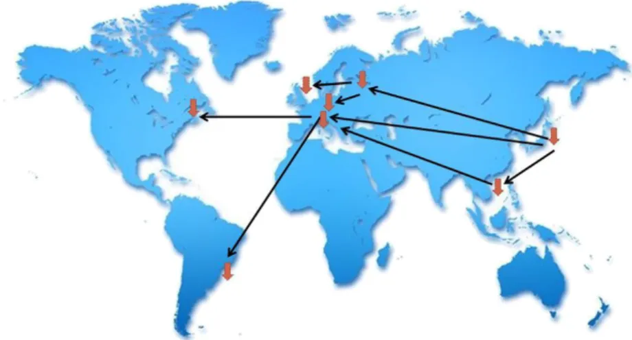
80
a private belief about the state of the world, and a social belief formed from observing the actions of
81
peers. They show how the probability that banks will synchronize their investment strategies
82
depends on the weighting between private and social belief.
83
84
In the following we will place the emphasis on the fact that price formation is the result of
85
human decision of buying or selling assets. Behind every trade is a human decision making, if not
86
by direct action of a human, then indirectly through the decision making made into the programs
87
that governs algorithmic trading made by computers. Socio-‐‑Finance [1] considers price formation as
88
a sociological phenomenon. It defines price formation to result from either direct or indirect human
89
interactions. Direct interaction covers the case where either individuals, or groups of individuals,
90
communicate directly and thereby influences mutual decision making with respect to trading
91
assets. At the first level, the individual level, indirect interaction covers the case where a trader
92
submits an order to buy or sell an asset. The resulting price movement of the asset is observed by
93
other traders, who in turn may change their decision making because of the price movement of the
94
asset caused by the initial trade. At the second level, the group level, indirect interaction covers the
95
case where whole markets have to wait on the outcome of pricing in other markets in order to find
96
the proper pricing.
97
98
2. Three different ways synchronization can lead to contagion in financial markets
99
2.1. Synchronization through indirect interaction of traders
100
This section is divided into two parts: indirect interaction of market participants at the individual
101
level (section 2.1.1) and indirect interaction of market participants at the collective level (section
102
2.1.2).
103
2.1.1. Synchronization through indirect interaction of individuals: the first level
104
The deed of traders in the past, has a direct influence of the action of traders at the present. Past
105
buying and selling activities has led the market up to the present level, for which traders have to
106
decide whether now is an opportune moment to buy or sell. This applies to traders using technical
107
analysis, as well as traders instead using fundamental analysis. Technical analysis will give
108
different buy/sell signals depending on the exact price history made by traders in the past, whereas
109
fundamental analysis will make traders judge about whether the price level has become sufficient
110
low in order to buy, or high enough in order to sell.
111
So, as traders take note of what happens in the market, and update their trading strategies
112
accordingly, the new evaluations of their strategies will change their future prospects of how to
113
trade in the market. Therefore as the markets change, the decision making of traders with respect to
114
buying/selling change, and as they change, they thereby change the pricing of the market. This
115
feedback loop is illustrated schematically in the figure below.
116
117
Figure 1. Representation of the price dynamics in the Minority-‐‑Game [12] and the $-‐‑Game [13].
118
Agents first update scores of all their strategies depending on their ability to predict the market
119
movement. After scores have been updated, each agent chooses the strategy which now has the
120
highest score. Depending on the price history at that moment, this strategy determines which action
121
a given agent will take. Finally, the sum of the actions of all agents determines the next price move:
122
if positive, the price moves up, if negative, the price moves down. The figure is taken from [14].
123
124
Under certain circumstances it can happen that traders inadvertently ends up in a state where their
125
trading strategies “decouple” from the price history, so that over the next (evt. few) time step(s)
126
their decision making become completely deterministic, independent of what happens next in the
127
market. In order to illustrate this point, consider the table below which is one way of formalizing
128
technical analysis trading strategies in a simple table form [12,13]. Considering for simplicity only
129
the direction of each of the last market moves, the table below predicts, for each possible price
130
history, the next move of the market. The table illustrates one technical analysis strategy that uses
131
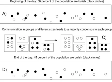
the last three time periods in providing a prediction, and can easily be generalized to any number
132
of periods.
133
134
Table 1. Example of a strategy used in the Minority Game[12] and the $-‐‑Game[13]. Considering
135
only up (1) and down (0) price movements of the market, a strategy issues a prediction for each
136
given price history, here illustrated with price histories over the last m=3 days.
137
138
price history prediction 0 0 0 1 0 0 1 -‐‑1 0 1 0 1 0 1 1 1 1 0 0 -‐‑1 1 0 1 -‐‑1 1 1 0 1 1 1 1 1
139
Consider now a given price history of the market, 𝜇(𝑡) = (010), at time t, meaning that (as
140
illustrated in the figure below) three time periods ago the market went down, then up, and then
141
down. It should now be noted that whatever the price movement at the next time period t+1, the
142
strategy in table 1 will always predict to sell at time period t+2. Therefore we don’t need to wait for
143
the market outcome at the next time step t+1 in order to know what the strategy will suggest
144
following that time step: it will always suggest selling at time t+2. That such kinds of dynamics in
145
the decision making of technical analysis strategies could be relevant for real market was suggested
146
in [15]. In the terminology of [15] the strategy in table 1 is called “one time step decoupled
147
conditioned on the price history 𝜇 = (010) ” and denoted 𝑎!!"#$%&'"!(𝑡).
We can then divide trading strategies into two different classes: those coupled to the price history
149
(i.e. conditioned on knowing 𝜇(𝑡) one cannot know the prediction of 𝑎!!"#$%&'(𝑡) at time t+2 before
150
knowing 𝜇(𝑡 + 1)), and those decoupled to the price history. Considering only the strategies
151
actually used by the agents to trade at time t, the order imbalance, A(t), can therefore be written:
152
𝐴 𝑡 ≡ 𝐴!!"#$%&' 𝑡 + 𝐴!!"#$%&'"!(𝑡) (1)
153
With 𝐴!!"#$%&' 𝑡 = 𝑎!!"#$%&'(𝑡) the sum over coupled strategies at time t and similarly for
154
𝐴!!"#$%&'"! 𝑡 = 𝑎!!"#$%&'"!(𝑡). The condition for certain predictability at time t, two time steps
155
ahead is then:
156
𝐴!!"#$%&'"! 𝑡 + 2 > 𝑁/2. (2)
157
If a majority of market participants hold decoupled strategies, this will ensure a deterministic future
158
price movement of the market, independent of the choices made the minority that hold coupled
159
strategies.160
161
162
Figure 2. Representation of how the trading strategy in Table1 decouples at time t+2 conditioned on
163
the price history 𝜇 = 010 at time t. Figure taken from [14].
164
The condition (2) gives the condition for synchronization to happen via indirect interaction of
165
traders through the price formation of an asset. Before considering synchronization in real markets
166
[14], one obviously first have to show its presence in models as well as in experiments. Indeed,
167
Figure 3 below proves synchronization via decoupling to be present in models like the Minority
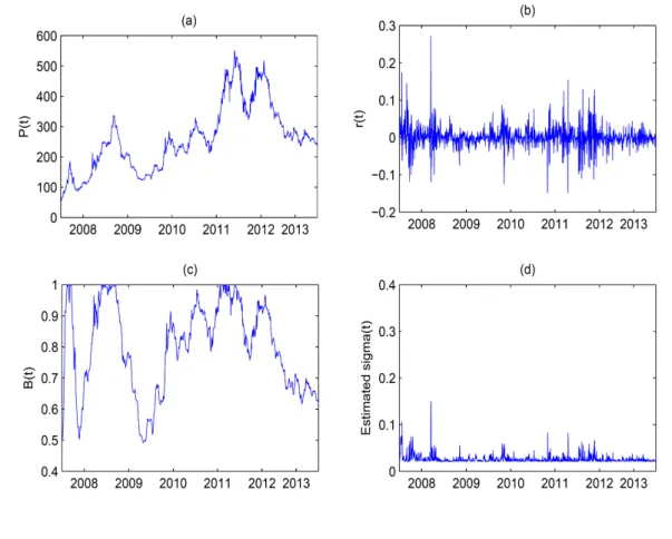
168
Game, a somewhat surprising result since these types of games by definition don’t support trend
169
following strategies. For more literature covering the situation with respect to synchronization in
170
experiments and markets, see [14-‐‑16].
171
172
173
174
Figure 3. An example of 𝐴!"#$%&'"! defined from (1) as a function of time for a simulation of the
175
Minority Game. Circles indicate one-‐‑step days which are predictive with probability 1, crosses are
176
the subset of days starting a run of two or more consecutive on-‐‑step predictive days.
177
178
2.1.2. Synchronization through indirect interaction of groups of individuals: the second level
179
Having discussed how indirect interaction of individuals through financial indices can lead to
180
synchronization, let us next consider how the phenomenon can appear through indirect interaction
181
of groups of individuals. In this case we consider the reaction of one market to the pricing created
182
in another market. That is, we consider how one given market (i.e. a pool of traders) reacts to prior
183
price formation in another market (created by another pool of traders).
184
To illustrate this point, consider the figure below which shows how large price movements of large
185
capital stock indices, can have a particular impact on smaller capital stock indices. The figure
186
illustrates the effect of both a world market return (calculated as a weighted sum of returns of stock
187
indices) and the US market return on the following price movements of individual stock indices.
188
Using the open-‐‑close return of the U.S. stock market, gives a particular clear case to see a ‘‘large-‐‑
189
move’’ impact across markets: since the Asian markets close before the opening of the U.S. markets,
190
they should only be able to price in this information at their opening the following day. That is, one
191
can consider the impact in the ‘‘close-‐‑open’’ of the Asian markets that should follow after an ‘‘open-‐‑
192
close’’ of the US market. An eventual ‘‘large-‐‑move’’ U.S. open-‐‑close should therefore have a clear
193
impact on the following close-‐‑open of the Asian markets. From the figure below this is indeed seen
194
to be the case. On the contrary, the European markets are still open when the U.S. market opens up
195
in the morning, so the European markets have access to part of the history of the open-‐‑close of the
196
U.S. markets. An eventual ‘‘large-‐‑move’’ U.S. open-‐‑close would therefore still be expected to have
197
an impact on the following close-‐‑open of the European markets, but with larger variation in the
198
response than for the Asian markets, since part of the U.S. move would already be priced in when
199
the European markets closed. This is seen to be the case.
200
201
202
203
Figure 4. Illustration of change blindness: a large world market return (fig a) or US market return
204
(fig b) impacts a given stock exchange, whereas small returns have random impact. a) Conditional
205
probability that the daily return Ri of a given country’s stock market index has the same sign as the
206
world market return. b) Conditional probability that the close-‐‑open (+: European markets; circles:
207
Asian markets) return Ri of a given country’s stock market index following an U.S. open-‐‑close, has
208
the same sign as the U.S. open-‐‑close return. The figures were created using almost 9 years of daily
209
returns of 24 of the major stock markets worldwide. For more information see [17-‐‑18]
210
211
To see how synchronization can happen across markets, consider the illustration in Figure 4.a
212
below which shows three Integrate-‐‑And-‐‑Fire (IAF) oscillators with the same frequency over one
213
time period (or equivalently one IAF oscillator over three time periods). An IAF oscillator is
214
characterized by an accumulation (i.e. “Integrate”) in amplitude A(t) (e.g. “stress”) over time t, up
215
to a certain point 𝐴!, after which it discharges (i.e. “Fires”). The complexity of models of IAF
216
oscillators arise when the oscillators are coupled (i.e. the amplitude of one oscillator influences the
217
amplitude of other oscillators), and have different frequency (see Figure 4.b) and/or thresholds 𝐴!!.
218
Peskin [19] introduced IAF oscillators in neurobiology to describe the interactions of neurons, but
219
IAF oscillators have been introduced in many other contexts, for network studies of IAF oscillators
220
see e.g. Mirollo and Strogatz [20], Kuramoto [21], Bottani [22]. The link between certain, types of
221
integrate-‐‑and-‐‑fire oscillators are earthquake models has also been noted by e.g. Corral et al. [23].
222
As mentioned in [17], one can consider each financial market index as an IAF oscillator that
223
influences other market indices (i.e. other IAF oscillators). The impact, or “stress”, from index i on
224
index j accumulates up to a certain point, after which it becomes priced-‐‑in. The justification for such
225
a behavior, can be seen from Figure 4, which shows that small price changes of index i has no
226
immediate influence on index j (but is assumed to accumulate over time), whereas large price
227
changes at index i, have an impact and thereby becomes priced-‐‑in at index j.
228
229
230
231
Figure 5. Illustration of an IAF oscillator. a) Illustrates the case where the amplitude A(t) of an IAF
232
oscillator integrates linearly in time until it reaches a critical value Ac, after which it discharges by
233
setting A(t) = 0. The case in a) can be viewed as one IAF oscillating over three periods of time, or
234
equivalently, three identical and uncoupled IAF oscillators oscillating over one period of time. b)
235
An IAF oscillator with random frequency over three time periods, or equivalently, three different
236
unit oscillators with random frequency over one time period. The figure is taken from [18].
237
238
239
This can be formalized in the following expression which expresses the set of stock market indices
240
worldwide as a set of coupled IAF oscillators:
241
𝑅! 𝑡 = !! ! ∗ !!!!𝛼!"𝜃 𝑅!"!"# (𝑡 − 1) > 𝑅! × 𝑅!"!"# 𝑡 − 1 𝛽!"+ 𝜑!"(𝑡) (3)242
𝑅!"!"# 𝑡 = [1 − 𝜃 𝑅 !"!"# 𝑡 − 1 > 𝑅! ] × 𝑅!"!"#(t-‐‑1) + 𝑅!(𝑡), 𝑗 ≠ 𝑖 (4)243
𝛼!" = 1 -‐‑ exp [−𝐾!/(𝐾! 𝛾) ] ; 𝛽!" = exp − 𝑧!− 𝑧!|/𝜏 ] (5)244
In expression (3) 𝑅!(t) is the return of stock index j, which at time t receives a contribution from
245
stock index j, whenever the “stress” 𝑅!"!"# exceeds a certain threshold 𝑅!. 𝛼!" describes the coupling
246
between the two stock indices, expressed via (5) in terms of the relative weight of capitalizations 𝐾!.
247
A large 𝛾, 𝛾 ≫ 1, corresponds to a network of the world’s indices with dominance of the index with
248
the largest capitalization Kmax. On the contrary a small 𝛾, 𝛾 ≪ 1, corresponds to a network of
249
indices with equal strengths since 𝛼!" then becomes independent of i, j. In addition it is assumed
250
that countries which are geographically close, also have larger interdependence economically, as
251
described by the coefficient 𝛽!", with | 𝑧!− 𝑧 ! | the time zone difference of countries i,j. 𝜏 gives the
252
scale over which this interdependence declines. Small 𝜏, 𝜏 ≪ 1, then corresponds to a world where
253
only indices in the same time zone are relevant for the pricing, whereas large 𝜏, 𝜏 ≫ 1, describes a
254
global influence in the pricing independent of the difference in time zone.
255
It is seen from (4), that it is the tensor 𝑅!"!"#, that places the role of an IAF oscillator. Returns from
256
index j, 𝑅!, accumulates stress on index i by continuously adding to 𝑅!"!"#, up to a certain point,
257
𝑅!"!"# > 𝑅!, after which the oscillator discharges, 𝑅!"!"# → 0, and the stress becomes priced-‐‑in via
258
(3).259
Once the IAF network is in a state of synchronization, it is possible to identify contagion effects
260
throughout the network. One example is given in Figure 5 below, showing the propagation of a
261
large price movement taking place in the Japanese stock market on the 23/05/2013. For more
262
examples on real market data see [18]
263
264
265
266
Figure 5. “Price-‐‑quake”. One of the main advantages of the non-‐‑linearity in the integrate-‐‑and-‐‑fire
267
oscillator model is that it enables a clear-‐‑cut identification of cause and effect; The figure shows one
268
example of a price-‐‑quake, following an initial minus 7% price movement on the Japanese stock
269
market on 23/05/2013. The figure is taken from [18].
270
271
2.2. Synchronization through direct interaction of traders
272
2.2.1. Synchronization through direct interaction of individuals and groups of individuals: the first
273
and second level.
274
Having discussed how synchronization can immerge through indirect interaction through financial
275
market indices of individuals, or groups of individuals, we now instead consider the case of direct
276
interaction, that is, how decision making is influenced by direct communication between people or
277
groups of people. The idea is to see how discussions among market participants, can influence their
278
decision making with respect to buying/selling assets, which in turn can influence the market
279
performance. On the other hand, we will show how the market performance itself can be a relevant
280
factor in the process of decision making, thereby creating another feedback loop between the
281
decision making of people and market performance.
282
283
To see how this can take place consider Figure 6.a below, which illustrate a population of market
284
participants with different views of the market, which we for simplicity will take either to be
285
positive, bullish, or negative, bearish. Figure 6.a illustrates an example where initially half the
286
population is bearish, the other half bullish. One could for example imagine a morning meeting
287
taking place in a major bank or brokerage house, and so at the beginning of the day, we let people
288
meet and discuss around tables in groups of different sizes Figure 6.b. To illustrate how
289
communication between people can influence their decision making, consider first the simple case
290
where consensus making is determined by the majority opinion Figure 6.c. As seen in Figure 6.d, at
291
the end of the day the opinion of the population has changed as a result of their meetings (direct
292
interaction), with now only 45% of the population being bullish.
293
294
Figure 6. Changing the “bullishness” in a population via communications in subgroups. (a) At the
295
beginning of a given day t a certain percentage B(t) of bullishness. (b) During the day
296
communication takes place in random subgroups of different sizes. Panel (c) illustrates the extreme
297
case of complete polarization mk,j = ±1 created by a majority rule in opinion. In general mk,j ≃ j/k
298
corresponds to the neutral case where in average the opinion remains unchanged within a subgroup
of size k. (d) Due to the communication in different subgroups the “bullishness” at the end of the
300
day is different from the beginning of the day. The figure is taken from [25].
301
302
In the context of decision making with respect to trading assets in financial markets, it is natural to
303
assume that the market performance itself could influence the decision making of the market
304
participants, whereas this in turn could influence future market performance. In order to capture
305
such kinds of feedbacks, a model was suggested in [25]. The main idea is to let the market
306
performance influence the decision making, instead of the simple majority rule seen in Figure 6.b-‐‑c.
307
This is done by assuming a certain probability for a majority opinion to prevail. Thereby under
308
certain conditions, a minority could persuade a part of the majority to change their opinion. The
309
probability for a majority opinion to prevail, will depend on the market performance over the last
310
time period.
311
Specifically, let B(t) denote the proportion of bullishness in a population at time t, the proportion of
312
bearishness is then 1 − B(t). For a given group of size k with j agents having a bullish opinion and k
313
− j a bearish opinion, we let m!,! denote the transition probability for all (k) members to adopt the
314
bullish opinion, as a result of their meeting. After one update taking into account communications
315
in all groups of size k with j bullish agents, the new probability of finding an agent with a bullish
316
view in the population can therefore be written:
317
𝐁 𝐭 + 𝟏 = 𝐦𝐤𝐣 𝐭 𝐂𝐣𝐤𝐁𝐣[𝟏 − 𝐁(𝐭)]𝐤!𝐣 (6)318
with319
𝐂𝐣𝐤 ≡ 𝐤! 𝐣! 𝐤!𝐣 ! (7)320
It should be noted that the transition probabilities 𝐦𝐤,𝐣(t) depend on time, since we assume that they
321
change as the market performance changes.
322
The link between communication and its impact on the markets, can now be taken into account by
323
assuming that the price return r(t) changes whenever there is a change in the bullishness. It should
324
now be noted, that it is the changes in opinion that matters for the market performance, rather than
325
the level of a given opinion. Empirical data supporting this idea, can for example be found in [26].
326
The reasoning behind this, is that people having a positive view of the market would naturally
327
already hold long positions on the market. It is therefore rather when people change their opinion,
328
say becoming more negative about the market, or less bullish, that they will have the tendency to
329
sell. Assuming the return to be proportional to the percentage change in bullishness, RB(t), as well
330
as economic news, 𝝋(𝒕), the return r(t) is given by
331
𝒓 𝒕 = 𝑹𝑩(𝒕)𝝁 + 𝝋 𝒕 , 𝝁 > 𝟎 (7)
332
Here 𝝋(𝒕) is a Gaussian distributed variable with mean 0 that described a standard deviation that
333
varies as a function of time depending on changes in sentiment:
334
𝝈 𝒕 = 𝝈𝟎𝐞𝐱𝐩 𝑹𝑩 𝒕
𝜷 , 𝝈𝟎> 𝟎, 𝜷 > 𝟎. (8)
335
The impact from the market performance on the decision making, can then be taking into account
336
by letting 𝐦𝐤,𝐣 𝐭 depend on the market performance via:
337
𝒎𝒌,𝒋 𝒕 = 𝒎𝒌,𝒋 𝒕 𝐞𝐱𝐩 𝒓 𝒕
𝜶 , 𝜶 > 𝟎, 𝒎𝒌𝒋 ≤ 𝟏 (9)
338
In this way the transition probabilities for a change of opinion, (9), depend directly on the market
339
return over the last time period. The reasoning for such dependence, is that if for example the
340
market had a dramatic downturn at the close yesterday, then in meetings the next morning, those
341
with a bearish view will be more likely to convince even a bullish majority about their point of
342
view.
343
Synchronization in the decision making due to communication between people, can now be studied
344
via for example tipping point analysis. Once extreme sentiment, B=0,1, has been created via
345
synchronization, this can be used to identify a tipping point of the market: when say 𝐁 → 𝟏 any
346
further increase in B is limited, which in turn limits further price increases in the market. However,
347
any negative economic news, 𝝋(𝒕), will then lead to a decrease in B(t) through (7) and (9). The cases
348
of B=0,1 therefore acts as reflection points of the model, enabling thereby an identification of tipping
349
points of the price dynamics of the markets. One illustration of such tipping point dynamics in real
350
markets, can be seen in the figure below taken from [27]. In [27] maximum likelihood methods were
351
used to estimate the parameters of the model, after which an out-‐‑of-‐‑sample analysis was performed
352
on EUBanks index around the time of the financial crisis in 2008. As can be seen from Figure 7.a,c
353
prior peeks, 𝑩 ≅ 𝟏, in the estimated sentiment indeed announce a tipping point in the performance
354
of the return of the index.
355
356
358
359
360
361
Figure 7. This figure presents EUBanks index prices and returns, as well as the corresponding
362
estimated conditional volatilities and bullishness proportions under the assumption of conditional
363
Student-‐‑t distribution. (a) EUBanks index price P(t), (b) EUBanks index returns r(t), (c) Estimated
364
bullishness proportions B(t), (d) Estimated conditional volatilities σ(t). The figure is taken from [27]
365
366
367
3. Discussion368
We have introduce three different models from Socio-‐‑Finance in order to capture three
369
different pathways in which the market participants in financial markets could synchronize in
370
decision making, and thereby create the route to contagious and volatile market phases. One
371
pathway is caused when stock market indices, seen as a set of coupled integrate-‐‑and-‐‑fire oscillators,
372
synchronize in frequency. Another pathway happens due to feedback mechanisms between market
373
performance, and the use certain (decoupled) trading strategies. Finally a third pathway could take
374
place because of communication and its impact on human decision making.
375
Synchronization is a well know phenomenon used in economics, to describe how trading
376
partners can introduce synchronization in business cycles across international borders. With the
377
recent global financial crisis, one question is to what role financial market integration could have on
378
synchronization of business cycles across borders? Another question is whether synchronization
379
created endogenously in financial markets could spill over into the economy and thereby cause
380
synchronization in business cycles across borders? It should be noted, that very little research has
381
been done on synchronization that is created endogenously by the financial markets themselves,
382
without necessarily an economic cause. It is the hope of the authors that the preset article could
383
help fuel awareness and interest on the topic.
384
385
Acknowledgments: This work was achieved through the Laboratory of Excellence on Financial Regulation
386
(Labex ReFi) supported by PRES heSam under the reference ANR-‐‑10-‐‑LABX-‐‑0095. It benefitted from a French
387
government support managed by the National Research Agency (ANR) within the project Investissements
388
d’Avenir Paris Nouveaux Mondes (invesments for the future Paris-‐‑New Worlds) under the reference ANR-‐‑11-‐‑
389
IDEX-‐‑0006-‐‑02.
390
References
392
393
1. Vitting Andersen J.; Nowak A., An Introduction to Socio-‐‑Finance, Springer, Berlin, Germany 2013.
394
2. Dées S.; Zorell N.; Business Cycle Synchronization, Disentangling Trade and Financial Linkages. ECB
395
working paper series 2011 no. 1322
396
3. Frankel, J. A.; Rose A. K. The Endogeneity of the Optimum Currency Area Criteria. Economic Journal 1998,
397
108(449), 1009-‐‑25.
398
4. Baxter, M.; Kouparitsas M. A. Determinants of business cycle co-‐‑movement: a robust analysis. Journal of
399
Monetary Economics 2005, 52(1), 113-‐‑157.
400
5. Backus, D. K.; Kehoe P. J.; Kydland F. E. International Real Business Cycles. Journal of Political Economy
401
1992, 100(4), 745-‐‑75.
402
6. Rey H. Dilemma not Trilemma: The global Financial Cycle and Monetary Policy Independence. NBER
403
Working Paper 2015 No. 21162
404
7. Poledna S.; Thurner S.; Farmer J. D.; Geanakoplos J. Leverage-‐‑induced systemic risk under Basle II and
405
other credit risk policies. Journal of Banking & Finance 2014, 42, 199–212.
406
8. Aymanns, C.; Georg, C-‐‑P. Contagious synchronization and endogenous network formation in financial
407
networks. Journal of Banking & Finance 2015, 50, 273–285.
408
9. Devenow A.; Welch, I. Rational herding in financial economics. European Economic Review 1996 Vol. 40
409
Nos 3-‐‑5.
410
10. Spyrou S. Herding in financial markets: a review of the literature, Review of Behavioral Finance 2013, Vol. 5
411
Issue: 2, 175-‐‑194.
412
11. Keynes J. M. The General Theory of Employment, Interest and Money, Macmillan Publications London
413
UK 1936.
414
12. Challet D.; Zhang Y.-‐‑C. Emergence of cooperation and organization in an evolutionary game. Physica A
415
1997, 246, 407-‐‑418.
416
13. Andersen J. V.; Sornette D. The Dollar Game. Eur.Phys. J. B 2003 31, 141.
417
14. Liu Y.-‐‑F.; Andersen J. V.; de Peretti P. Onset of financial instability studied via agent-‐‑based models,
418
chapter in “Systemic Risk Tomography”, 2016 edited by M. Billio, L. Pelizzon and R. Savona , ISBN
419
9781785480850
420
15. Andersen J. V.; Sornette D. A mechanism for pockets of predictability in complex adaptive systems. Eur.
421
Phys. Lett. 2005, 70, 697-‐‑703.
422
16. Liu Y.-‐‑F.; Andersen J. V. ; Frolov M.; de Peretti P.; “Experimental determination of synchronization in
423
human decision-‐‑making”, preprint, submitted to American Economic Review (2017).
424
17. Andersen J. V; Nowak A.;, Rotundo G.;, Parrot L.; Martinez S.; “Price-‐‑Quakes” Shaking the World’s
425
Stock Exchanges. PLoS ONE 2011 6 (11): e26472. Doi:10.1371/journal.pone.002647.
426
18. Bellenzier L.; Andersen J. V.; Rotundo G. Contagion in the world’s stock exchanges seen as a set of
427
coupled oscillators. Econ. Mod. 59 2016, 59, 224–236.
428
19. Peskin C. S., Mathematical Aspects of Heart Physiology, Courant Institute of Mathematical Science, New
429
York University, New York, 1975.
430
20. Mirollo R. E.; Strogatz M. E. Synchronization of pulse-‐‑coupled biological oscillators. SIAM J. Appl. Math.
431
1990, 50, 1645-‐‑1662.
432
21. Kuramoto Y. Collective synchronization of pulse-‐‑coupled oscillators and excitable units. Phys. D 1991, 50,
433
15-‐‑30.
434
22. Bottani S. Pulse-‐‑coupled relaxation oscillators: From biological synchronization to self-‐‑ organized
435
criticality. Phys. Rev. Lett. 1995, 74, 4189-‐‑419.
436
23. Corral A.; Pérez C. J.; Díaz-‐‑Guilera A.; Arenas A. Self-‐‑Organized Criticality and Synchronization in a
437
Lattice Model of Integrate-‐‑and-‐‑Fire Oscillators. Phys. Rev. Lett. 1995, 74, 118.
438
24. Corral A.; Pérez C. J.; Díaz-‐‑Guilera A.; Arenas A. Self-‐‑Organized Criticality and Synchronization in a
439
Lattice Model of Integrate-‐‑and-‐‑Fire Oscillators. Phys. Rev. Lett. 1995, 74, 118.
440
25. Andersen J. V.; Vrontos I.; Dellaportas P.; Galam S.; Communication impacting financial markets. Eur.
441
Phys. Lett. 2014 108, 28007.
442
26. The Hulbert Stock Newsletter Sentiment Index (HSNSI) is used among practitioners as a contrarian signal
443
for future stock returns, see also http://www.cxoadvisory.com/3265/sentiment-‐‑indicators/mark-‐‑hulbert/.
444
27. Andersen J. V;, Vrontos I.; Dellaportas P.; A Socio-‐‑Finance Model: Inference and empirical application.
446
Syrto preprint, the article can be downloaded at the site http://syrtoproject.eu/wp-‐‑
447
content/uploads/2014/10/19 ATHENS3.pdf
448
28. Georg C.-‐‑P.; The effect of the interbank network structure on contagion and common shocks. Journal of
449
Banking & Finance 2013, 37, 2216–2228.
450
29.
![Figure 1. Representation of the price dynamics in the Minority-‐‑Game [12] and the $-‐‑Game [13]](https://thumb-eu.123doks.com/thumbv2/123doknet/13241801.395431/6.892.164.741.376.730/figure-representation-price-dynamics-minority-game-game.webp)
![Table 1. Example of a strategy used in the Minority Game[12] and the $-‐‑Game[13]](https://thumb-eu.123doks.com/thumbv2/123doknet/13241801.395431/7.892.340.554.384.827/table-example-strategy-used-minority-game-game.webp)