Robust supervised classification with mixture models: Learning from data with uncertain labels

HAL Id: hal-00325263

https://hal.archives-ouvertes.fr/hal-00325263v2

HAL is a multi-disciplinary open access

archive for the deposit and dissemination of sci-entific research documents, whether they are pub-lished or not. The documents may come from

L’archive ouverte pluridisciplinaire HAL, est destinée au dépôt et à la diffusion de documents scientifiques de niveau recherche, publiés ou non, émanant des établissements d’enseignement et de

Robust supervised classification with mixture models:

Learning from data with uncertain labels

Charles Bouveyron, Stephane Girard

To cite this version:

Charles Bouveyron, Stephane Girard. Robust supervised classification with mixture models: Learn-ing from data with uncertain labels. Pattern Recognition, Elsevier, 2009, 42 (11), pp.2649-2658. �10.1016/j.patcog.2009.03.027�. �hal-00325263v2�

Robust supervised classification with mixture models:

Learning from data with uncertain labels

Charles Bouveyron1

& Stéphane Girard2

1 _{SAMOS-MATISSE, CES, UMR CNRS 8174,} University Paris 1 (Panthéon-Sorbonne)

2 _{MISTIS, INRIA Rhône-Alpes & LJK}

Abstract

In the supervised classification framework, human supervision is required for labeling a set of learning data which are then used for building the classifier. However, in many applications, human supervision is either imprecise, diffi-cult or expensive. In this paper, the problem of learning a supervised multi-class multi-classifier from data with uncertain labels is considered and a model-based classification method is proposed to solve it. The idea of the proposed method is to confront an unsupervised modelling of the data with the super-vised information carried by the labels of the learning data in order to detect inconsistencies. The method is able afterward to build a robust classifier taking into account the detected inconsistencies into the labels. Experiments on artificial and real data are provided to highlight the main features of the proposed method as well as an application to object recognition under weak supervision.

Key words: supervised classification, data with uncertain labels, mixture

models, robustness, label noise, weakly-supervised classification. 1. Introduction

In the supervised classification framework, human supervision is required to associate labels with a set of learning observations in order to construct a classifier. However, in many applications, this kind of supervision is either imprecise, difficult or expensive. For instance, in bio-medical applications, domain experts are asked to manually label a sample of learning data (MRI images, DNA micro-array, ...) which are then used for building a super-vised classifier. The cost of the supervision phase is usually high due to the

difficulty of labeling complex data. Furthermore, an human error is always possible in such a difficult task and an error in the supervision phase could have big effects on the decision phase, particularly if the size of the learn-ing sample is small. It is therefore very important to provide supervised classifiers robust enough to deal with data with uncertain labels.

1.1. The label noise problem

In statistical learning, it is very common to assume that the data are noised. Two types of noise can be considered in supervised learning: the noise on the explanatory variables and the noise on the response variable. Noise on explanatory variables has been widely studied in the literature whereas the problem of noise on the response variable has received less attention in some supervised situations. While almost all approaches model the noise on the response variable in regression analysis (see Chap. 3 of [15] for details), label noise remains an important and unsolved problem in supervised clas-sification. Brodley and Friedl summarized in [7] the main reasons for which label noise can occur. Since the main assumption of supervised classification is that the labels of learning samples are true, existing methods giving a full confidence to the labels of the learning data naturally provide disappointing classification results when the learning dataset contains some wrong labels. Particularly, model-based discriminant analysis methods such as Linear Dis-criminant Analysis (LDA, see Chap. 3 of [21]) or Mixture DisDis-criminant Anal-ysis (MDA, see [14]) are sensitive to label noise. This sensitivity is mainly due to the fact that these methods estimate the model parameters from the learning data and label noise naturally perturbs these estimates.

1.2. Related works

Learning a supervised classifier from data with uncertain labels can be achieved using three main strategies: cleaning the data, using robust estima-tions of model parameters and finally modelling the label noise.

Data cleaning approaches. Early approaches tried to clean the data by

re-moving the misclassified instances using some kind of nearest neighbor al-gorithm [10, 12, 30]. Other works treat the noisy data using the C4.5 algo-rithm [17, 32], neural networks [31] or a saturation filter [11]. Hawkins et

al. [16] identified as outliers the data subset whose deletion leads to the

et al. proposed in [13] to remove noisy observations with a cumulative

infor-mation criterion and further checking by human experts. However, removing noisy instances could decrease the classification bias but also increase the classification variance since the cleaned dataset is of smaller size than the original one. Thus, this procedure could give a less efficient classifier than the classifier built with noisy data when the number of learning data is small.

Robust estimation of model parameters. Therefore, other researchers

pro-posed not to remove any learning instance and to build instead supervised classifiers robust to label noise. Bashir et al. [2] focused on robust esti-mation of the model parameters in the mixture model context. Maximum likelihood estimators of the mixture model parameters are replaced by the corresponding S-estimators (see Rousseeuw and Leroy [25] for a general ac-count on robust estimation) but the authors only observed a slight reduction of the average probability of misclassification. Similarly, Mingers [23], Sakak-ibara [26] and Vannoorenberghe et al. [29] proposed noise-tolerant approaches to make decision tree classifiers robust to label noise. Boosting [24, 27] can also be used to limit the sensitivity of the built classifier to the label noise.

Noise modelling. Among all these solutions, the model proposed in [18] by

Lawrence et al. has the advantage of explicitely including the label noise in the model with a sound theoretical foundation in the binary classifica-tion case. Denoting by y and ˜y the actual and the observed class labels of an observation x, it is assumed that their joint distribution can be fac-torised as p(x, y, ˜y) = P (y|˜y)p(x|y)P (˜y). The class conditional densities p(x|y) are modelled by Gaussian distributions while the probabilistic rela-tionship P (y|˜y) between noisy and observed class labels is specified by a 2 × 2 probability table. An EM-like algorithm is introduced for building a kernel Fisher discriminant classifier on the basis of the above model. This work was recently extended by Li et al. in [19] who proposed a new in-corporation of the noise model in the classifier and relaxed the distribution assumption of Lawrence et al. by allowing each class density p(x|y) to be modeled by a mixture of several Gaussians.

1.3. The proposed approach

We propose in this paper a supervised classification method, called Ro-bust Mixture Discriminant Analysis (RMDA), designed for dealing with la-bel noised data. Conversely to the noise modelling methods, the approach

proposed in this paper does not rely on a specific label noise model which could be ill adapted in some situations. The main idea of our approach is to compare the supervised information given by the learning data with an unsupervised modelling based on the Gaussian mixture model. With such an approach, if some learning data have wrong labels, the comparison of the supervised information with an unsupervised modelling of the data allows to detect the inconsistent labels. It is possible afterward to build a supervised classifier by giving a low confidence to the learning observations with incon-sistent labels. The main advantages of the proposed approach compared to previous works are the explicit modelling of more than two classes and the flexibility of the method due to the use of a global mixture model.

The remainder of this paper is organized as follows. The model of the proposed method is presented in Section 2 and Section 3 is devoted to the inference aspects. Experimental studies on simulated and real datasets are reported in Section 4. Finally, an application to object recognition under weak supervision is presented in Section 5.

2. Robust mixture discriminant analysis

In order to compare the supervised information given by the learning data with an unsupervised modelling, we propose to use an unsupervised mixture model in which the supervised information is introduced.

2.1. The mixture model

Let us consider a mixture model in which two different structures coexist: an unsupervised structure of K clusters (represented by the random discrete variable S) and a supervised structure, provided by the learning data, of k classes (represented by the random discrete variable C). As in the stan-dard mixture model, we assume that the data (x1, ..., xn) are independent

realizations of a random vector X ∈ Rp _{with density function:}

p(x) =

K

X

j=1

P (S = j)p(x|S = j), (1)

where P (S = j) is the prior probability of the jth cluster and p(x|S = j) is the corresponding conditional density. Let us now introduce the supervised

information carried by the learning data. Since Pk

i=1P (C = i|S = j) = 1

for all j = 1, ..., K, we can plug this quantity in (1) to obtain: p(x) = k X i=1 K X j=1 P (C = i|S = j)P (S = j)p(x|S = j), (2)

where P (C = i|S = j) can be interpreted as the probability that the jth clus-ter belongs to the ith class and thus measures the consistency between classes and clusters. Using the classical notations of parametric mixture models and introducing the notation rij = P (C = i|S = j), we can reformulate (2) as

follows: p(x) = k X i=1 K X j=1 rijπjp(x|S = j), (3)

where πj = P (S = j). Therefore, (3) exhibits both the “modelling” part

of our approach, based on the mixture model, and the “supervision” part through the parameters rij. Since the modelling introduced in this section

is based on the mixture model, we can use any conditional density to model each cluster. In particular, the use of the Gaussian mixture model is discussed below.

2.2. The case of Gaussian mixture models

Among all parametric densities, the Gaussian model is probably the most used in classification. The Gaussian mixture model has been studied exten-sively in the last decades and used in many situations (see [1] for a review).

Usual Gaussian model. In the case of the usual Gaussian mixture model, the

conditional density p(x|S = j) is modelled by a Gaussian density φ with mean µj and covariance Σj. Under this assumption, (3) can therefore be

rewritten as: p(x) = k X i=1 K X j=1 rijπjφ(x; µj, Σj). (4)

Parsimonious Gaussian models. In some situations, modelling the data with

a full covariance matrix can be too expensive in terms of number of parame-ters to estimate. In such a case, it is possible to make additional assumptions on the structure of the covariance matrix. For example, in the well-known Linear Discriminant Analysis (LDA) method, the covariance matrices of the

different components are supposed to be equal to a unique covariance matrix (common Gaussian model hereafter). It is also possible to assume that the covariance matrix of each mixture component is diagonal (diagonal Gaussian model) or proportional to the identity matrix (spherical Gaussian model). These models are known as parsimonious Gaussian models in the literature since they require to estimate less parameters than the classical Gaussian model. Celeux and Govaert proposed in [8] a family of parsimonious Gaus-sian models based on an eigenvalue decomposition of the covariance matrix including the previous models. These parsimonious Gaussian models were then applied in [4] to supervised classification.

Gaussian models for high-dimensional data. Nowadays, many scientific

do-mains produce high-dimensional data like medical research (DNA micro-arrays) or image analysis (see Section 5 for an illustration). Classifying such data is a challenging problem since the performance of classifiers suf-fers from the curse of dimensionality [3]. Classification methods based on Gaussian mixture models are directly penalized by the fact that the num-ber of parameters to estimate grows up with the square of the dimension. It is then necessary to use parsimonious Gaussian models in order to ob-tain stable classifier. However, these parsimonious models are usually too constrained to correctly fit the data in a high-dimensional space. To over-come this problem, Bouveyron et al. proposed recently in [5] a family of Gaussian models adapted to high-dimensional data. This approach, based on the idea that high-dimensional data live in low-dimensional spaces, as-sumes that the covariance matrix of each mixture component has only dj+ 1

different eigenvalues where dj is the dimension of the subspace of the jth

mixture component. This specific modelling allows to deal with the situa-tion where the class manifold and the data density could be not correlated in high-dimensional spaces.

2.3. Link with Mixture Discriminant Analysis

It is possible to establish a link between model (4) and the supervised method Mixture Discriminant Analysis (MDA) [14] in which each class is modelled by a mixture of Ki Gaussian densities. Denoting by K =Pki=1Ki

the total number of Gaussian components and keeping in mind the notations of Paragraph 2.1, MDA assumes that the conditional density of the ith class,

i = 1, ..., k, is: p(x|C = i) = K X j=1 πijφ(x; µj, Σj), (5)

where πij = P (C = i, S = j) is the prior probability of the jth mixture

component of the ith class. Note that πij = 0 if the jth mixture component

is not included in the ith class. Moreover, remarking that πij = rijπj, we

obtain p(x) = k X i=1 K X j=1 rijπjφ(x; µj, Σj), (6)

which formally corresponds to model (4). The main difference is that, in the MDA case, the labels are certain (supervised context). Thus, rij = P (C =

i|S = j) is known and reduces to rij = 1 if the jth mixture component

belongs to the ith class and rij = 0 otherwise. Consequently, in the case

where the labels of learning data are all consistent with the modelling of these data, RMDA should provide the same classifier as MDA.

2.4. Classification step

In model-based discriminant analysis, new observations are usually as-signed to a class using the maximum a posteriori (MAP) rule. The MAP rule assigns a new observation x to the class for which x has the highest posterior probability. Therefore, the classification step mainly consists in calculating the posterior probability P (C = i|X = x) for each class i = 1, ..., k. In the case of the model described in this section, this posterior probability can be expressed as follows using the Bayes’ rule:

P (C = i|X = x) =

K

X

j=1

rijP (S = j)p(x|S = j)/p(x),

and, since P (S = j|X = x) = P (S = j)p(x|S = j)/p(x), we finally obtain: P (C = i|X = x) =

K

X

j=1

rijP (S = j|X = x). (7)

Therefore, the classification step of RMDA relies on (7) and requires the estimation of the probabilities rij as well as the unsupervised classification

quantify the consistency between the groups and the classes, balance the importance of the groups in the final classification rule. Consequently, the classifier associated with this decision rule will be mainly based on the groups which are very likely to be made of points from a unique class.

3. Estimation procedure

Due to the nature of the model proposed in Section 2, the estimation pro-cedure is made of two steps corresponding respectively to the unsupervised and to the supervised part of the comparison. The first step consists in esti-mating the parameters of the mixture model in an unsupervised way leading to the clustering probabilities P (S = j|X = x). In the second step, the pa-rameters rij linking the mixture model with the information carried by the

labels of the learning data are estimated by maximization of the likelihood.

3.1. Estimation of the mixture parameters

In this first step of the estimation procedure, the labels of the data are discarded to form K homogeneous groups. Therefore, this step consists in estimating the parameters of the chosen mixture model.

Usual and parsimonious Gaussian models. In the case of the usual

Gaus-sian model, the classical procedure for estimating the proportions πj, the

means µj and the variance matrices Σj, for j = 1, ..., K, is the Maximum

Likelihood (ML) method. Unfortunately, it is not possible to find directly a solution of the maximum likelihood problem. In such a case, the Expectation-Maximization (EM) algorithm proposed by Dempster et al. (1977) provides the ML estimates of the parameters using an iterative procedure. We re-fer to [4] for the parameter estimation in the case of parsimonious Gaussian models.

Gaussian models for high-dimensional data. If the chosen mixture model

involves Gaussian models for high-dimensional data, this step consists in estimating the following model parameters: the proportions πj, the means

µj, the subspace variances (a1j, ..., adjj), the noise variance bj, the subspace

orientation matrix Qj and the subspace dimension dj for each mixture

com-ponent. In [5], an EM-like approach is presented to estimate the parameters πj, µj, aij, bj and Qj. An empirical strategy based on the eigenvalue scree

is also proposed in this work to find the intrinsic dimension of each mix-ture component. We refer to [5] for more details and to Section 5 for an application to object regognition.

3.2. Estimation of the parameters rij

In this second step of the procedure, the labels of the data are intro-duced to estimate the k × K matrix of parameters R = (rij) and we use

the parameters learned in the previous step as the mixture parameters. The parameters rij modify the unsupervised model for taking account of the label

information. They thus indicate the consistency of the unsupervised mod-elling of the data with the supervised information carried by the labels of the learning data. Since we consider a supervised problem, the labels c1, . . . , cn

of the learning data x1, . . . , x_n are known, and we can therefore introduce

Ci = {xℓ, ℓ = 1, . . . , n /cℓ = i}. From (7), the log-likelihood associated to our

model can be expressed as: ℓ(R) = k X i=1 X x∈Ci log P (X = x, C = i), = k X i=1 X x∈Ci log K X j=1 rijP (S = j|X = x) ! + ξ, where, in view of (1), ξ = Pk i=1 P

x∈Cilog p(x) does not depend on R. This

relation is matricially rewritten as: ℓ(R) = k X i=1 X x∈Ci log (RiΨ(x)) + ξ, (8)

with the RK_{-vector Ψ(x) = (P (S = 1|X = x), . . . , P (S = K|X = x))}t _and

where Ri is the ith row of R. Consequently, we end up with a constrained

optimization problem:      maximize Pk i=1 P x∈Cilog (RiΨ(x)) ,

with respect to rij ∈ [0, 1], ∀i = 1, . . . , k, ∀j = 1, . . . , K,

and Pk

i=1rij = 1, ∀j = 1, . . . , K.

Since it is not possible to find an explicit solution to this optimization prob-lem, an iterative optimization procedure has to be used to compute the max-imum likelihood estimators of the parameters rij. The partial derivatives

associated with (8) can be expressed as follows: ∂ℓ(R) ∂rij =X x∈Ci Ψj(x) RiΨ(x) ,

where Ψj(x) is the jth coordinate of Ψ(x). This optimum search has been

implemented in Matlab using the function fmincon which is designed to find a constrained optimum of multivariate functions.

3.3. Model selection and complexity

We now focus on the problem of choosing the most appropriate mixture model for RMDA. In the context of this work, this issue includes the selection of the conditional density of each mixture component as well as the choice of the number of sub-classes per mixture component. We discuss biefly as well the complexity and the scalability of RMDA.

Choosing a mixture model. As discussed in Paragraph 2.2, it is sometimes

useful to use a parsimonious model or a model designed for high-dimensional data depending on the nature of the data and the size of the training dataset. In order to choose among all existing models, it is possible to use either cross-validation or information criteria, such as the Bayesian Information Criterion (BIC) [28]. However, the practician has to be careful when choosing between both approaches. Indeed, choosing cross-validation implies that more importance is given to the labels of the learning dataset and this can be contrary to the idea that there is label noise in the data. On the other hand, adopting an information criterion, such as BIC, implies that more importance is given to the unsupervised modelling of the data.

Choosing the number of sub-classes. Selecting the number of sub-classes is

usually a complex problem since different classes can have a different num-ber of mixture components. For instance, in the case of MDA, trying out all combinations of component numbers will confront the practician to a compu-tational problem with a high level of complexity. In [14], the authors proposed to make the additional assumption that the numbers of mixture components of the classes are equal but this could be far away from the truth. Due to the nature of the RMDA model introduced in this paper, choosing the number of sub-classes per mixture component reduces to choosing the total number of clusters K. Indeed, the selection of the number of sub-classes per class

will be implicitely done through the parameters rij which measures the

con-sistency between the sub-classes and the mixture components. Therefore, it only remains to select the unique parameter K and this easier problem can be also addressed using cross-validation or BIC (with similar implications).

Complexity and scalability of RMDA. Regarding the model complexity, RMDA

mainly depends on the chosen mixture model since RMDA requires only to estimate the mixture parameters and the parameters rij. The number of

parameters rij to estimate is (k − 1)K and thus does not depend on the

dimension of the data. Conversely, the number of mixture parameters to estimate heavily depends on the data dimension. For instance, the num-ber of parameters to estimate in a Gaussian mixture of K classes in Rp _is

larger than Kp2

/2. Therefore, when the data dimension becomes high, it is preferable to switch for a parsimonious model which requires the estimation of less parameters. In particular, Gaussian models for high-dimensional data (see Paragraph 2.2) require only the estimation of approximatively Kpd/2 parameters, where d is the intrinsic data dimension. Therefore, these models are well suited for classifying high-dimensional data as soon as d is small compared to the original data dimension p. Regarding now the scalability, RMDA inherits its flexibility and its ability to model complex processes from MDA. This feature is mainly due to the modelling of each class by a mixture of several Gaussians in order to be able to deal with non-Gaussian data. 4. Experimental results

In this section, we present experimental results on artificial and real datasets in situations illustrating the problem of supervised classification under uncertainty.

4.1. Experimental setup

In the following studies, we consider the general problem of label switching between the classes. In this case, complex models are very sensitive but parsimonious models can also be affected if the contamination rate is high. In order to simulate a label noise, the observation labels have been switched following a Bernoulli distribution with parameter η ranging from 0 to 1 and representing the contamination rate. Each label ℓ is therefore left unchanged with probability 1 − η or switches to a value ℓ′

6= ℓ with probability η/k. In all studies, the performance of the methods is assessed by the correct

−3 −2 −1 0 1 2 3 4 −4 −3 −2 −1 0 1 2 −3 −2 −1 0 1 2 3 4 −4 −3 −2 −1 0 1 2

MDA with η = 0 RMDA with η = 0

−3 −2 −1 0 1 2 3 4 −4 −3 −2 −1 0 1 2 −3 −2 −1 0 1 2 3 4 −4 −3 −2 −1 0 1 2

MDA with η = 0.15 RMDA with η = 0.15

−3 −2 −1 0 1 2 3 4 −4 −3 −2 −1 0 1 2 −3 −2 −1 0 1 2 3 4 −4 −3 −2 −1 0 1 2

MDA with η = 0.30 RMDA with η = 0.30

−3 −2 −1 0 1 2 3 4 −4 −3 −2 −1 0 1 2 −3 −2 −1 0 1 2 3 4 −4 −3 −2 −1 0 1 2

MDA with η = 0.45 RMDA with η = 0.45

Figure 1: Decision rules for MDA and RMDA for increasing contamination rates η on a 2-dimensional simulated dataset (2 classes).

0 0.05 0.1 0.15 0.2 0.25 0.3 0.35 0.4 0.45 0.5 0.4 0.5 0.6 0.7 0.8 0.9 1 Contamination rate

Correct classification rate

LDA MDA RLDA RMDA

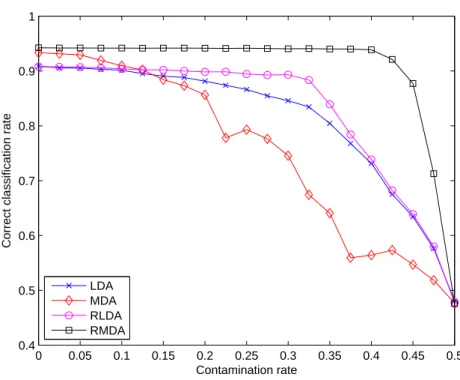
Figure 2: Performance of LDA, MDA, RLDA and RMDA for increasing contamination rates on a simulated dataset (2 classes).

classification rate and computed on a test dataset. The experiments have been repeated 25 times in order to average the classification results.

4.2. Binary classification (simulated data)

For this first experiment, we simulated the data following the mixture model of MDA and RMDA. The dataset is made of 2 classes and each class was modeled with a Gaussian mixture of 2 components. We used for the mix-ture components of each class a spherical Gaussian model. The means of the different mixture components were chosen in order to obtain two separated enough classes. Figure 1 compares the performance of MDA and RMDA (in-troduced in this paper) on a 2-dimensional simulated dataset for increasing contamination rates η. As expected, MDA and RMDA give similar decision rules when there is no label noise (η = 0). This observation confirms the existing link between both methods (see Paragraph 2.3). For higher con-tamination rates η, MDA builds very unstable decision rules whereas RMDA demonstrates its robustness by providing very stable decision boundaries.

Figure 3: Some examples of the USPS-24 dataset.

The performance of LDA, MDA, RLDA (proposed by Lawrence et al. (2001)) and RMDA on a 25-dimensional dataset simulated under similar conditions is illustrated on Figure 2. First, it appears that RMDA is as efficient as MDA when there is no label noise and this illustrates again the equivalence between both methods in this special case. On the one hand, LDA and MDA appear to be sensitive to contamination. Particularly, MDA becomes very unstable for contamination rates higher than 0.2. The behavior of these two supervised methods is not surprising since they both have full confidence in the labels of the data. On the other hand, RLDA turns out to be more robust than LDA but its performance quickly decreases for contamination rates higher than 0.3. Finally, RMDA appears to be particularly robust for a large panel of contamination rates (up to 0.4).

4.3. Binary classification (real data)

We consider here a dataset from the real world, called USPS-24, extracted from the well-known USPS dataset1_{. The learning dataset is made of 1383}

hand-written digits. Among them, 731 observations belong to the class of the digit 2 and of 652 observations belong to the class of the digit 4. Similarly, the test dataset contains 298 elements: 198 and 200 observations respectively from the classes of the digit 2 and 4. These two classes have been chosen since they have a high misclassification rate in the original USPS dataset. Each observation of the USPS-24 dataset corresponds to a 16 × 16 grey level image of a digit and represented as a 256-dimensional vector. Figure 3 shows some samples from the dataset. For both MDA and RMDA, each class was modeled by a mixture of 5 Gaussians and, due to the high dimension of the data, we used for each mixture component a spherical Gaussian model. Figure 4 shows the performance of LDA, MDA, RLDA and RMDA on the USPS-24 dataset for increasing contamination rates. As in the previous experiment,

0 0.05 0.1 0.15 0.2 0.25 0.3 0.35 0.4 0.45 0.5 0.4 0.5 0.6 0.7 0.8 0.9 1 Contamination rate

Correct classification rate

LDA MDA RLDA RMDA

Figure 4: Performance of LDA, MDA, RLDA and RMDA for increasing contamination rates on the USPS-24 dataset.

LDA and MDA appear to be very sensitive to contamination. RLDA is again more robust than LDA and MDA but its performance decreases quickly for contamination rates higher than 0.2. Finally, RMDA appears to be very robust for contamination rates up to 0.4 and to be almost as efficient as the other methods when the label noise is low. In this experiment, RMDA has therefore demonstrated its ability to deal with label noise in real and complex situations.

4.4. Multi-class classification (simulated data)

This last simulation study aims at demonstrating the ability of RMDA to deal with label noise in multi-class classification problem whereas the existing methods consider only binary classification. Indeed, the model of RLDA, proposed by Lawrence et al. [18] and its extension [19] are designed for only two classes. We therefore compare here RMDA to only LDA and MDA which are able to deal with multi-class classification problems as well. As before, we simulated the data following the mixture model of MDA and RMDA.

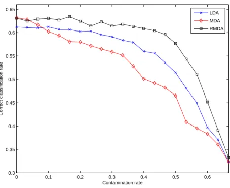
0 0.1 0.2 0.3 0.4 0.5 0.6 0.3 0.35 0.4 0.45 0.5 0.55 0.6 0.65 Contamination rate

Correct classification rate

LDA MDA RMDA

Figure 5: Performance of LDA, MDA and RMDA for increasing contamination rates on a simulated dataset (3 classes).

The simulated dataset is made of 3 classes and each class was modeled with a Gaussian mixture of 2 components in a 25-dimensional space. We used for the mixture components of each class a spherical Gaussian model. The means of the different mixture components were again chosen in order to obtain separated enough classes. Figure 5 shows the performance of LDA, MDA and RMDA for increasing contamination rates. Unsurprisingly, it can be noticed that the average correct classification rate of the methods is lower than in the binary classification case and decreases to 1/3. Secondly, it appears that RMDA is again as efficient as MDA when there is no label noise. Regarding the robustness of the studied methods, LDA and MDA have similar behaviours as in the binary case. The performance of MDA decreases almost linearly with the contamination rate. As in the previous experiments, LDA is more robust than MDA for low contamination rates but its performance decreases after 0.2. Finally, RMDA turns out to be as robust as in the binary case since its performance is almost constant for contamination rates up to 0.45. This experiment illustrates the robustness

of RMDA in the multi-class classification case which is a more common and difficult problem in practice than the binary classification problem.

5. Application to object recognition under weak supervision The supervised classification method proposed in this work is designed for performing classification in the presence of label noise. We present here an application of this method to object recognition under weak supervision.

5.1. Object recognition under weak supervision

Object recognition is one of the most challenging problems in computer vision and it requires that human experts segment a very large number of images for each object category. Earlier approaches characterized the objects by their global appearance and were not robust to occlusion, clutter and geometric transformations. To avoid these problems, recent methods use local image descriptors for selecting the relevant parts of the images and then classify these local descriptors to one of the object categories. Regarding the supervision, it is clear that it is impossible that human experts segment images for each object category given the infinite number of existing object categories. However, it is easy to obtain images containing a given object (using Google Image for instance) and to assume that all descriptors of these images are representative of the studied object even though we know that it is wrong. By doing that, we consciously introduce a label noise between the class “object” and the class “background” but, using the approach proposed in this paper, it should be possible to identify all pixels which actually belong to the class “object” and, finally, localize the studied object in the images. This approach will be called in the sequel weakly-supervised object recognition.

5.2. The data

The object category database used in this study is the Pascal dataset [9] which has been proposed for an object localization challenge organized by the Pascal Network. Examples of images in this dataset are presented in Figure 6. The Pascal dataset is divided into four categories: motorbikes, bi-cycles, people and cars. It contains 684 images for learning and two test sets:

test 1 (689 images) and test 2 (956 images). Images in test 1 were collected

from the same distribution as the training images. The set test 2 can be seen as a harder challenge since images are collected by “Google Image” and thus

L ea rn in g T es t 1 T es t 2

Bicycle Human Car Motorbike Figure 6: Some images used for learning and testing from the Pascal database [9].

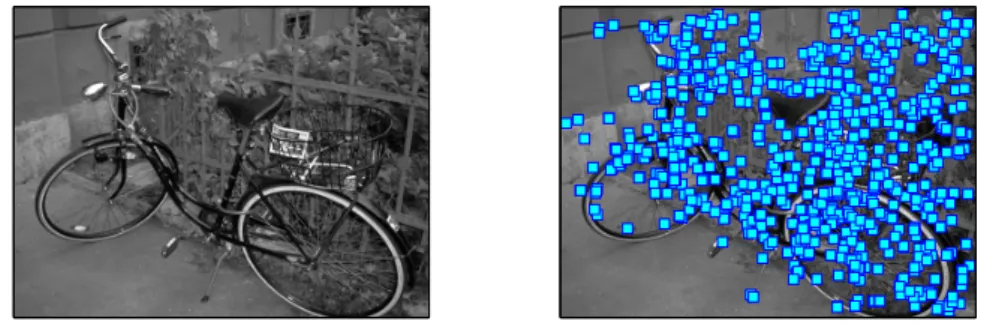
come from a different distribution than the training set. An additional diffi-culty for test 2 is that many images contain instances of several categories. The Pascal dataset also provides for each image a bounding box indicating the localization of the object. The local image descriptors were obtained by first using the Harris-Laplace detector [22] to extract interest points and by then using the SIFT descriptor [20] to represent the scale-invariant re-gions around these points. The dimension of the obtained SIFT features is 128. See [6] for more details on the image descriptor extraction. Therefore, the object recognition task reduces to classifying the detected interest points in a 128-dimensional space. We evaluated our approach in both supervised and weakly supervised frameworks. In the supervised framework, only the descriptors located inside the bounding boxes were labeled as belonging to the class “object” in the learning step. Conversely, in the weakly supervised framework, all descriptors of images containing at least one instance of the object were labeled as belonging to the class “object” for learning. Figure 7 shows on the left panel an original image and on the right panel all extracted interest points.

Figure 7: An original image from the Pascal test 1 dataset and the extracted interest points.

5.3. Experimental setup

We compared our approach based on RMDA with different Gaussian mod-els to the object localization methods of the Pascal Challenge [9]. For RMDA, we used parsimonious Gaussian models as well as Gaussian models for high-dimensional data, see Paragraph 2.2. On the one hand, we selected the following parsimonious Gaussian models: common covariance matrix Gaus-sian model (RMDA common), diagonal GausGaus-sian model (RMDA diagonal), spherical Gaussian model (RMDA spherical). On the other hand, the follow-ing Gaussian models for high-dimensional data were also selected: [aijbiQidi],

[aijbQidi], [aibiQidi], [aibQidi] and [aibiQid]. We refer to [5] for details on the

different models. For all the models the parameters were estimated via the EM algorithm using the same initialization. For high-dimensional models, the resulting average value for intrinsic dimensions di was approximately 10.

In this experiment, we used 50 clusters for modelling each of the four object categories whatever the clustering method used. In order to compare our results with the ones of the Pascal Challenge, we used the localization mea-sure “Average Precision” (AP) proposed for this competition. It quantifies the consistency between the interest points classified as “object” with the provided bounding boxes (see [9] for more details). Therefore, the higher the AP value is, the better the object localization is.

5.4. Experimental results

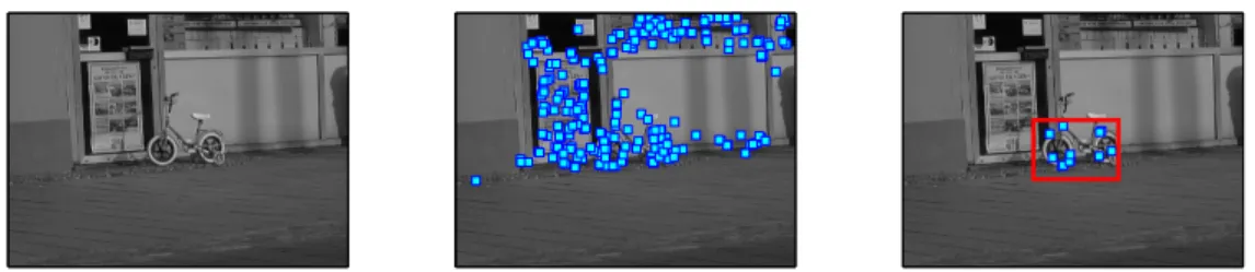
Figure 8 illustrates the localization process with our approach in the weakly-supervised framework on an image from the test 1 dataset. Table 1 summarizes the localization results obtained in the supervised and weakly-supervised frameworks with our approach on both Pascal test 1 and test 2

Figure 8: Weakly-supervised object localization on Pascal test 2 : An original image from the Pascal test 1 dataset (left), the extracted interest points (center) and the interest points classified as “object” with the provided bounding box (right).

and reports the results of the best method of the Pascal challenge. The values presented in this table are the mean of the AP measure obtained by the different methods over the 4 object categories (motorbikes, bicycles, peo-ple and cars). Detailed results are presented in the appendix. On the one hand, our approach performs well in the supervised case compared to the results obtained during the Pascal competition. Moreover, the models de-signed for high-dimensional data perform best among the different Gaussian mixture models. In particular, RMDA with high-dimensional models wins two “competitions” (bicycle and people) on Pascal test 1 (see Appendix A.1) and three “competitions” (motorbike, bicycle and people) on Pascal test 2 (see Appendix A.2). This is despite the fact that our approach assumes that there is only one object per image for each category and this reduces the performance when multiple objects are present. On the other hand, it appears that the results obtained in the weakly-supervised framework are not very different from those obtained in the supervised framework. This means that our approach efficiently identifies discriminative clusters of each object category and that even with a weak supervision. We do not have the corresponding results for the Pascal challenge methods since there was no competition for detection in the weakly-supervised framework. However, we can remark that RMDA performs best in the weakly-supervised framework compared to the results of the Pascal Challenge methods in the supervised framework.

These results are actually promising and mean that the weakly-supervised approach is tenable for object localization since the manual annotation of training images is time consuming. Furthermore, this study has shown that classification with label noise can be extended to classification under weak supervision and that RMDA is able to solve both problems in complex

situ-Database Pascal test 1 Pascal test 2

Supervision full weak full weak

RMDA [aijbiQidi] 0.302 0.273 0.172 0.145 RMDA [aijbQidi] 0.318 0.287 0.181 0.147 RMDA [aibiQidi] 0.313 0.285 0.183 0.142 RMDA [aibQidi] 0.318 0.283 0.176 0.148 RMDA [aibiQid] 0.314 0.287 0.179 0.130 RMDA spherical 0.271 0.216 0.149 0.106 RMDA diagonal 0.276 0.227 0.161 0.110 RMDA common 0.267 0.246 0.164 0.116 Best method of [9] 0.279 / 0.112 /

Table 1: Object localization results on the Pascal database: mean of the AP measure over the 4 object categories (motorbikes, bicycles, people and cars).

ations.

6. Conclusion and discussion

We have proposed in this paper a multi-class supervised classification method, called Robust Mixture Discriminant Analysis (RMDA), for per-forming classification in the presence of label noise. The experimental studies show that RMDA is as efficient as fully supervised techniques when the label noise is low and that RMDA is very robust to label noise, even in complex and real situations. In particular, RMDA appears to be more robust than existing methods. In addition, RMDA is able to deal with multi-class classi-fication problems whereas existing methods cannot. Finally, we believe that this work may open the way to a new kind of learning in which a complete human supervision is not possible and replaced by a less expensive super-vision. As an example, RMDA has been successfully applied for localizing objects in natural images in a weakly-supervised context which does not re-quire the manual segmentation of the objects in many learning images. The classification method proposed in this paper could be therefore a way to solve an important issue of learning theory in the future: How to learn under weak supervision?

A. Appendix: detailed results for object localization

A.1. Object localization on Pascal test 1

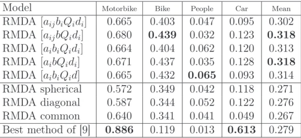
Model Motorbike Bike People Car Mean

RMDA [aijbiQidi] 0.665 0.403 0.047 0.095 0.302 RMDA [aijbQidi] 0.680 0.439 0.032 0.123 0.318 RMDA [aibiQidi] 0.664 0.404 0.062 0.120 0.313 RMDA [aibQidi] 0.671 0.437 0.035 0.128 0.318 RMDA [aibiQid] 0.665 0.432 0.065 0.093 0.314 RMDA spherical 0.572 0.349 0.042 0.118 0.271 RMDA diagonal 0.587 0.344 0.052 0.122 0.276 RMDA common 0.640 0.341 0.041 0.049 0.267 Best method of [9] 0.886 0.119 0.013 0.613 0.279

Table 2: Object localization results (AP measure) in the supervised case on the Pascal test 1 database for the 4 object categories (motorbikes, bicycles, people and cars).

Model Motorbike Bike People Car Mean

RMDA [aijbiQidi] 0.658 0.384 0.020 0.027 0.273 RMDA [aijbQidi] 0.686 0.404 0.038 0.020 0.287 RMDA [aibiQidi] 0.674 0.399 0.027 0.042 0.285 RMDA [aibQidi] 0.671 0.403 0.022 0.034 0.283 RMDA [aibiQid] 0.677 0.410 0.035 0.026 0.287 RMDA spherical 0.592 0.228 0.021 0.025 0.216 RMDA diagonal 0.603 0.234 0.044 0.027 0.227 RMDA common 0.655 0.293 0.015 0.021 0.246

Table 3: Object localization results (AP measure) in the weakly-supervised case on the Pascal test 1 database for the 4 object categories (motorbikes, bicycles, people and cars).

A.2. Object localization on Pascal test 2

Model Motorbike Bike People Car Mean

RMDA [aijbiQidi] 0.305 0.169 0.061 0.154 0.172 RMDA [aijbQidi] 0.316 0.164 0.091 0.151 0.181 RMDA [aibiQidi] 0.315 0.172 0.091 0.155 0.183 RMDA [aibQidi] 0.307 0.169 0.091 0.136 0.176 RMDA [aibiQid] 0.351 0.164 0.061 0.141 0.179 RMDA spherical 0.261 0.142 0.045 0.149 0.149 RMDA diagonal 0.245 0.153 0.091 0.156 0.161 RMDA common 0.301 0.163 0.045 0.147 0.164 Best method of [9] 0.341 0.113 0.021 0.304 0.112

Table 4: Object localization results (AP measure) in the supervised case on the Pascal test 2 database for the 4 object categories (motorbikes, bicycles, people and cars).

Model Motorbike Bike People Car Mean

RMDA [aijbiQidi] 0.304 0.141 0.021 0.115 0.145 RMDA [aijbQidi] 0.312 0.141 0.018 0.115 0.147 RMDA [aibiQidi] 0.311 0.161 0.045 0.049 0.142 RMDA [aibQidi] 0.298 0.153 0.026 0.116 0.148 RMDA [aibiQid] 0.322 0.141 0.023 0.034 0.130 RMDA spherical 0.254 0.111 0.023 0.037 0.106 RMDA diagonal 0.239 0.120 0.011 0.069 0.110 RMDA common 0.276 0.142 0.008 0.036 0.116

Table 5: Object localization results (AP measure) in the weakly-supervised case on the Pascal test 2 database for the 4 object categories (motorbikes, bicycles, people and cars).

References

[1] J. Banfield and A. Raftery. Model-based Gaussian and non-Gaussian clustering. Biometrics, 49:803–821, 1993.

[2] S. Bashir and E. Carter. High breakdown mixture discriminant analysis.

Journal of Multivariate Analysis, 93(1):102–111, 2005.

[3] R. Bellman. Dynamic programming. Princeton University Press, 1957. [4] H. Bensmail and G. Celeux. Regularized Gaussian discriminant analysis

through eigenvalue decomposition. Journal of the American Statistical

Association, 91:1743–1748, 1996.

[5] C. Bouveyron, S. Girard, and C. Schmid. High-Dimensional Data Clustering. Computational Statistics and Data Analysis, 52(1):502–519, 2007.

[6] C. Bouveyron, J. Kannala, C. Schmid, and S. Girard. Object localization by subspace clustering of local descriptors. In 5th Indian Conference on

Computer Vision, Graphics and Image Processing, pages 457–467, India,

2006.

[7] C. Brodley and M. Friedl. Identifying mislabeled training data. Journal

of Artificial Intelligence Research, 11:131–167, 1999.

[8] G. Celeux and G. Govaert. Parsimonious Gaussian models in cluster analysis. Pattern Recognition, 28:781–793, 1995.

[9] F. d’Alche Buc, I. Dagan, and J. Quinonero, editors. The 2005 Pascal

visual object classes challenge. Proceedings of the first PASCAL

Chal-lenges Workshop. Springer, 2006.

[10] B. Dasarathy. Noising around the neighbourhood: a new system struc-ture and classification rule for recognition in partially exposed environ-ments. IEEE Trans. Pattern Analysis and Machine Intelligence, 2:67–71, 1980.

[11] D. Gamberger, N. Lavrac, and C. Groselj. Experiments with noise filter-ing in a medical domain. In 16th International Conference on Machine

[12] G. Gates. The reduced nearest neighbor rule. IEEE Transactions on

Information Theory, 18(3):431–433, 1972.

[13] I. Guyon, N. Matic, and V. Vapnik. Discovering informative patterns and data cleaning. Advances in Knowledge Discovery and Data Mining, pages 181–203, 1996.

[14] T. Hastie and R. Tibshirani. Discriminant analysis by Gaussian mix-tures. Journal of the Royal Statistical Society B, 58:155–176, 1996. [15] T. Hastie, R. Tibshirani, and J. Friedman. The elements of statistical

learning. Springer, New York, 2001.

[16] D. Hawkins and G. McLachlan. High-breakdown linear discriminant analysis. Journal of the American Statistical Association, 92(437):136– 143, 1997.

[17] G. John. Robust decision trees: Removing outliers from databases. In

First conference on Knowledge Discovery and Data Mining, pages 174–

179, 1995.

[18] N. Lawrence and B. Schölkopf. Estimating a kernel Fisher discriminant in the presence of label noise. In Proc. of 18th International Conference

on Machine Learning, pages 306–313. Morgan Kaufmann, San Francisco,

CA, 2001.

[19] Y. Li, L. Wessels, D. de Ridder, and M. Reinders. Classification in the presence of class noise using a probabilistic kernel Fisher method.

Pattern Recognition, 40(12):3349–3357, 2007.

[20] D. Lowe. Distinctive image features from scale-invariant keypoints.

In-ternational Journal of Computer Vision, 60(2):91–110, 2004.

[21] G. McLachlan. Discriminant Analysis and Statistical Pattern

Recogni-tion. Wiley, New York, 1992.

[22] K. Mikolajczyk and C. Schmid. Scale and affine invariant interest point detectors. International Journal of Computer Vision, 60(1):63–86, 2004. [23] J. Mingers. An empirical comparison of pruning methods for decision

[24] J. Quinlan. Bagging, boosting and C4.5. In 13th National Conference

on Artificial Intelligence, pages 725–730, USA, 1996.

[25] P.J. Rousseeuw and A. Leroy. Robust Regression and Outlier Detection. Wiley, New York, 1987.

[26] Y. Sakakibara. Noise-tolerant occam algorithms and their applications to learning decision trees. Journal of Machine Learning, 11(1):37–62, 1993.

[27] R. Schapire. The strength of weak learnability. Machine Learning, 5:197– 227, 1990.

[28] G. Schwarz. Estimating the dimension of a model. The Annals of

Statis-tics, 6:461–464, 1978.

[29] P. Vannoorenbergue and T. Denoeux. Handling uncertain labels in multiclass problems using belief decision trees. In Proceedings of

IPMU’2002, 2002.

[30] D. Wilson and T. Martinez. Instance pruning techniques. In Fourteenth

International Conference on Machine Learning, pages 404–411, USA,

1997.

[31] X. Zeng and T. Martinez. A noise filtering method using neural net-works. In IEEE International Workshop on Soft Computing Techniques

in Instrumentation, Measurement and Related Applications, pages 26–

31, 2003.

[32] X. Zhu, X. Wu, and Q. Chen. Eliminating class noise in large datasets. In 20th ICML International Conference on Machine Learning, pages 920–927, USA, 2003.