Conservation Laws with Unilateral Constraints in Traffic Modeling

HAL Id: hal-00765427

https://hal.inria.fr/hal-00765427

Submitted on 14 Dec 2012

HAL is a multi-disciplinary open access

archive for the deposit and dissemination of sci-entific research documents, whether they are pub-lished or not. The documents may come from teaching and research institutions in France or

L’archive ouverte pluridisciplinaire HAL, est destinée au dépôt et à la diffusion de documents scientifiques de niveau recherche, publiés ou non, émanant des établissements d’enseignement et de recherche français ou étrangers, des laboratoires

Modeling

Rinaldo M. Colombo, Paola Goatin, Massimiliano D Rosini

To cite this version:

Rinaldo M. Colombo, Paola Goatin, Massimiliano D Rosini. Conservation Laws with Unilateral Constraints in Traffic Modeling. De Bernardis E. and Spigler R. and Valente V. Applied and Industrial Mathematics in Italy III, 82, Series on Advances in Mathematics for Applied Sciences, pp.244-255, 2009, �10.1685/CSC09XXX�. �hal-00765427�

ISSN 1827-9015, Vol. 3 (2009)

Conservation Laws with Unilateral Constraints

in Traffic Modeling

Rinaldo M. Colombo1, Paola Goatin2, Massimiliano D. Rosini3 1

Dipartimento di Matematica Via Branze 28, I-25123 Brescia, Italy

rinaldo@ing.unibs.it 2

I.S.I.T.V.

B.P. 56, 83162 La Valette du Var Cedex, France

goatin@univ-tln.fr 3

IM PAN

ul. Sniadeckich 8, 00956 Warszawa, Poland

mrosini@univaq.it

Keywords: Traffic Modeling, Conservation Laws, Nonclassical Shocks

Abstract

Macroscopic models for both vehicular and pedestrian traffic are based on conser-vation laws. The mathematical description of toll gates along roads or of the escape dynamics for crowds needs the introduction of unilateral constraints on the observable flow. This note presents a rigorous approach to these constraints, and numerical integra-tions of the resulting models are included to show their practical usability.

1. Introduction

The classical Lighthill–Whitham [22] and Richards [23] traffic model is based on the following simple assumptions:

1. The total number of vehicles is conserved.

2. The speed at a point is a function of the density at that point. Both assumptions appear perfectly suitable also for the macroscopic mod-eling of crowds. From the analytical point of view, in 1D, these assumptions lead to the conservation law

(1.1) ∂tρ + ∂xρ v(ρ) = 0

where the speed law v = v(ρ) plays a role analogous to that played by the equation of state for Euler equations of gas dynamics.

Along a highway, a toll gate acts as a unilateral constraint on the flow. Indeed, call q the given maximal flow of vehicles that can pass through the gate sited at, say, x = 0. Then, the resulting traffic can be reasonably described through (1.1) supplemented with

(1.2) ρ(t, 0) v ρ(t, 0)
≤ q .

(All BV functions, such as solutions to conservation laws, are assumed to be continuous from the left, so that their value is well defined at any point). Similarly, consider a crowd escaping along a corridor through an exit. Let q denote the maximal through flow at the exit sited, say, at x = 0. Then, again, equation (1.1) supplemented with (1.2) provides a simple though effective description of the escape dynamics. For other related descriptions of pedestrian dynamics, see [14,15,16,17,18,19].

Remark, however, that there is a key qualitative difference in the real evolutions of the two preceding examples. On one hand, the efficiency of the toll gate is not affected by the amount of vehicles lining up. On the other hand, as is well known, the crowd heading towards the exit may cause over-compression phenomena, possibly leading to panic, that may well reduce the efficiency of the exit. Therefore, in the case of pedestrians, we let the evolution of (1.1) be governed by nonclassical shocks.

The next section is devoted to the analytical results on (1.1)–(1.2). Section 3 deals with the toll gate model while Section 4 is devoted to the case of pedestrians.

2. Analytical Results

Following [8], we consider the Constrained Cauchy Problem (CCP)

(2.3)      ∂tρ + ∂xf (ρ) = 0 ρ(0, x) = ρo(x) f ρ(t, 0)
≤ q(t) under the standard assumptions

(CCP1) f ∈ C0_,1

[0, R]; R
, f(0) = f(R) = 0, there exists a ¯ρ ∈ ]0, R[ such that f′_{(ρ)(¯ρ − ρ) > 0 for a.e. ρ ∈ [0, R].}

(CCP2) q ∈ BV R+; [0, f (¯ρ)]
.

Note that in the case f (ρ) = ρ v(ρ), (2.3) reduces to the Cauchy Problem for (1.1)–(1.2).

To state the next well posedness result, it is useful to introduce the translation Ttthrough (Ttq)(τ ) = q(τ + t). Below we define a map S : R+×

D 7→ D, D being a suitable subset of L1

containing the initial data of (2.3). We then denote by ¯S the map ¯S : R+ × ¯D 7→ ¯D defined by ¯St(ρ, q) =

(Stρ, Ttq) with ¯D = D × BV.

Following [7,8,25], we use the nonlinear mapping Ψ(ρ) = sign(ρ − ¯ρ) f (¯ρ) − f (ρ)
.

Recall that by Riemann Problem we mean the following particular Cauchy Problem, see also [3, Chapter 5]:

(2.4)        ∂tρ + ∂xf (ρ) = 0 ρ(0, x) = ( ρl if x < 0 ρr if x > 0 .

Theorem 2.1. [8, Theorem 3.4] Let (CCP1) and (CCP2) hold. Then, for every constraint q ∈ BV R+; [0, f (¯ρ)]
there exists a map S : R+_{× D 7→ D}

such that

(S1) D ⊇nρ ∈ L1

R; [0, R]
: Ψ(ρ) ∈ BV(R; R)o;

(S2) ¯S is a Semigroup, i.e. ¯S0= Id and ¯St1◦ ¯St2 = ¯St1+t2;

(S3) S is non expansive in ρ, i.e. for all ρ1, ρ2 ∈ D

kStρ1− Stρ2kL1 ≤ kρ1− ρ2kL1;

(S4) if ρo and q are piecewise constant, then for t sufficiently small, Stρo

coincides with the gluing of the solutions to standard Riemann prob-lems centered at the points of jump of ρo and to (2.3) at x = 0;

(S5) for all ρo ∈ D, the orbit t 7→ Stρo yields a weak entropy solution

to (2.3), according to [8, definitions 3.1 and 3.2].

The proof uses the standard technique of wave front tracking, see [3, Chap-ters 6 and 7], and is deferred to [8]. The above statements (S1)–(S4) are clearly modeled on the definition of Standard Riemann Semigroup, see [3, Definition 9.1] and provide an analogue to it in the present constrained (and non autonomous) setting. The Lipschitz estimate (S3) is proved with suitable modifications of the classical techniques in [20] or [3, Section 6.3].

It is now easy to tackle the Initial Boundary Value Problem

(2.5)      ∂tρ + ∂xf (ρ) = 0 (t, x) ∈ R+× R− ρ(0, x) = ρo(x) x ∈ R− f ρ(t, 0)
≤ q(t) t ∈ R+.

Indeed, as in the case of the Riemann Problem, a solution to (2.5) is ob-tained restricting to x < 0 a solution to (2.3) with initial data, say, ρo(x) = 0

for x > 0. The extension to the general Initial Boundary Value Problem          ∂tρ + ∂xf (ρ) = 0 (t, x) ∈ R+× [0, L] ρ(0, x) = ρo(x) x ∈ [0, L] f ρ(t, 0)
= fo(t) t ∈ R+ f ρ(t, L)
≤ q(t) t ∈ R+

is immediate, see [9,13] and the references therein as a general reference on Initial Boundary Value Problems for scalar conservation laws.

In the case of pedestrians, the model presented in [10], see also [11,24], is based on a flow like that in Figure1. Note that this particular shape of the

Fig. 1. Left, a flow satisfying the requirements of Theorem2.2. Superimposed are the experimental measurements from [16]. Crowd density, ρ, is on the horizontal axis and flow, ρ v, on the vertical one. Right, another possible flow and the notation.

fundamental diagram was first postulated in [10] and then experimentally verified in [16]. Moreover, the evolution of the solutions to (1.1) is governed through the introduction of nonclassical shocks. That is, a Riemann Solver R is defined, which assigns to every pair ρl, ρrthe self similar weak solution

to the Riemann Problem (2.4) computed at time, say, t = 1.

As it is usual when dealing with nonclassical scalar conservation laws, see [21, Chapter II], we need first to introduce the auxiliary function ψ, see Figure 2, left. Let ψ(R) = R and, for ρ 6= R, let ψ(ρ) be such that the straight line through ρ, q(ρ)
and ψ(ρ), q ◦ ψ(ρ)
is tangent to the graph of q at ψ(ρ), q ◦ ψ(ρ)
. Besides, for ¯ρ ∈ [0, RT[ the line through ¯ρ, q(¯ρ)

and ψ(¯ρ), q ◦ ψ(ρ)
has a further intersection with the graph of q, which we call φ(¯ρ), q ◦ φ(¯ρ)
. Introduce two thresholds s and ∆s such that (2.6) s > 0 , ∆s > 0 , s < RM and R > s + ∆s ≥ φ(s) > RT > R − ∆s .

R R R∗ R∗ ρl ρr 0 s ∆s C N

Fig. 2. Left, the function ψ: its geometrical meaning. Right, the Riemann Solver: in C, the solution consists of classical waves only; in N , also nonclassical shocks are present.

We are now ready, following [11], to state the properties that allow to define R, see [10] for a slightly more general presentation, though limited to the Riemann Problem.

(R.1) If ρl_{, ρ}r_{∈ [0, R], then R(ρ}l_{, ρ}r_{) selects the classical solution unless}

ρl> s and ρr− ρl> ∆s .

In this case, R(ρl_{, ρ}r_{) consists of a nonclassical shock between ρ}l

and ψ(ρl_{), followed by the classical solution between ψ(ρ}l_{) and ρ}r_.

(R.2) If ρr_{< ρ}l_{, then R(ρ}l_{, ρ}r_{) is the classical solution.}

(R.3) If R ≤ ρl _{< ρ}r _{or ρ}l _{< R < ρ}r _{and the segment between (ρ}l_{, q(ρ}l₎₎

and (ρr_{, q(ρ}r_{)) does not intersect q = q(ρ), then the solution is a}

shock between ρl _{and ρ}r_.

(R.4) If ρl _{< R < ρ}r _{and the segment between (ρ}l_{, q(ρ}l_{)) and (ρ}r_{, q(ρ}r₎₎

intersects q = q(ρ), then R(ρl_{, ρ}r_{) consists of a nonclassical shock}

between ρl _{and a panic state followed by a possibly null classical}

wave. More precisely,

ρr_∈i_{R, ψ(ρ}l₎h_{: R(ρ}l_{, ρ}r_{) consists of a nonclassical shock between}

ρl _{and ψ(ρ}l_{), followed by a decreasing rarefaction between}

ψ(ρl_{) and ρ}r_;

ρr_∈h_ψ(ρl_{), R}∗h_{: R(ρ}l_{, ρ}r_{) consists of a single nonclassical shock.}

The Riemann Solver defined above is represented in Figure 2, right. Ac-cording to [10, Theorem 2.1], there exists a unique Riemann Solver defined by (R.1)–(R.4) which is consistent and L1

loc continuous in ˚C and ˚N , see

stability of the Cauchy Problem for (1.1). Refer to [10, I and II] or [8, Def-inition 2.2] for its precise statement.

In the next theorem, we refer to [11,24] for the precise statement of the conditions on the flow function. Here, it is sufficient to recall that both diagrams in Figure 1 do satisfy to all of them.

Theorem 2.2. [11, Theorem 3.4] Let f satisfy [10, (Q.1)–(Q.9)]. Let s, ∆s satisfy (2.6) and assume that there exists a constant W satisfying (2.7) W > 1 and φ(0) ψ(0) ≤ W + 1 2W ≤ ∆s ψ(s) − s. Then, for any initial datum ¯ρ ∈ (L1

∩BV) R; [0, R∗_{]
, the Cauchy Problem}

for (1.1) admits a nonclassical weak solution ρ = ρ(t, x) generated by the nonclassical Riemann Solver R and defined for all t ∈ R+. Moreover: (2.8) TV ρ(t)
≤ W · TV(¯ρ) , for all t ∈ R+.

3. Passing through a Toll Gate

This section is devoted to some numerical integrations of (2.3). Our aim is only to show that this model features reasonable qualitative proper-ties, hence we choose normalized parameters, leaving to future works the quantitative agreement with experimental data.

Let the real interval [0, 2] describe a segment of a highway with a toll gate at its center x = 1, as in Figure3 The evolution of traffic is described

000 000 000 000 000 111 111 111 111 111 0000000 1111111 00000001111111 0 1 x

Fig. 3. A toll gate sited at x = 1.

by (2.3) with, for instance, f (ρ) = ρ (1 − ρ). For simplicity, we assume that at time t = 0 vehicles are uniformly distributed between x = 0.2 and the site of the gate x = 1.

Assume that the initial density distribution is ρo(x) = 0.3 for x ∈ [0.2, 1]

and ρo(x) = 0 for x ∈ [0, 2] \ [0.2, 1]. The threshold of the through flow at

the gate is 0.1. Then, the computed time necessary for all the vehicles to pass the toll gate is t ≈ 2.4 and the evolution described by (2.3) is displayed in Figure4. As it has to be expected, the toll gate causes the rise of a queue to the left of the gate. This queue first increases an then decreases, finally disappearing when all vehicles passed the gate.

0.0 0.5 1.0 1.5 2.0 0.0 0.5 1.0 rho at time t=0 x rho 0.0 0.5 1.0 1.5 2.0 0.0 0.5 1.0 rho at time t=0.4 x rho 0.0 0.5 1.0 1.5 2.0 0.0 0.5 1.0 rho at time t=0.8 x rho 0.0 0.5 1.0 1.5 2.0 0.0 0.5 1.0 rho at time t=1.2 x rho 0.0 0.5 1.0 1.5 2.0 0.0 0.5 1.0 rho at time t=1.6 x rho 0.0 0.5 1.0 1.5 2.0 0.0 0.5 1.0 rho at time t=2 x rho

Fig. 4. Numerical integrations of (2.3) using Rusanov scheme, with f (ρ) = ρ (1 − ρ); ρo(x) = 0.3 for x ∈ [0.2, 1], ρo(x) = 0 for x ∈ R \ [0.2, 1] and q(t) = 0.1. The constraint at x = 1 is treated as suggested in [1].

We now let the initial density ρo of vehicles and the efficiency of the

gate q vary, while keeping the other parameters fixed. The time T that is necessary for all vehicles to pass the gate is then a function of ρoand q, that

is T = T (ρo, q). As it has to be expected, this function is monotone in both

variables, see Figure5. Note that as q → 0, obviously, T → +∞. Hence, in

0 5 10 15 20 T 0.0 0.2 0.4 0.6 0.8 1.0 ρ0 0.05 0.25 q 1.18 1.21 1.46 2 3 5 8 12 0.0 0.1 0.2 0.3 0.4 0.5 0.6 0.7 0.8 0.9 1.0 0.05 0.10 0.15 0.20 0.25 ρ0 q

Fig. 5. A density of ρo∈ [0.1, 1] vehicles is uniformly distributed on [0.2, 1]. A toll gate is sited at x = 1 and its through flow is q ∈ [0.05, 0.25]. T is the time necessary for all vehicles to pass the gate. Left, 3D diagram and, right, the level curves with ρo on the horizontal axis and q on the vertical one.

Figure5, T is computed only for q ≥ 0.04. Note the vertical segments in the level curves of T in Figure5, right. They realistically correspond to the gate being sufficiently efficient to avoid the rising of queues. On the contrary, as

soon as the toll gate influences the traffic flow, T is well approximated by a function of the ratio ρo/q, as also dimensional considerations suggest.

4. Pedestrian Evacuation and Braess Paradox

Consider now a corridor with space coordinate, say, x ∈ [0, L] with an exit at x = D, with 0 < D < L. Then, the dynamics of the crowd exiting the corridor is described by (2.3), with the standard Riemann Solver substituted by that prescribed through (R.1)–(R.4), see [11, Section 4.1] or [24, Section 2]. In emergency situations, it is well known that the pressure of the people seeking to exit may dramatically reduce the door efficiency. To prevent this, often suitable obstacles, typically columns, are posed in front of the exit, at a suitable distance, to partially sustain the crowd pressure.

In fact, the presence of an obstacle may avoid the insurgence of panic among the people, therefore keeping the door efficiency at a higher level. Paradoxically, the insertion of this obstacle may reduce the evacuation time, although most individuals may have a slightly longer path to reach the exit. This remarkable behavior reminds of the Braess paradox [2] typical of networks and is captured by the model presented in [10,11,24].

Assume now that an obstacle is placed in the corridor above at, say, x = d, with b < d < D. A group of people is uniformly distributed on the

0000000000 0000000000 0000000000 0000000000 1111111111 1111111111 1111111111 1111111111 0 a b d D x

Fig. 6. A corridor with an obstacle before the exit.

segment [a, b], with 0 < a < b < d, see Figure 6. Following Section 2 above and [11, Section 4], one is thus lead to integrate

(4.9)

(

∂tρ + ∂xf (ρ) = 0 f ρ(t, d−)
≤ q ρ(t, d−)

ρ(0, x) = ρo(x) f ρ(t, D−)
≤ Q ρ(t, D−)

with the evolution prescribed by the Riemann Solver defined by (R.1)– (R.4). The result is shown in Figure 7. As is well known, the efficiency of the exit may well be dramatically reduced when the crowd is panicking. Therefore, we assume that

(4.10) q(ρ) = ( ˆ q if ρ ∈ [0, R] ˇ q if ρ ∈ ]R, R∗_] with q > ˇˆ q, Q(ρ) =( ˆQ_ˇ if ρ ∈ [0, R] Q if ρ ∈ ]R, R∗_] with Q > ˇˆ Q.

0.0 0.9 1.8 2.7 3.6 0 3 6 9 12 rho at time t=0 x rho 0.0 0.9 1.8 2.7 3.6 0 3 6 9 12 rho at time t=1.8514286 x rho 0.0 0.9 1.8 2.7 3.6 0 3 6 9 12 rho at time t=3.0857143 x rho 0.0 0.9 1.8 2.7 3.6 0 3 6 9 12 rho at time t=3.7028571 x rho 0.0 0.9 1.8 2.7 3.6 0 3 6 9 12 rho at time t=5.5542857 x rho 0.0 0.9 1.8 2.7 3.6 0 3 6 9 12 rho at time t=8.0228571 x rho

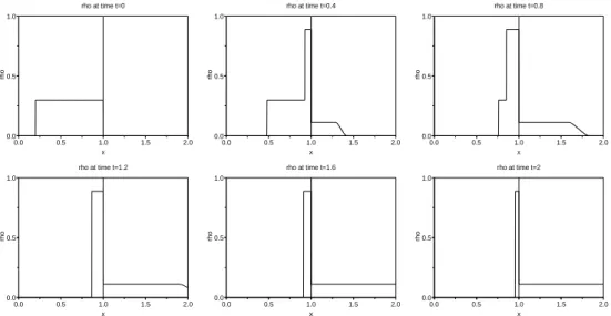
Fig. 7. Numerical integrations of (4.9) using the scheme in [4]. The vertical segments denote the positions of the obstacle and of the exit. The horizontal segments denote the maximal non-panic density R and the overall maximal density R∗_{. Here: a = 0.1, b = 1.1,} d= 2.45, D = 3.1 and L = 3.6. The constraints at x = d, D are treated as in [1].

The evacuation time T is particularly relevant and can be computed integrating (4.9)–(4.10) numerically following the procedure used in Sec-tion 3. Having a simple initial datum, i.e. uniformly distributed on a given segment, an analytical study is also possible. Indeed, the wave front track-ing technique applied to (4.9)–(4.10) yields Figure 8, right. In Figure 8, left, the same problem (4.9)–(4.10) is considered, but the obstacle is re-moved, i.e. q > max ρ v(ρ)
. Remarkably, in this particular situation, the evacuation time with no obstacle is larger than the evacuation time with the obstacle. The detailed construction of these solutions can be found in [11, Section 4.2]. Note that the darker regions in Figure8, left, represent where the crowd density attains panic values, i.e. ρ ∈ ]R, R∗_{]. The presence}

of the obstacle avoids the density to reach these high values, thus allowing for a faster evacuation from the room. In particular, we get the diagram in Figure9 for the evacuation time, T , as a function of the position of the ob-stacle, d ∈ ]b, D[. Note that when the obstacle is too near to the exit, i.e. to the right of the point K in Figure 8, left, its presence becomes negligible. Indeed, at K panic arises, while the efficiency of the obstacle is primarily dependent on avoiding it.

Fig. 8. Left, the structure of the solution to (4.9)–(4.10) with no obstacle, i.e. with q > max`ρ v(ρ)´; the evacuation time is tH. Right, the case with the obstacle, the evacuation time is tR.

Fig. 9. The dotted line is the evacuation time with no obstacle. The solid line is the evacuation time, T , as a function of the position of the obstacle, d. When the obstacle is too near to the exit, its presence becomes negligible.

5. Conclusions

We presented some analytical results on unilateral constraints in scalar conservation laws. They can be used to model real situations, such as

1. traffic flowing across a toll gate; 2. crowd evacuating a corridor.

In both cases, numerical integrations are possible, allowing a detailed de-scription of the phenomena. Furthermore, the times necessary for vehicles to cross the gate or for the people to exit the room can be computed.

Reasonable qualitative behaviors of the solutions are described. In par-ticular, in the case of pedestrians exiting a room, the model presented ac-counts for the possible decrease in the evacuation time thanks to the careful insertion of an obstacle at a well chosen position in front of the exit. This phenomenon, an analog of Braess paradox [2], is clearly non generic. Acknowledgments. The second author was partially supported by I.N.R.I.A. Sophia Antipolis - M´editerran´ee.

REFERENCES

1. Boris Andreianov, Paola Goatin and Nicolas Seguin. Finite volume schemes for locally constrained conservation laws. In preparation. 2. Dietrich Braess. ¨Uber ein Paradoxon aus der Verkehrsplanung.

Un-ternehmensforschung, 12:258–268, 1968.

3. Alberto Bressan, Hyperbolic systems of conservation laws. Oxford Uni-versity Press, 2000.

4. Christophe Chalons. Numerical approximation of a macroscopic model of pedestrian flows. SIAM J. Sci. Comput., 29(2):539–555 (electronic), 2007.

5. Christophe Chalons and Paola Goatin. Godunov scheme and sampling technique for computing phase transitions in traffic flow modeling. In-terfaces and Free Boundaries, 10(2):195–219, 2008.

6. Christophe Chalons and Paola Goatin. Transport-equilibrium schemes for computing contact discontinuities in traffic flow modeling. Commun. Math. Sci., 5(3):533–551, 2007.

7. Giuseppe M. Coclite and Nils H. Risebro. Conservation laws with time dependent discontinuous coefficients. SIAM J. Math. Anal., 36(4):1293– 1309 (electronic), 2005.

8. Rinaldo M. Colombo and Paola Goatin. A well posed conservation law with a variable unilateral constraint. J. Differential Equations, 234(2):654–675, 2007.

9. Rinaldo M. Colombo and Graziano Guerra On General Balance Laws with Boundary. Preprint, arXiv:0810.5246v1, 2008.

10. Rinaldo M. Colombo and Massimiliano D. Rosini. Pedestrian flows and non-classical shocks. Math. Methods Appl. Sci., 28(13):1553–1567, 2005.

11. Rinaldo M. Colombo and Massimiliano D. Rosini. Existence of non-classical solutions in a pedestrian flow model. Nonlinear Analysis: Real World Applications, to appear.

12. Constantine M. Dafermos, Hyperbolic conservation laws in continuum physics. Springer-Verlag, 2000.

13. Fran¸cois Dubois and Philippe Lefloch. Boundary conditions for nonlin-ear hyperbolic systems of conservation laws. J. Differential Equations, 71(1):93–122, 1988.

14. Dirk Helbing. A fluid-dynamic model for the movement of pedestrians. Complex Systems, 6(5):391–415, 1992.

15. Dirk Helbing, Ill`es Farkas and Tam`as Vicsek. Simulating dynamical features of escape panic. Nature, 407, September 28th 2000.

16. Dirk Helbing, Anders Johansson and Habib Zein Al-Abideen. Dynamics of crowd disasters: An empirical study. Physical Review E, 75(2), 2007. 17. Serge Hoogendoorn and Piet H. L. Bovy. Pedestrian route-choice and

activity scheduling theory and mode. Transp. Res. B, 2002.

18. Serge Hoogendoorn and Piet H. L. Bovy. Simulation of pedestrian flows by optimal control and differential games. Optimal Control Appl. Meth-ods, 24(3):153–172, 2003.

19. Roger L. Hughes. A continuum theory for the flow of pedestrians. Transportation Research Part B, 36:507–535, 2002.

20. Stanislav N. Kruˇzhkov. First order quasilinear equations with several independent variables. Mat. Sb. (N.S.), 81 (123):228–255, 1970. 21. Philippe G. Lefloch. Hyperbolic systems of conservation laws. Lectures

in Mathematics ETH Z¨urich. Birkh¨auser Verlag, Basel, 2002. The the-ory of classical and nonclassical shock waves.

22. Michael J. Lighthill and Gerald B. Whitham. On kinematic waves. II. A theory of traffic flow on long crowded roads. Proc. Roy. Soc. London. Ser. A., 229:317–345, 1955.

23. Paul I. Richards. Shock waves on the highway. Operations Res., 4:42– 51, 1956.

24. Massimiliano D. Rosini. Nonclassical interactions portrait in a pedes-trian flow model. J. Differential Equations, 246:408–427, 2009.

25. Blake Temple. Global solution of the Cauchy problem for a class of 2 × 2 nonstrictly hyperbolic conservation laws. Adv. in Appl. Math., 3(3):335–375, 1982.