Multiscale and multisolver pin power reconstruction approach in a reactor core calculation

HAL Id: cea-02509271

https://hal-cea.archives-ouvertes.fr/cea-02509271

Submitted on 16 Mar 2020

HAL is a multi-disciplinary open access

archive for the deposit and dissemination of

sci-entific research documents, whether they are

pub-lished or not. The documents may come from

teaching and research institutions in France or

abroad, or from public or private research centers.

L’archive ouverte pluridisciplinaire HAL, est

destinée au dépôt et à la diffusion de documents

scientifiques de niveau recherche, publiés ou non,

émanant des établissements d’enseignement et de

recherche français ou étrangers, des laboratoires

publics ou privés.

A. Targa, P. Le Tallec, J.-C. Le Pallec

To cite this version:

A. Targa, P. Le Tallec, J.-C. Le Pallec. Multiscale and multisolver pin power reconstruction approach

in a reactor core calculation. ICAPP 2015 - International Congress on Advances in Nuclear Power

Plants, May 2015, Nice, France. �cea-02509271�

Multiscale and multisolver pin power reconstruction approach in a reactor core

calculation

A.TARGA1,2, JC. LE PALLEC2, P. LE TALLEC1

1 _{Ecole Polytechnique, 91128 Palaiseau Cedex, France} 2 _{CEA/DEN/DANS/DM2S/SERMA, 91191 Gif sur Yvette Cedex, France}

targa@lms.polytechnique.fr

Abstract

-

I. INTRODUCTION

The Rod Ejection Accident (REA) is a fast power transient [1]. This accident leads to a fast and hard deformation of the power map (neutronics). Hence, it can induce gradual phenomena such as huge distortion or melting of the fuel elements (fuel pin thermal mechanics), boiling of the coolant (thermal hydraulics), clad failure and, potentially, fuel dispersion into the coolant [2]. This expresses the multidisciplinarity of the nuclear reactor system mainly in terms of neutronics, thermal mechanics and thermal hydraulics. A very important point concerning all these disciplines is the localization and scale effects of the phenomena, in terms of space and time dynamic [3]. Indeed, the fast and strong power incursion in the core leads to a heterogeneous and dissymmetrical spatial deposit of power on the fuel pin and the coolant, which might put the fuel pin into jeopardy. This transient occurs during a very short period of time and it can be decomposed in several laps according to the feedback reactions (e.g. Doppler effect and thermal dilatation) and the safety criterion that it might reach.

Consequently, a precise apprehension of the entire behavior of the reactor core requires at the very least the implementation of a multiphysics and multi-scale approach involving modeling of neutron behavior, fuel thermal mechanics [4] and thermal hydraulics [5].

Undoubtedly, on the one hand, a certain amount of studies and experimentations realized during the last 50 years give us a realistic description of the physical scenario. On the other hand, advances in computer science allow us to refine our modeling and calculation. This modeling evolution, from decoupling approach to “best estimate” calculations, is based on the simultaneous coupling of these discipline model equations and, more precisely, on the efficient management of the interactions between models, in terms of time dynamics and space/time accuracy, according to the physical scenario phenomenology.

The goal of this study is to respond to the need to access local parameters, i.e. power deposition inside the fuel pin and power deposition inside the coolant. This study should be the key to significantly improve the “Best Estimate” calculation effort started at the CEA and to balance the accuracy of modeling used in this coupling.

II. CONTEXT OF THE STUDY

This study is part of a work carried out in order to analyze PWR Nuclear reactor behavior in cases of standard and accidental (REA) situations through a multiphysics "Best Estimate" modeling. This work is using the SALOME [5] application named CORPUS, dedicated to best-estimate modeling of Pressurized Water Reactor (PWR) in normal and accidental

situations. One of the goals of this work is to get access to the local parameters at the fuel pin and sub channel scale. The other one is to properly and efficiently couple the different physics. This way, we concentrate our work only on the discipline of neutronics. The objective of this study is to access the local power deposit inside the fuel and the coolant (gamma fraction) using a two solver power reconstruction.

The pin power reconstruction method consists in computing simultaneously the unsteady 3D deterministic homogenized simplified transport equation solver over the whole core and the 3D deterministic heterogeneous transport solver over a single chosen assembly (typically the highest load assembly in terms of power). The homogeneous simplified transport solver is aimed to quickly produce coarse results for the transient scenario. On the other hand, the heterogeneous transport solver requires a very long calculation time but the results are more accurate. Hence, this method takes advantage of the calculation celerity of the homogeneous solver over the whole core, in order to compute a coarse flux that takes care of the environmental aspects of the flux distribution, as well

as of the accurate heterogeneous calculation solver over a single isolated assembly, in order to handle the precise flux distribution and to distinguish between the fuel pin and the fluid at the scale of the fuel pin, over this interesting subdomain of the core.

Several approaches and dynamics of the practical application of the modeling are possible. They are described in the following tab-1. The 3 steps of modeling developments of the tab-1 are defined according to their physical parameters, to boundary conditions, to the time evolution of the solver as well as to the type of the coupling used between solvers. At each step, an improvement of the modeling is brought to the coupling (colored words in bold letters highlight inputs of the new steps). Logically, our study focuses on the step 1 and will soon be followed by studies of the subsequent steps of modeling. This way, we are using the code APOLLO3® [6] which is a joined project of CEA, AREVA and EdF for the development of a new generation code system for the core physics analysis. Within APOLLO3® code we are working with the solver MINOS (SPn) and MINARET (Sn).

Modeling SPn Sn Coupling Scheme Local parameters Step 1 Mesh grid (scales)

Assemblies + assembly at the scale of the fuel cell Assembly at the scale of the fuel cell Cross sections

condensation

Assembly Fluid / Fuel pin

Domains (Boundary Conditions) Whole core (zero flux) Specific assembly (mirror)

Time evolution Kinetic calculation Static calculation

Step 2

Mesh grid Step 1 Step 1

Cross sections Assembly + Fuel cell step 1 Domains (Boundary Conditions) Whole core (zero flux) Specific assembly (SPn Flux)

Time evolution Kinetic calculation Static calculation

Step 3

Mesh grid Step1 Step 1

Cross sections Step 2 Step 1

Domains (Boundary Conditions) Whole core (zero flux) Specific assembly (SPn Flux)

Time evolution Kinetic calculation Kinetic calculation

Tab 1 – Tab of the dynamics of the practical application of the Pin Power reconstruction modeling.

P o st pro ce ss ing C o up lin g B o un da ry C o nd it io n C o up lin g B o un da ry C o nd it io n P o wer depo sit ins ide t he f uel (P comb) a nd po wer depo sit in side t he f lui d (P fluid ) Pcomb + P fluid Pcomb + Pfluid

III. MULTI-SCALE AND MULTI-SOLVER PIN POWER RECONSTRUCTION

Let us consider a domain Γ of ℝ3 and some subdomains γs  Γ, with s=1, 2,…, n. Over this entire

domain Γ, we are calculating the neutronic flux Φ_ΓG𝑖_(x)

with an energetic discretization according to the neutron macro energetic groups Gi. In addition, we are

calculating the flux Ψγ_s,∞

g_𝑖𝑗

(x,r), r  x, over extracted and isolated chosen subdomains γs, where gij are neutron

micro energetic group subdivisions of the macro energetic groups Gi and r a spatial discretization of the

variable x of this subdomain. For a specific subdomain γs, we are looking to rebuild the flux Φγs,core

g_𝑖𝑗

(x,r) which shall contain the information of the flux distribution from the whole domain Γ calculation but also the informations on the fine energetic and spatial discretization from the subdomain calculations. In other words, the calculation of the flux Φ_ΓG𝑖(x) gives us information about the whole distribution of the flux over the domain Γ (environment around the subdomain γs). The calculation of the flux Ψγs,∞

g_𝑖𝑗

(x,r), r  x, can be considered as a refinement calculation of specific subdomains in terms of energetic and spatial discretization.

In this configuration, the scalar flux Φ_ΓG𝑖_(x)

is calculated with an energetic discretization of Gi

macro groups and the scalar flux Ψ_γg_s,∞𝑖𝑗

(x,r) is calculated with an energetic discretization of gij micro groups that

can be considered as a refinement of the macro groups Gi , 𝑔𝑖𝑗 𝐺𝑖.

The neutron Transport equation

The two calculations are realized in parallel and separately from each other. On the first hand, the macro-groups flux Φ_ΓG𝑖_{(x) calculation is done with a}

zero flux boundary condition on the external surface δΓext of the domain Γ.

Φ_δΓG𝑖_{𝑒𝑥𝑡(x) = 0 (1)}

We assume that no neutrons are injected into the domain. This way, we resolve the transport and Kinetic equations detailed in [7]. 𝜕ΦΓ G_{𝑖(𝑥, Ω, 𝑡)} 𝜕𝑡 = 𝐷G𝑖 (𝑥, Ω, 𝑡) + 𝐷𝑖𝑠G𝑖 (𝑥, Ω, 𝑡) + 𝑆𝑐G𝑖 (𝑥, Ω, 𝑡) + 𝑆G𝑖 _{(𝑥, Ω, 𝑡) (2)}

The left term represents the time rate of neutron evolution in the system. The first term on the right represents the movement of neutrons into or out of the phase space volume of interest.

𝐷G_{𝑖 (𝑥, Ω, 𝑡) = − . (Ω Φ} Γ

G_𝑖

(𝑥, Ω, 𝑡))

The second term on the right accounts for all neutrons that disappear from that phase space by diffusion or absorption.

𝐷𝑖𝑠G_{𝑖 (𝑥, Ω, 𝑡) = − 𝛴} 𝑡

G_𝑖

(𝑥, 𝑡) Φ_ΓG𝑖_{(𝑥, Ω, 𝑡)}

The third term on the right accounts for all neutrons that collide in another phase space and appear into that phase space. 𝑆𝑐G𝑖 (𝑥_{, Ω, 𝑡) = ∑ (∫ dΩ}′_𝛴 𝑠 𝐺𝑖′ →G𝑖 _(𝑥 , Ω′_{→ Ω, 𝑡)Φ} Γ 𝐺𝑖′ _{(𝑥, Ω}′_{, 𝑡)} Я ) 𝐺 𝐺_𝑖′₌₁

The last term on the right 𝑆G𝑖 _{(x, Ω) is a source term}

from prompt and delayed fission source.

𝑆G_{𝑖 (𝑥, Ω, 𝑡) = 𝜒} 𝑝G𝑖(𝑥) ∑ 𝐵 𝜈 𝛴𝑡 G_𝑖 (𝑥, 𝑡)(𝐹(𝑥, 𝑡)) 𝐺 G_𝑖 =1 and (3) 𝐵 = (1 − 𝛽G_{𝑖 )} 𝐹(𝑥, 𝑡) = ∫ dΩΦ_ΓG𝑖 _{(𝑥, Ω, 𝑡)} Я + ∑(𝜆𝑖𝑐𝑖(𝑥, 𝑡) 𝜒𝑖 G_𝑖(𝑥)) 𝐿 𝑖=1 .

Here Φ_ΓG𝑖_{(𝑥, Ω, 𝑡) is the angular flux according to its}

energy interval Gi. The vector x represents the spatial

variable (x  R  R3). The unit vector Ω represents the traveling direction of a neutron. The direction Ω is expressed in terms of (θ,ϐ) in spherical coordinates, with θ the colatitude and ϐ the azimuthal angle. Я represents the unit sphere normalized to 1, ∫ _Я dΩ = 1. Σt, Σf and Σs are respectively the macroscopic isotropic

total, fission and anisotropic scattering cross-sections (C.S). 𝜒_𝑝G𝑖 designates the energy spectrum of prompt neutron of energy group Gi and 𝜒𝑖

G_𝑖

designates the energy spectrum of neutron precursor group i of energy group Gi. 𝛽𝑖

G_𝑖

is the delayed neutron fraction in energy group G𝑖 of precursor group i.

In addition, the density of precursor group cl is

governed by the Kinetic equation with l=1,..., L.

𝜕𝑐𝑙(𝑥,𝑡) 𝜕𝑡 = − 𝜆𝑙𝑐𝑙(𝑥, 𝑡) + Pr(𝑥, 𝑡) (4) with 𝑃𝑟(𝑥, 𝑡) = ∑ (𝛽_𝑙G𝑖 _𝜈G𝑖 𝛴 𝑓 G𝑖 _{(𝑥, 𝑡)(𝑃}𝛤_{(𝑥, 𝑡)))} 𝐺 G_𝑖 =1 𝑃𝛤_{(𝑥, 𝑡) = ∫ dΩ Φ} Γ G_{𝑖 (𝑥, Ω} , 𝑡) 4𝜋

which represent the fission products that may release energy by producing delayed neutrons. These 𝑐𝑙 nuclei

are called precursors. Hence, a precursor, identified by a family group of constants (𝜆𝑙 , 𝛽𝑙

G_𝑖

) that are the different life time 𝜆𝑙and their related delayed neutron proportion

𝛽_𝑙G𝑖_.

On the other hand, the flux Ψ_γg_s,∞𝑖𝑗 (x,r) calculation is done with a reflection boundary condition.

Ψ_δγg𝑖𝑗_{𝑒𝑥𝑡(r, Ω) = Ψ}

δγ𝑒𝑥𝑡

g_𝑖𝑗

(r, − Ω) (5)

We resolve the transport equation (2) in static condition [8] [9], which corresponds to solving an eigenvalue problem and leads to obtain a spectrum of eigenvalues and consequently of the flux. In this case the precursors are in equilibrium and the source term (3) takes the form:

𝑆g𝑖𝑗 (𝑟, Ω) = 1 𝑘𝑒𝑓𝑓𝜒𝑝 g𝑖𝑗_{(𝑟) ∑} (𝑆𝑓_{(𝑟, Ω)+𝑆}𝑒𝑥𝑡_{(𝑟, Ω))} 𝐺 g𝑖𝑗 =1 (6) with 𝑆𝑓_{(𝑟, Ω) = 𝜈 𝛴} 𝑓 g_𝑖𝑗 (𝑟) (∫ dΩ Ψ_γg_s,∞𝑖𝑗 _{(𝑟, Ω)} 4𝜋 )

where Ψ_γg_s,∞𝑖𝑗 _{(r,Ω,t) is the angular flux according to its}

energy interval gij, keff is the effective multiplication

factor, χ designates the fission spectrum, 𝜈 is the number of neutrons emitted per fission, Σ is the macroscopic fission cross-section.

Problem resolution

From the two flux expressed above (in their scalar form Φ_ΓG𝑖_{(x) and Ψ}

γ_s,∞

g_𝑖𝑗

(x,r)), at a time step ti of

the transient, we are aiming to obtain the flux

Φ_γg_s,core𝑖𝑗

(x,r), reconstructed by combining the most detailed space and energy representation of the pin cells spectra, i.e. the fine-group flux Ψ_γg_s,∞𝑖𝑗 (x,r), with the macrogroup flux Φ_ΓG𝑖 (x). The correction is done following the classical approach [10]:

Φ_γg_s,core𝑖𝑗 _{(x,r) = Φ} Γ G_{𝑖(x) . H} γs,∞ g_𝑖𝑗 (x,r) (7)

which introduces the fine-group shape factor by cell:

Hγs,∞

g𝑖𝑗 _{(x,r) =} Ψγs,∞g𝑖𝑗 (x,r)

∑_𝑔𝑖𝑗  𝐺𝑖(∫_𝑟x (Ψ_γs,∞g𝑖𝑗 (x,r)𝑑𝑟)) .

Ψ_γs,∞g𝑖𝑗 (x)

<Ψ_γs,∞g𝑖𝑗 (x)>_γs,∞ . (8)

Observe that we have by construction, ∑ (∫ Hγ_s,∞

g_𝑖𝑗

(x, r)𝑑𝑟

𝑟γs

𝑔_𝑖𝑗  𝐺𝑖 ) = 1. (9)

Therefor the reconstructed flux preserves the correct value of the integral of the flux over the subdomain x

 γ𝑠: ∑ (∫ Φγs,core g_𝑖𝑗 (x, r)𝑑𝑟 𝑟γs 𝑔_𝑖𝑗  𝐺_𝑖 ) = ΦΓ G_𝑖 (x) (10)

The flux over the whole core does not distinguish between the fuel cells that contain fuel pellet and the others that contain guide tube (without any fuel). It considers the assembly as a homogeneous block refined at the scale of the fuel cell. Meanwhile, the single heterogeneous assembly calculation does make this distinction and produces a very precise flux distribution in terms of space and mediums that compose the assembly.

Power computation

Traditionally, the computation of the power inside the fluid consists in multiplying the Power of the homogeneous fuel cell by a constant experimental factor [11]. Meanwhile, this pin power reconstruction method allows us to distinguish between the Power inside the fuel pin and inside the fluid. The power production is defined as below:

𝑃𝑣𝑜𝑙 𝑚 (x) = ∑ ∫ (χ𝑔𝑖𝑗 Σ𝑔𝑖𝑗(x, r)Ψ𝑔𝑖𝑗(x, r))

𝑟x

𝐺

𝑔𝑖𝑗=1

dr (14)

Where the symbol m represents the fuel (f) or the fluid moderator (mod) medium in r of the fuel cell x, r  x.

Pin Power Reconstruction methodology

At each step of the transient calculation, the mentioned above method is used to rebuild the Pin Power. The algorithm to compute the transient scenario is established through several phases detailed below:

• Phase 0 - First time step: Simultaneous initialization

of both calculations. Both solvers are set respecting the same initial conditions (Burn up map, temperatures, density, isotopic concentration, etc.);

• Phase 1 – MINOS neutronic transient calculation at

time step ti and MINARET neutronic static calculation

for the current parameters.

• Phase 2 - Post-treatment of the MINOS flux: it

consists in multiplying it by a shape factor that is derived from the fine MINARET flux;

• Phase 3 - Calculation of the power inside the fuel and

the fluid, with the normalization of the post-treated flux by the MINOS total power, over the assembly of interest. This operation leads to the conservation of the total power and consequently of the reaction rate inside the studied assembly;

• Phase 4 – Modification of thermo-mechanic and

thermo-hydraulic parameters in MINOS;

• Phase 5 - Updating of the Cross Sections according to

the control rod ejection evolution, thermo-mechanic and thermo-hydraulic parameters;

• Phase 6 - New time step: return to phase 1.

IV. ROD EJECTION ACCIDENT SCENARIO

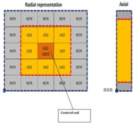
In order to simplify the implementation of the coupling scheme we are initially working on a small core reactor. This reactor is a 5x5 geometry reactor made of 9 internal fuel assemblies and an external ring of 16 reflectors (figure 1).

It has a power of 177.2MW, and is 468.72 cm in height. The central assembly contains the control rod. Hence, the neutronic static calculation would be done over an isolated assembly corresponding to the lateral assembly nearby the central one. According to studies on REA [13], this assembly corresponds to the highest load assembly in terms of power. Indeed, the hot spot does not appear in the assembly where the control rod had been ejected but within its nearest lateral neighbor

[13]. Nevertheless, the static calculation could easily be realized on every other assembly of the core. Thanks to this reactor core modeling, the coupling scheme analysis and the simulation shall be significantly simplified in terms of computation time and data analysis. However, this geometry preserves the physical, neutronic and mechanical specificities as well as the behaviors of the PWR 1300MWe in case of nominal and accidental situations. Specular conditions are imposed as boundary conditions of the two domains, i.e. MINOS uses a void boundary condition and MINARET uses a mirror boundary condition.

Figure 1 - Reactor 5x5 geometry scheme

We assume that before the transient the power inside the core is constant and the neutron population balance is stable. When the rod is ejected the balance is broken. In this study we focus on hot zero power which would lead the reactor to go prompt critical, producing a rapid power spike of about several milliseconds, increasing from quasi-zero to about ten times the nominal power. In addition, the core is set at the start of the fuel cycle process (Burn-up = 0 MWj/d) for all its assemblies. The control rod system is only contained by the central assembly. For these reasons we arbitrarily draw the neutronic parameter of the rod as well as of the whole core from the previous study [3] [12] [13]. The refinement of the grid is done in this specific assembly at the scale of the fuel cell and at the scale of the fuel pin for the single Sn assembly.

The Rod ejection accident (REA) is based on assuming that there is a mechanical failure of the housing of a control rod drive mechanism so that the internal pressure in the core (Pint = 155 bar) forces the mechanism out (Pext = 1 bar) and the attached control rod assembly is ejected vertically from the reactor. This difference in pressure pulls the control rod out with an acceleration of about 22 g and thus in about 0.1s [1]. During the ejection period, only the neutronic discipline

is affected. We decide to limit our study to this brief moment. This choice gives us the right to focus on the neutronic Pin Power Reconstruction without any feedback effect. In conclusion, we neglect the thermal, mechanical and hydraulic aspects of the rest of the scenario, which are going to be used and analyzed during the next coupling study. This way, the macroscopic cross section 𝛴_{𝑛𝑢𝑐𝑙𝑒𝑎𝑟 𝑟𝑒𝑎𝑐𝑡𝑖𝑜𝑛}𝐸𝑛𝑒𝑟𝑔𝑦 𝑔𝑟𝑜𝑢𝑝 would only evolve according to the control rod axial changes inside the core.

V. RESULTS

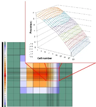
First, we can observe one of the power maps from the phase 1 MINOS Kinetic calculation, at a representative time step ti, as it is expressed in “Pin Power

Reconstruction methodology” of the previous section.

For purposes of the present paper, the power reconstruction was only performed in 2D.

The shape of the power map is applied over the solver grid (hybrid due to the junction between the single nodes of the refined assembly and the external surface boundary). In the best case of the assembly we are interested in, the power we obtain is homogenized to the fuel cell (figure 2) where we do not distinguish the fuel pin from the fluid, according to the mesh grid accuracy of the SPn solver and C.S.

Figure 2 – MINOS SPn homogeneous core power maps calculation

Next, we obtain an accurate distribution of the power inside the single assembly calculated with the Sn

solver (figure 3). This way, we properly distinguish the guide tube from the fuel pin. Unfortunately, this single assembly power distribution (symmetrical) does not take into account the environmental aspects of the flux distribution that is dealt with in the whole core calculation.

Figure 3 – MINARET Sn Single Assembly pin power maps calculation

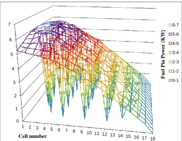
Moreover, the Sn solver calculation provides us with a very accurate flux distribution that allows us to calculate the ratio between the power deposition inside the fluid and the fuel pin (figure 4).

Figure 4 – MINARET Sn Single Assembly Accurate Power distribution

Hence, in a second time, through the Pin Power Reconstruction methodology that we have defined in the previous section, we obtained two distinct and

accurate power maps over the assembly of interest. In the first one (figure 5), we observe the precise post processed map of the power deposit inside the fuel.

Figure 5 – Post processed map of power deposit inside the fuel pin

In the second one (figure 6), we observe the post processed map of the power deposit inside the fluid. This was not accessible in the original MINOS calculation. The fluid is composed mainly of water (H2O) and also of a tiny but significant portion of Boron. The Hydrogen as well as the Boron has a moderating effect on the neutron celerity. Indeed, the scattering cross sections of both nuclei are huge and induce a significant amount of inelastic collision with the neutron. We effectively find this physical effect in addition to the gamma fraction in the map of the power deposit inside the fluid due to the cross sections production that takes into account these phenomena. These distributions of the fluid and fuel pin power fraction shall take all their significance during the multiphysics coupling.

Figure 6 – Post processed map of power deposit inside the fluid

These figures merely serve to illustrate the results we got from our study, where we performed a Best Estimate neutronics calculation at a representative time step ti. Indeed, during an equivalent computing

time we obtained environmental informations over the whole core, by the SPn MINOS calculation, and a very precise distribution of the power separately inside the fuel pins and the fluid by the Sn MINARET calculation over a single assembly.

This power post treatment reconstruction can be applied to the phase 1 of each time step ti of the

transient calculation illustrated below, in the (figure 7). This figure represents a REA scenario computed using the MINOS Kinetic solver calculation.

Figure 7 – Power and Energy evolution during REA transient scenario [12]

VI. CONCLUSION

The Pin power reconstruction method that we develop in the paper allows us to precisely distinguish the contribution of the power deposit inside the fuel pin and inside the fluid. This computation is obtained by a post proceeding of a whole core deterministic homogeneous calculation (which takes care of the environmental aspects of the flux distribution) by a single assembly deterministic heterogeneous calculation (that handles the precise flux distribution at the scale of the fuel pin).

This choice of the Pin Power Reconstruction post treatment approach has simplified the implementation and provides flexibility in achieving a variety of reconstructions in terms of localization of the

0 1 2 3 4 5 6 7 1 2 3 4 5 6 7 8 9 10 11 12 13 _{14 15 16 17 18} F u el P in P o w er ( KW ) Cell number 6-7 5-6 4-5 3-4 2-3 1-2 0-1 0 0,005 0,01 0,015 0,02 0,025 0,03 0,035 1 ₃ 5 7 ₉ 11 ₁₃ 15 ₁₇ F lu id P owe r (k W) Cell number 0,03-0,035 0,025-0,03 0,02-0,025 0,015-0,02 0,01-0,015 0,005-0,01 0-0,005

assembly of interest and in terms of geometry. This method should be easily adapted to a case of a PWR 1300MWe or inserted into a multiphysics-multiscale modeling. Moreover, the discretization inside the fuel pin or inside the fluid should be improved in order to take care of the Rim effects.

In addition, this process will soon be followed by similar processes of study of the subsequent steps of modeling that we discussed in tab 1. Finally, a stochastic calculation could be done and compared with the calculation all together in order to definitively validate our approach and to determine the best method to be used in the framework of a multiphysics-multiscale Best Estimate coupling.

VII. ACKNOWLEDGEMENTS

The authors are very grateful to CEA and Ecole Polytechnique collaborators for their valuable support during this work, especially Mrs. BAUDRON, Mr. LAUTARD and Mr. SCHNEIDER.

REFERENCES

1. B. TARRIDE, ’Physique, fonctionnement et sureté des

REP: Maitrise des situations accidentelles du système réacteur, Collection Génie Atomique, EDP science, 318

pages, 2013.

2. M. LE SAUX, Comportement et rupture de gaines en

Zircaloy-4 détendu vierge hydrurée ou irradiées en situation accidentelle de type RIA, Rapport CEA-R-6248

CEA-Ecole des Mines de Paris, 2008.

3. J.C. LE PALLEC, Analyse d’un accident de réactivité

induit par l’éjection d’une grappe sur un cœur REP1300 MWe chargé en combustible CORAIL, Rapport CEA,

SERMA/LCA/RT/03-3349, 2004.

4. K. MER-NKONGA, N. CROUZET, J-C. LE PALLEC, B. MICHEL, D. SCHNEIDER and A. TARGA, ’’Coupling of fuel performance and neutronic codes for PWR’’, 11th World Congress on Computational

Mechanics (WCCM XI), 5th European Conference on Computational Mechanics (ECCM V), 6th European Conference on Computational Fluid Dynamics (ECFD VI), Barcelona, Spain, July 20-25, 2014.

5. D. SCHNEIDER, J.C. LE PALLEC, A. TARGA, ’’Mise en œuvre d’un exercice de couplage APOLLO3-FLICA4 dans l’outil Multi Physique CORPUS dédié à l’analyse des réacteurs REP en situations de fonctionnement normal et accidentel’’, Journée Utilisateurs SALOME, CEA-Saclay, 21 novembre 2013.

6. H. GOLFIER, R. LENAIN, C. CALVIN, J-J. LAUTARD, A-M. BAUDRON, Ph. FOUGERAS, Ph. MAGAT, E. MARTINOLLI, Y. DURTHEILLET, ’’APOLLO3: a common project of CEA, AREVA and EDF for the development of a new deterministic multi-purpose code for core physics analysis’’, International

Conference on Mathematics, Computational Methods and Reactor Physics, Saratoga Springs, New York, May

3-7, 2009.

7. A.M. BAUDRON, J.J. LAUTARD, ’’MINOS: A Simplified Pn Solver for Core Calculation’’, Nuclear

Science and Engineering, 155(2), pp.250-263, February

2007.

8. J.Y. MOLLER and J.J. LAUTARD, ’’MINARET, a deterministic neutron transport solver for nuclear core calculations’’, International Conference on Mathematics

and Computational Methods Applied to Nuclear Science and Engineering (M&C 2011) Rio de Janeiro, RJ, Brazil,

Latin American Section (LAS) / American Nuclear Society (ANS), May 8-12, 2011.

9. O. MULA HERNÁNDEZ, ’’Quelques contributions vers

la simulation parallèle de la cinétique neutronique et la prise en compte de données observées en temps réel’’,

Mémoire de thèse, Université Pierre et Marie Curie, tel-01068691, septembre 2014.

10. I. ZMIJAREVICc, E. MASIELLO and R. SANCHEZ, ’’Flux reconstruction methods for assembly calculations in the code APOLLO2’’, PHYSOR-2006, ANS Topical Meeting on Reactor Physics Organized and hosted by the Canadian Nuclear Society, Vancouver, BC, Canada. 2006 September 10-14.

11. P. Raymond, ’’FLICA3 v3.2. Equations Models’’. Technical report DMT/92- 139, CEA 1992.

12. R. CAPANNA, ’’Contribution to the development of a calculation scheme into the code APOLLO3® dedicated to the modeling of an accident scenario of type RIA in a nuclear power plant’’, Master Thesis, Politecnico Milano

, December 2014.

13. J.C. LE PALLEC, ’’Modélisation réaliste d'un accident

de réactivité dans les REP et analyse d'incertitudes,

Mémoire de thèse, Institut National Polytechnique de Grenoble, 2002.