HAL Id: inria-00606739
https://hal.inria.fr/inria-00606739
Submitted on 22 Jul 2011
HAL is a multi-disciplinary open access
archive for the deposit and dissemination of
sci-entific research documents, whether they are
pub-lished or not. The documents may come from
teaching and research institutions in France or
abroad, or from public or private research centers.
L’archive ouverte pluridisciplinaire HAL, est
destinée au dépôt et à la diffusion de documents
scientifiques de niveau recherche, publiés ou non,
émanant des établissements d’enseignement et de
recherche français ou étrangers, des laboratoires
publics ou privés.
Breaking the 64 spatialized sources barrier
Nicolas Tsingos, Emmanuel Gallo, George Drettakis
To cite this version:
Nicolas Tsingos, Emmanuel Gallo, George Drettakis. Breaking the 64 spatialized sources barrier.
[Research Report] Inria. 2003, pp.8. �inria-00606739�
Breaking the 64 spatialized sources barrier
Nicolas Tsingos, Emmanuel Gallo and George Drettakis
REVES / INRIA-Sophia Antipolis
http://www-sop.inria.fr/reves
Spatialized soundtracks and sound-effects are standard elements of today’s video games. However, although 3D audio modeling and content creation tools (e.g., Creative Lab’s EAGLE [4]) provide some help to game audio designers, the number of available 3D audio hardware channels remains limited, usually ranging from 16 to 64 in the best case. While one can wonder whether more hardware channels are actually required, it is clear that large numbers of spatialized sources might be needed to render a realistic environment. This problem becomes even more significant if extended sound sources are to be simulated: think of a train for instance, which is far too long to represented as a point source. Since current hardware and APIs implement only point-source models or limited extended source models [2,3,5], a large number of such sources would be required to achieve a realistic effect (view Example1). Finally, 3D-audio channels might also be used for restitution-independent representation of surround music tracks, leaving the generation of the final mix to the audio rendering API but requiring the programmer to assign some of the precious 3D channels to the soundtrack. Also, dynamic allocation schemes currently available in game APIs (e.g. Direct Sound 3D [2]) remain very basic. As a result, game audio designers and developers have to spend a lot of effort to best-map the potentially large number of sources to the limited number of channels. In this paper, we provide some answers to this problem by reviewing and introducing several automatic techniques to achieve efficient hardware mapping of complex dynamic audio scenes in the context of currently available hardware resources.
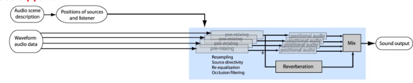
Figure 1 - A traditional hardware-accelerated audio rendering pipeline. 3D audio channels process the audio data to reproduce distance, directivity, occlusion, Doppler shift and positional audio effects depending on the 3D location of the source and listener. Additionally, a mix of all signals is generated to feed an artificial reverberation or effect engine.
We show that clustering strategies, some of them relying on perceptual information, can be used to map a larger number of sources to a limited number of channels with little impact to the perceived audio quality. The required pre-mixing operations can be implemented very efficiently on the CPU and/or the GPU (graphics processing unit), out-performing current 3D audio boards with little overhead. These algorithms simplify the task of the audio designer and audio programmer by removing the limitation on the number of spatialized sources. They permit rendering of extended sources or discrete sound reflections, beyond current hardware capabilities. Finally, they integrate well with existing APIs and can be used to drive automatic resource allocation and level-of-detail schemes for audio rendering.
In the first section, we present an overview of clustering strategies to group several sources for processing through a single hardware channel. We will call such clusters of sources auditory impostors. In the second section, we describe recent techniques developed in our research group that incorporate perceptual criteria in hardware channel allocation and clustering strategies. The third section is devoted to the actual audio rendering of auditory impostors. In particular, we present techniques maximizing the use of all available resources including the CPU, APU (audio processing unit) and even the GPU which we turn into an efficient audio processor for a number of operations. Finally, we demonstrate the described concepts on several examples featuring a large number of dynamic sound sources1.
1 The soundtrack of the example movies was generated using binaural processing. Please, use headphones for
Figure 2- Clustering techniques group sound sources (blue dots) into groups and use a single representative per cluster (colored dots) to render or spatialize the aggregate audio stream.
Clustering sound sources
The process of clustering sound sources is very similar in spirit to the level-of-detail (LOD) or impostor concept introduced in computer graphics [13]. Such approaches render complex geometries using a smaller number of textured primitives and can scale or degrade to fit specific hardware or processing power constraints whilst limiting visible artefacts. Similarly, sound-source clustering techniques (Figure 2) aim at replacing large sets of point-sources with a limited number of representative point-sources, possibly with more complex characteristics (e.g. impulse response). Such impostor sound-sources can then be mapped to audio hardware to benefit from dedicated (and otherwise costly) positional audio or reverberation effects (see Figure 3). Clustering schemes can be divided into two main categories: fixed clustering, which uses a predefined set of clusters, and adaptive clustering which attempts to construct the best clusters on-the-fly. Two main problems in a clustering approach are the choice of a good clustering criteria and a good cluster representative. The answers to these questions largely depend on the available audio spatialization and rendering back-end and whether the necessary software operations can
be performed efficiently. Ideally, the clustering and rendering pipeline should work together to produce the best result at the ears of the listener. Indeed, audio clustering is linked to human perception of multiple simultaneous sound sources, a complex problem that has received a lot of attention in the acoustics community [7] . This problem is also actively studied in the community of auditory scene analysis (ASA) [8,16]. However, ASA attempts to solve the dual and more complex problem of segregating a complex sound mixture into discrete, perceptually relevant components.
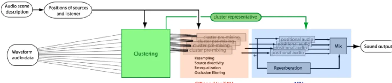
Figure 3 - An audio rendering pipeline with clustering. Sound sources are grouped into clusters which are processed by the APU as standard 3D audio buffers. Constructing the aggregate audio signal for each cluster must currently be done outside the APU, either using the CPU and/or GPU.
Fixed-grid clustering
The first instance of source clustering was introduced by Herder [21,22] in 1991 who grouped sound sources by cones in direction space around the listener, the size of which was chosen relying upon available psycho-acoustic data on the spatial resolution of human 3D hearing. He also discussed the possibility of grouping the sources by distance or relative-speed to the listener. However, it is unclear that relative speed, which might vary a lot from source to source is a good clustering criteria. One drawback of fixed grid clustering approaches is that they cannot be targeted to fit a specified number of (non-empty) clusters. Hence, they can end-up being sub-optimal (e.g., all sources fall into the same cluster while sufficient resources are available to process all of them independently) or might provide too many non-empty clusters for the system to render any further (see Figure 5). It is however possible to design a fixed grid clustering approach that works pretty well by using direction-space clustering and more specifically “virtual surround”. Virtual surround renders the audio from a virtual rig of loudspeakers (see Figure 4). Each loudspeaker can be mapped to a dedicated hardware audio buffer and spatialized according to its 3D location. This technique is widely used for headphone rendering of 5.1 surround
Figure 4 - “Virtual surround”. A virtual set of speakers (here located at the vertices of an icosahedron surrounding the listener) are used to spatialize any number of sources using 18 3D audio channels.
film soundtracks (e.g., in software DVD players), simulating a planar array of speakers. Extended to 3D, it shares some similarities with directional sound-field decomposition techniques such as Ambisonics [34]. However, not relying on complex mathematical foundations, it is less accurate but does not require any specific audio encoding/decoding and fits well with existing consumer audio hardware. Common techniques (e.g. amplitude panning [31]) can be used to compute the gains that must be applied to the audio signals feeding the virtual loudspeakers in order to get smooth transitions between neighboring directions. The main advantage for such an approach is its simplicity. It can be very easily implemented in an API such as DirectSound 3D (DS3D). The main application is responsible for the pre-mixing of signals and panning calculations while the actual 3D sound restitution is left to DS3D. Although there is no way to enforce perfect synchronization between DS3D buffers, the method appears to work very well in practice. Example 2 and Example 3 feature a binaural rendering of up to 180 sources using two
different virtual speaker rigs (respectively an octahedron and an icosahedron around the listener) mapped to 6 and 18 DS3D channels. One drawback of a direction-space approach is that reverberation-based cues for distance rendering, e.g., in EAX [3] which implements automatic reverberation tuning based on source-to-listener distance, can no longer be used directly. One work-around this issue is to use several virtual speaker rigs located at different distances from the listener, at the expense of more 3D channels.
Adaptive positional clustering
In contrast to fixed-grid methods, adaptive clustering aims at grouping sound sources based on their current 3D location (including incoming direction and distance to the listener) in an “optimal” way. Adaptive clustering has several advantages: 1) it can produce a requested number of non-empty clusters, 2) it will automatically refine the subdivision where needed, 3) it can be controlled by a variety of error metrics. Several clustering approaches exist and can be used for this purpose [18,19,24]. For instance, global k-means techniques [24] start with a single cluster and progressively subdivide it until a specified error criteria or number of clusters has been met. This approach constructs a subdivision of space that is locally optimal according to the chosen error metric. Example 4 shows the result of such an approach applied to a simple example where three spatially-extended sources are modeled as a set of 84 point-sources. Note the progressive de-refinement when the number of clusters is reduced and the adaptive refinement when the listener is moving closer or away from the large “line-source”. In this case, the error metric was a combination of distance and incident direction onto the listener. Cluster representatives were constructed as the centroid in polar coordinates of all sources in the cluster.
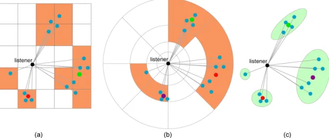
Figure 5 – Fixed grid and adaptive clustering illustration in 2D. (a) regular grid clustering (ten non-empty clusters), (b) non-uniform “azimuth-log(1/distance)” grid (six non-empty clusters), (c) adaptive clustering. Contrary to fixed grid clustering, adaptive clustering can « optimally » fit a predefined cluster budget (four in this case).
Perceptually-driven source prioritization and resource allocation
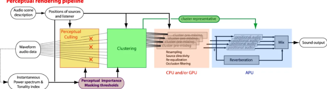
So far, very few approaches have attempted to include psycho-acoustic knowledge in the audio rendering pipeline. Most of the effort has been dedicated to speeding up signal processing cost for spatialization purposes, e.g. spatial sampling of HRTF or filtering operations for headphone rendering [6,28]. However, existing approaches never consider the characteristics of the input signal. On the other hand, important advances in audio compression, such as MPEG-1 layer 3 (mp3), have shown that exploiting both input signal characteristics and our perception of sound could provide unprecedented quality vs. compression ratios [15,25,26]. Thus, taking into consideration signal characteristics in audio rendering might help to design better prioritization and resource allocation schemes, perform dynamic sound source culling and improve the construction of clusters. However, contrary to most perceptual audio coding (PAC) applications, that encode once to be played repeatedly, the soundscape in a video game is highly dynamic and perceptual criteria have to be recomputed at each processing frame for a possibly large number of sources. We propose a perceptually-driven audio rendering pipeline with clustering, illustrated in Figure 6.Figure 6 – A perceptually-driven audio rendering pipeline with clustering. Based on pre-computed information on the input signals, the system dynamically evaluates masking thresholds and perceptual importance criteria for each sound source. Inaudible or masked sources are discarded. Remaining sources are clustered. Perceptual importance is used to select better cluster representatives.
Prioritizing sound sources
Assigning priorities to sound sources is a fundamental aspect of resource allocation schemes. Currently, APIs such as DS3D use basic schemes based on distance to the listener for on-the-fly allocation of hardware channels. Obviously, such schemes would benefit from the ability to sort sources by perceptual importance or “emergence” criteria. As we already mentioned, this is a complex problem, related to the segregation of complex sound mixtures as studied in the ASA field. We experimented with a simple, loudness-based model that appears to give good results in practice, at least in our test examples. Our model uses power spectrum density information pre-computed on the input waveforms (for instance, using short time Fast Fourier Transform) for several frequency bands. This information does not represent a significant overhead in terms of memory or storage space. In real-time, we access this information, modify it to account for distance attenuation, directivity of the source, etc., and map the value to perceptual loudness space using available loudness contour data [11,32].
We use this loudness value as a priority criterion for further processing of sound sources.
Dynamic sound source culling
Sound source culling aims at reducing the set of sound sources to process by identifying and discarding inaudible sources. A basic culling scheme determines whether the source amplitude is below the absolute threshold of hearing (or below a 1-bit amplitude threshold). Using dynamic loudness evaluation for each source, as described in the previous section, makes this process much more accurate and effective. Perceptual culling is a further refinement aiming at discarding sources that are perceptually masked by others. Such techniques have been recently used to speed-up modal/additive synthesis [29,30], e.g., for contact-sound simulation. To exploit them for sampled sound signals, we pre-compute another characteristics of the input waveform, the tonality. Based on PAC techniques, an estimate of the tonality in several sub-bands can be calculated using short-time FFT. This tonality index [26] estimates whether the signal in each sub-band is closer to a noise or a tone. Masking thresholds, which typically depend on such information, can then be dynamically evaluated. Our perceptual culling algorithm sorts the sources by perceptual importance, based on their loudness and tonality, and progressively inserts them into the current mix. The process stops when the sum of remaining sources is masked by the sum of already inserted sources. In a clustering pipeline, sound source culling could be used either before or after clusters are formed. Both solutions have their own advantages and drawbacks. Performing culling first
reduces the load of the entire subsequent pipeline. However, culling in this case must be conservative or take into account more complex effects, such as spatial unmasking, i.e., sources we can still hear distinctly because of our spatial audio cues, although one would mask the other if both were at the same location [23]. Unfortunately, little data is available to quantify this phenomenon. Performing culling on a per-cluster basis reduces this problem since sources within a cluster are likely to be close to each other. However, the culling process will be less efficient since it will not consider the entire scene. In the following train-station example, we experimented with the first approach, without spatial unmasking, using standard mp3 masking calculations [26].
Perceptually weighted clustering
The adaptive clustering scheme presented in the previous section can also benefit from psycho-acoustic metrics. For instance, dynamic loudness estimation can be used to weight the error metric in the clustering process so that clusters containing louder sources get refined first. It can also be used to provide a better estimate for the representative of the cluster as a loudness-weighted average of the location of all sources in the cluster.
Rendering auditory impostors
The second step of the pipeline is to render the groups of sound sources resulting from the clustering process. Although we can replace a group of sound sources by a single representative for localization purposes, a number of operations still have to be performed individually for each source. Such “pre-mixing” operations, usually available in 3D audio APIs, include variable delay lines, resampling and filtering (e.g., occlusions, directivity functions and distance attenuation). For a clustering-based rendering pipeline to remain efficient, these operations must be kept simple and implemented very efficiently since they can quickly become the bottleneck of the approach. Another reason why one would want to keep as much per-source processing as possible is to avoid sparseness in the impulse response and comb-filtering effects that would result from using a single delay and attenuation for each cluster (see Figure 7).
Efficient pre-mixing using CPU and GPU
Pre-mixing operations can be efficiently implemented on the CPU and even on the GPU. For instance, pre-mixing for Examples 3 and 4 consists of a linear interpolation for Doppler shifting and resampling (which works well, especially if the input signals are over-sampled beforehand [33]), and three additions and multiplications per sample for gain control and panning on the triplet of virtual speakers closest to the sound’s incoming direction. We implemented all operations in assembly
language using 32 bit floating-point arithmetic. In our examples, we used audio processing frames of 1024 samples at 44.1KHz. Pre-mixing 180 sound sources required 38% of the audio frame in CPU time on a Pentium4 mobility 1.8GHz, 70% on a Pentium3 1GHz. For the train-station application presented in the next section, pre-mixing consisted of a variable delay line implemented using linear interpolation plus 3-band equalization (input signals were pre-filtered) and accumulation. Equalization was used to reproduce frequency-dependent effects such as source directivity and distance attenuation. For this application we experimented with GPU audio premixing. By loading audio data into texture memory (see Figure 8), it is possible to use standard graphics rendering pipelines and APIs to perform
Figure 7 - Rendering clusters of sound sources and corresponding energy distribution throught time (echograms). Using a single delay/attenuation for each cluster results in sparse impulse response and comb-filtering effects (top echogram). Per source pre-mixing solves this problem (bottom echogram).
Figure 8 - Audio signals must be pre-processed in order to be pre-mixed by the GPU. They are split into three frequency bands (low, medium, high), shown as the red, green and blue plots on the lower graph, and stored as one-dimensional RGB texture chunks (one pair for the positive and negative parts of the signal).
Figure 9 - Pre-mixing audio signals with the GPU. Signals are rendered as textured line segments. Resampling is achieved through texturing operations and re-equalization through color modulation. Signals for all sources in the cluster are rendered with blending turned on, resulting in the desired mix.
premixing operations. Signals pre-filtered in multiple frequency sub-bands are loaded into multiple color components of texture data. Audio premixing is achieved by blending several textured line segments and reading back the final image. Re-equalization can be achieved through color modulation. Texture resampling hardware allows resampling of audio data and the inclusion of Doppler shift effects (Figure 9). Our test implementation currently only supports 8-bit mixing due to limitations of frame buffer depth and blending operations on the hardware at our disposal. However, recent GPUs support extended resolution frame-buffers and accumulation could be performed using 32-bit floating-point arithmetic using pixel shaders. With performance comparable to optimized (and often non-portable) software implementations, GPU pre-mixing can be implemented using multi-platform 3D graphics APIs. When possible, using the GPU for audio processing will reduce the load on the main CPU and help balance the load between CPU, GPU and APU.
Applications
Rendering of complex scenes with extended sound sources using DS3D
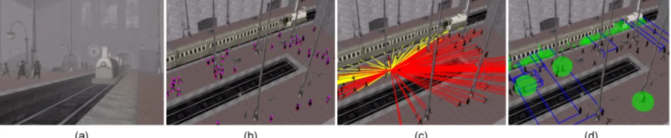
The techniques discussed above directly apply to audio rendering of complex, dynamic, 3D scenes containing numerous point sources. They also apply to rendering of extended sources, modeled as a collection of point sources such as the train in Figure 10. In this train station example with 160 sound sources, we were able to render both the visuals (about 70k polygons) and pre-mix the audio on the GPU (ATI Radeon mobility 5700 on a Compaq laptop). Pre-mixing with the CPU (Pentium4 mobility 1.8GHz), using a C++ implementation, resulted in degraded performance (i.e., reduced visual refresh) but improved audio quality. Perceptual criteria used for loudness evaluation, source culling and clustering were pre-computed on the input signals using three sub-bands (0-500 Hz,500-2000 Hz,2000+ Hz) and short audio frames of 1024 samples at 44.1kHz. For more information and technical details, we refer the reader to [36].
Figure 10 – (a) An application of the perceptual rendering pipeline to a complex train-station environment. (b) Each pedestrian acts as two sound sources (voice and footsteps). Each wheel of the train is also modeled as a point sound source to get the proper spatial rendering for this extended source. Overall, 160 sound sources must be rendered (magenta dots). (c) Colored lines represent direct sound paths from the sources to the listener. All lines in red represent perceptually masked sound sources while yellow lines represent audible sources. Note how the train noise masks the conversations and footsteps of the pedestrians. (d) Clusters are dynamically constructed to spatialize the audio. Green spheres indicate representative location of the clusters. Blue boxes are bounding boxes of all sources in each cluster.
Audio rendering was implemented using DS3D accelerated by the built-in SoundMax chipset (32 3D audio channels). A drawback of the approach is increased bus traffic, since the audio signals for each cluster are pre-mixed outside the APU and must be continuously streamed to the hardware channels. Also, since aggregate signals and representative location for each cluster are continuously updated at each audio frame to best-fit the current soundscape, care must be taken to avoid artefacts when switching the position of the audio channel with DS3D. Switching must happen in-sync with the playback of each new audio frame and can be implemented through the DS3D notification mechanism. On certain hardware platforms, perfect synchronization cannot be achieved but artefacts can be minimized by enforcing spatial coherence of the audio channels from frame to frame (i.e., making sure a channel is used for clusters whose representatives are as close to each other as possible).
View Example 5 : train-station rendered with GPU pre-mixing View Example 6 : train-station rendered with CPU pre-mixing
Another application that requires spatialization of numerous sound sources is the simulation of early reflected or diffracted paths from walls and objects in the scene [20,27]. Commonly used techniques, based on geometrical acoustics, use ray or beam tracing to model the indirect contributions as a set of virtual image-sources [14,27].
The number of image-sources grows exponentially with the reflection order, limiting such approaches to a few early reflections or diffractions (i.e., reaching the listener first). Obviously, this number further increases with the number of actual sound sources present in the scene, making this problem a perfect candidate for clustering operations.
Spatial audio bridges
Voice communication, as featured on the Xbox Live! system, adds a new dimension to massively multi-player on-line gaming but is currently limited to monaural audio restitution. Next generation on-line games or chat-rooms will require dedicated spatial audio servers to handle real-time spatialized voice communication between a large number of participants. The various techniques discussed in this paper can be implemented on a spatial audio server to dynamically build clustered representations of the soundscape for each participant, adapting the resolution of the process to the processing power of each client, server load and network load. In such applications, an adaptive clustering strategy could be used to drive a multi-resolution binaural cue coding scheme [35], compressing the soundscape and including incoming voice signals as a single or a small collection of monaural audio streams and corresponding time-varying 3D positional information. Rendering of the spatialized audio scene could be done either on the client side (if the client supports 3D audio rendering) or on the server side (e.g., if the client is a mobile device with low processing power).
Conclusions
We presented a set of techniques aimed at spatialized audio rendering of large numbers of sound sources with limited hardware resources. This techniques will hopefully simplify the work of the game audio designer and developer by removing limitations imposed by the audio rendering hardware. We believe these techniques can be used to leverage the capabilities of current audio hardware while enabling novel effects, such as the use of extended sources. They could also drive future research in audio hardware and audio rendering API design to allow for better rendering of complex dynamic soundscapes.
Acknowledgements
The author would like to thank Yannick Bachelart, Frank Quercioli, Paul Tumelaire, Florent Sacré and Jean-Yves Regnault for the visual design, modeling and animations of the train-station environment. Christophe Damiano and Alexandre Olivier-Mangon designed and modeled the various elements of the countryside environment. Some of the voice samples in the train-station example were originally recorded by Paul Kaiser for the artwork ”TRACE” by Kaiser and Tsingos. This work was partially funded by the 5th Framework IST EU project “CREATE” IST-2001-34231.
References and further reading
Game Audio Programming and APIs
[1] Soundblaster, © Creative Labs. http://www.soundblaster.com
[2] Direct X homepage, © Microsoft. http://www.microsoft.com/windows/directx/default.asp
[3] Environmental audio extensions: EAX © Creative Labs. http://www.soundblaster.com/eaudio, http://developer.creative.com
[4] EAGLE © Creative Labs. http://developer.creative.com
[5] ZoomFX, MacroFX, ©Sensaura. http://www.sensaura.co.uk
Books
[6] D.R. Begault. 3D Sound for Virtual Reality and Multimedia. Academic Press Professional, 1994.
[7] J. Blauert. Spatial Hearing : The Psychophysics of Human Sound Localization. M.I.T. Press, Cambridge, MA, 1983. [8] A.S. Bregman. Auditory Scene Analysis, The perceptual organization of sound. M.I.T Press, Cambridge, MA,1990.
[9] A. Gersho and R.M. Gray. Vector quantization and signal compression, The Kluwer International Series in Engineering and Computer
[10] K. Steiglitz. A DSP Primer with applications to digital audio and computer music. Addison Wesley, 1996. [11] E. Zwicker and H. Fastl. Psychoacoustics: Facts and Models. Springer, 1999.
[12] M. Kahrs and K. Brandenburg Ed., Applications of Digital Signal Processing to Audio and Acoustics, Kluwer Academic Publishers, 1998.
[13] David Luebke, Martin Reddy, Jonathan D. Cohen, Amitabh Varshney, Benjamin Watson, and Robert Huebner. Level of Detail for 3D
Graphics. Morgan Kaufmann Publishing. 2002
Papers
[14] J. Borish. Extension of the image model to arbitrary polyhedra. J. of the Acoustical Society of America, 75(6), 1984.
[15] K. Brandenburg. MP3 and AAC explained. AES 17th International Conference on High-Quality Audio Coding, September 1999. [16] D.P.W. Ellis. A perceptual representation of audio. Master’s thesis, Massachusets Institute of Technology, 1992.
[17] H. Fouad, J.K. Hahn, and J.A. Ballas. Perceptually based scheduling algorithms for real-time synthesis of complex sonic environments.
Proceedings of the 1997 International Conference on Auditory Display (ICAD’97), Xerox Palo Alto Research Center, Palo Alto, USA, 1997.
[18] P. Fränti, T. Kaukoranta, and O. Nevalainen. On the splitting method for vector quantization codebook generation. Optical Engineering, 36(11):3043–3051, 1997.
[19] P. Fränti and J. Kivijärvi. Randomised local search algorithm for the clustering problem. Pattern Analysis and Applications, 3:358 - 369, 2000.
[20] T. Funkhouser, P. Min, and I. Carlbom. Real-time acoustic modeling for distributed virtual environments. ACM Computer Graphics,
SIGGRAPH’99 Proceedings, pages 365–374, August 1999.
[21] J. Herder. Optimization of sound spatialization resource management through clustering. The Journal of Three Dimensional Images,
3D-Forum Society, 13(3):59–65, September 1999.
[22] J. Herder. Visualization of a clustering algorithm of sound sources based on localization errors. The Journal of Three Dimensional
Images, 3D-Forum Society, 13(3):66–70, September 1999.
[23] I.J. Hirsh. The influence of interaural phase on interaural summation and inhibition. J. of the Acoustical Society of America, 20(4):536– 544, 1948.
[24] A. Likas, N. Vlassis, and J.J. Verbeek. The global k-means clustering algorithm. Pattern Recognition, 36(2):451–461, 2003. [25] E. M. Painter and A. S. Spanias. A review of algorithms for perceptual coding of digital audio signals. DSP-97, 1997.
[26] R. Rangachar. Analysis and improvement of the MPEG-1 audio layer III algorithm at low bit-rates. Master thesis, Arizona State Univ., December 2001.
[27] N. Tsingos, T. Funkhouser, A. Ngan, and I. Carlbom. Modeling acoustics in virtual environments using the uniform theory of diffraction. ACM Computer Graphics, SIGGRAPH’01 Proceedings, pages 545–552, August 2001.
[28] W. Martens, Principal Components Analysis and Resynthesis of Spectral Cues to Perceived Direction, Proc. Int. Computer Music Conf.
(ICMC'87), pages 274-281, 1987.
[29] K. van den Doel, D. K. Pai, T. Adam, L. Kortchmar and K. Pichora-Fuller, Measurements of Perceptual Quality of Contact Sound Models, Proceedings of the International Conference on Auditory Display (ICAD 2002), Kyoto, Japan, pages 345-349, 2002.
[30] M. Lagrange and S. Marchand, Real-time Additive Synthesis of Sound by Taking Advantage of Psychoacoustics, Proceedings of the
COST G-6 Conference on Digital Audio Effects (DAFX-01), Limerick, Ireland, December 6-8 2001.
[31] V. Pulkki, Virtual Sound Source Positioning using vector Base amplitude panning, J. Audio Eng. Soc., 45(6), page 456-466, june 1997. [32] B. C. J. Moore and B. Glasberg and T. Baer, A Model for the Prediction of Thresholds, Loudness and Partial Loudness, J. Audio Eng.
Soc., 45(4) : 224-240, 1997.
[33] E. Wenzel, J. Miller, and J. Abel. A software-based system for interactive spatial sound synthesis. Proceeding of ICAD 2000, Atlanta, USA, april 2000.
[34] York University Ambisonics homepage. http://www.york.ac.uk/inst/mustech/3d_audio/ambison.htm
[35] C. Faller and F. Baumgarte, Binaural Cue Coding Applied to Audio Compression with Flexible Rendering, Proc. AES 113th
Convention, Los Angeles, USA, Oct. 2002.
[36] N.Tsingos, E. Gallo and G. Drettakis. Perceptual audio rendering of complex virtual environments, INRIA Technical Report # 4734, February 2003.