HAL Id: hal-02060595
https://hal.archives-ouvertes.fr/hal-02060595
Submitted on 7 Mar 2019
HAL is a multi-disciplinary open access
archive for the deposit and dissemination of
sci-entific research documents, whether they are
pub-lished or not. The documents may come from
teaching and research institutions in France or
abroad, or from public or private research centers.
L’archive ouverte pluridisciplinaire HAL, est
destinée au dépôt et à la diffusion de documents
scientifiques de niveau recherche, publiés ou non,
émanant des établissements d’enseignement et de
recherche français ou étrangers, des laboratoires
publics ou privés.
Reconfigurable transfer line balancing problem: A new
MIP approach and approximation hybrid algorithm
Y Lahrichi, L. Deroussi, Sylvie Norre, Nathalie Grangeon
To cite this version:
Y Lahrichi, L. Deroussi, Sylvie Norre, Nathalie Grangeon. Reconfigurable transfer line balancing
problem: A new MIP approach and approximation hybrid algorithm. MOSIM 2018 (Modélisation et
Simulation), Jun 2018, Toulouse, France. �hal-02060595�
Reconfigurable transfer line balancing problem: A new MIP
approach and approximation hybrid algorithm.
Y. LAHRICHI, L. DEROUSSI, N. GRANGEON, S. NORRE
LIMOS / CNRS UMR 6158 Campus Universitaire des C´ezeaux
1 rue de la Chebarde
63178 AUBIERE CEDEX - FRANCE [email protected]
ABSTRACT: We consider the problem of balancing reconfigurable transfer lines. The problem is quite recent and motivated by the growing need of reconfigurability in the new INDUSTRY 4.0 context. The problem consists into allocating different tasks necessary to machine a single part to different workstations placed into a serial line. The workstations can contain multiple machines operating in parallel and the tasks allocated to a workstation should be sequenced since the machines considered are mono-spindle head CNC machines and setup times between operations are needed to perform tool changes. Besides precedence constraints between operations are considered. In this article we suggested a new MIP approach based on formulation presented by Andr´es et al.(2008) for a resembling problem. We suggest effective pre-processing procedures and a new lower bound. We besides suggest a novel hybrid approach that approximate the optimal solution when the setup times are bounded by the completion times. Experimentation are performed on benchmark instances and the methods are compared with those suggested in the literature.
KEYWORDS: Transfer line balancing, Reconfigurability, Industry 4.0, Mixed integer programming, Hybrid algorithms, approximation algorithms
1 INTRODUCTION
New consuming trends, global competition and grow-ing variety in demand in the actual economical con-text raises an important issue in transfer line design. In fact, shortening life cycle times imposes the con-sideration of reconfigurabiliy in transfer line design. The modern transfer line should be easily and cost-effectively reconfigurable to address two different is-sues: the variability in production size and the vari-ability in the product specifications. While the first one imposes a variation in cycle time, the second one is linked to the set of tasks involved.
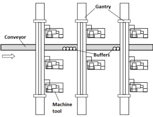
To address this issue, Koren et al.(1999) suggested in late 1990s the novel concept of Reconfigurable Manufacturing System (RMS). A RMS could be seen as a serial line of workstations (corresponding to the stages in Figure.1). Each workstation is equipped by multiple machines operating in parallel. Part units are moved from a workstation to another thanks to a conveyor. The part is delivered then to the first available machine in a workstation from the gantry. The RMS highly addresses the issue of production size variability. Indeed the ability to add or remove
Figure 1 – Reconfigurable Manufacturing System: [Koren 2010]
a machine in a workstation allows monitoring the cy-cle time with high granularity which is refereed to as scalability [Koren 2017]. Besides RMS offers a good trade off between productivity and flexibility while Dedicated Manufacturing System are highly produc-tive but very poorly flexible and Flexible Manufac-turing System highly flexible but very expensive and almost never profitable.
MOSIM18 - June 27-29, 2018 - Toulouse - France
address the issue of variability in product specifica-tions only if equipped with mono-spindle head ma-chines. Indeed, those machines can perform a huge set of operations, each machine being equipped with a tool magazine. To perform an operation, a machine needs a specific tool. Thus, setup times between op-erations must be considered in addition to operation times in order to perform tool changing.
Once equipped with mono-spindle head machines, RMS addresses both the production size and prod-uct specifications variability issues: whenever one or both of these elements comes to change, the manufac-turer can easily adjusts the production by performing a reconfiguration of the system which can be seen as the process of balancing the transfer line taking into consideration setup times and multiple parallel ma-chines at each workstation. Once this operation per-formed, machines are then added or removed from workstations if necessary, and machines are remotely configured to perform the new sequence of operations; RMS allowing to perform those two steps rapidly and cost-effectively. There is no need of physical machine reconfiguration, since all machines are equipped with the same tool magazine and can thereby perform the same set of operations.
The problem of balancing RMS appears then to be of strategic importance for the manufacturer. In section 2 we define this problem and introduce basic nota-tions, a lower bound and an example are introduced in section 3 then in section 4 the related work is de-scribed. A new MIP approach is presented in section 5 and a novel approximation hybrid algorithm is then introduced in section 6. An experimental study was also performed, it is showing highly promising results. It is covered in the section 7 of the paper.
2 PROBLEM DEFINITION
The instance of the optimization problem could be described by the following data:
• The set of operations, the corresponding times, setup times and precedence relations.
• A maximum number of workstations to be used placed serially.
• A maximum number of machines per worksta-tion.
• A cycle time.
• A maximum number of operations to be allo-cated to a workstation.
The optimization problem consists then in finding an allocation of the operations to the workstations and
determining a number of machines per workstation while minimizing the number of machines used and respecting the following constraints:
• The sum of the times of the operations and the induced setup times of the sequence allocated to a workstation divided by the number of machines in that workstation must not exceed the cycle time.
• Precedence constraints must be respected: when an operation i precedes an operation j, the work-station to which the operation i is allocated must be less (placed before in the line) or as the work-station to which the operation j is allocated. • The number of workstations must not exceed the
maximum number of workstations.
• The number of operations allocated to a work-station must not exceed the maximum number of operations per workstation.
• The number of machines in a workstation must not exceed the maximum number of machines per workstation.
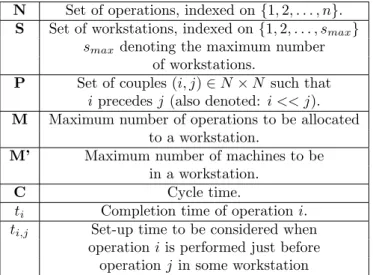
For the rest of the paper, we use the notations pre-sented in Table.1.
N Set of operations, indexed on {1, 2, . . . , n}. S Set of workstations, indexed on {1, 2, . . . , smax}
smaxdenoting the maximum number
of workstations.
P Set of couples (i, j) ∈ N × N such that i precedes j (also denoted: i << j). M Maximum number of operations to be allocated
to a workstation.
M’ Maximum number of machines to be in a workstation.
C Cycle time.
ti Completion time of operation i.
ti,j Set-up time to be considered when
operation i is performed just before operation j in some workstation
Table 1 – Table of notations.
3 RELATED WORK
This problem could be seen as an assembly line bal-ancing problem. Those problems have been well stud-ied in the literature; however those considering paral-lel machines or sequence dependent setup times have rarely been considered. The originality of the prob-lems comes from the consideration of both elements. We can only list two papers dealing with this issue
with an exact approach: (Essafi et al., 2010) and (Borisovsky et al., 2012 & 2014).
Both approaches fail to solve the problem for medium to large scale instances. Essafi et al.(2010) suggest a MIP approach while Borisovsky et al.(2014) uses a set partitioning model coupled with a constraint generation algorithm.
The MIP approach of Essafi et al. (2010) lies on mod-elling the overall sequence constituted of the concate-nation of the sequences of all the workstations :it uses the variables xi,q(i for the operation and q for the
po-sition in the sequence). It can solve instances with 15 operations while the other approach (Borisovsky et al., 2014) can solve instances with up to 50 opera-tions.
4 EXAMPLE AND LOWER BOUND We first introduce a new lower bound for the problem, we then draw an example and its optimal solution. Taking into consideration the fact that for every workstation j, its workload time (Wj) and its number
of machines mj should satisfy:
Wj ≤ C.mj
Then, the total workload W =P
j∈SWj and the
to-tal number of machines m =P
j∈Smj must satisfy: W =X j∈S Wj≤ X j∈S C.mj = C. X j∈S mj = C.m i.e: W ≤ C.m (1)
Let us now assume that n > smax. Then the workload
W must satisfy: W ≥X
i∈N
ti+ λ1+n−smax (2)
where λ1+n−smax denotes the 1 + n − smax smallest
setup times.
Indeed, (2) is true because the workload is composed of the operations times (P
i∈Nti) and the induced
setup times. And since n > smax, there must be at
least n − smaxoperations that are ”not alone” at the
workstation they are affected to. Any solution must then consider at least n − smax+ 1 setup times. (+1
because a sequence of k operations induce exactly k setup times)
Then, we have from (1) and (2): X
i∈N
ti+ λ1+n−smax≤ C.m
From this equation we deduce a new lower bound for the number of machines used if n > smax:
zlb= & P i∈Nti+ λ1+n−smax C ' (3)
If n ≤ smax, the classical lower bound for SALBP is
still available : zlb= & P i∈Nti C '
Let us know give the example of a small instance, compute the lower bound and give an optimal solu-tion.
The instance is described by the following data:
• The part requires the execution of 7 operations numbered from 1 to 7 (n = 7).
• At most 3 stations can be used. (smax= 3).
• Precedence constraints are given by:
P = {(1, 3), (2, 3), (3, 4), (4, 5), (5, 6), (5, 7)} represented in Figure.2. 3 1 2 4 5 6 7
Figure 2 – Precedence graph.
• M = 3, Maximum number of operations that could be allocated to a workstation.
• M0 = 3, Maximum number of machines that
could be hosted by a workstation.
• Completion times are represented in Table.2: i 1 2 3 4 5 6 7 ti 1.5 1 3.5 1.5 2.5 3 1
Table 2 – Operations times.
• Setup times are represented in Table.3. • C = 2.5, cycle time.
MOSIM18 - June 27-29, 2018 - Toulouse - France ti,j j = 1 2 3 4 5 6 7 i = 1 X 0.5 10 10 10 10 10 2 10 X 0.5 10 10 10 10 3 0.5 10 X 10 10 10 10 4 10 10 10 X 0.5 10 10 5 10 10 10 0.5 X 10 10 6 10 10 10 10 10 X 0.5 7 10 10 10 10 10 0.5 X
Table 3 – Setup times.
Computing the lower bound (equation 3) gives: zlb=
7.
We describe a realizable solution by allocating to the first workstation the sequence 1, 2, 3 and 3 machines, to the second workstation the sequence 4, 5 and 2 ma-chines and to the third workstation the sequence 6, 7 and 2 machines.
The solution is realizable since the workload divided by the number of machines for each station does not exceed the cycle time:
For station 1:(t1+ t2+ t3+ t1,2+ t2,3+ t3,1)/3 = 2.5
For station 2:(t4+ t5+ t4,5+ t5,4)/2 = 2.5
For station 3:(t6+ t7+ t6,7+ t7,6)/2 = 2.5
Since the solution is realizable and its cost equals the lower bound, it is optimal.
5 A MIP FORMULATION AND PRE-PROCESSING PROCEDURES
In this section, we describe a new MIP approach based on a formulation for the sequence-dependent setup times assembly line balancing problem intro-duced by Andr´es et al.(2008) that has not been experimented and does not consider parallel ma-chines in workstations. Besides we suggest novel pre-processing procedures that computes:
• ei: The earliest station to which operation i
could be affected.
• li: The latest station to which operation i could
be affected.
• Mj: The maximum number of operations that
could be affected to workstation j.
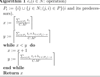
We first give the pre-processing algorithms, we then describe the MIP approach for our problem.
While x denotes the earliest station to ensure that the workload of i and all its predecessors is done, the condition x < y captures the fact that x stations are
Algorithm 1 ei(i ∈ N : op´eration)
Pi := {i} ∪ {j ∈ N ; (j, i) ∈ P }(i and its
predeces-sors). x := & P i∈Piti C.M0 ' y := & P i∈Piti+λ1+|Pi|−x C.M0 ' while x < y do x := x + 1 y := & P i∈Piti+λ1+|Pi|−x C.M0 ' end while Return x
not enough to ensure that the induced setup times are also processed. The second algorithm computing the latest workstation is quite similar to the first one but considering the successors instead of predecessors and counting from smax in stead of 1.
Algorithm 2 li(i ∈ N : op´eration)
Si:= {i} ∪ {j ∈ N ; (i, j) ∈ S}(i and its successors).
x := & P i∈Siti C.M0 ' y := & P i∈Siti+λ1+|Si|−x C.M0 ' while x < y do x := x + 1 y := & P i∈Siti+λ1+|Si|−x C.M0 ' end while Return smax− x + 1
Once having computed ei and li, we could
re-view the maximum number of operations that could be affected to any workstation j as: Mj =
M in(M, |{i, ei≤ j ≤ li, i ∈ N }|).
Another pre-processing procedure is run to remove redundant precedence constraints : (i, j) ∈ P is re-moved if there exists a non trivial path between i and j in the precedence graph.
We could now describe the MIP approach. This ap-proach is based in modelling the workstations se-quences. It uses the following binary variables:
• xi,j,s= 1 If operation i is affected to workstation j in the sth
position of its sequence. 0 If not.
•
yj=
1 If at least one operation is affected to workstation j 0 If not. • zi,j,k=
1 If the operation i is processed just before operation j at workstation k. 0 If not. • wi,j=
1 If the operation i is affected to the last position of workstation j. 0 If not. • vj,k=
1 If k machines are affected to workstation j.
0 If not.
We consider the objective of minimizing the number of machines used: M inP j∈S PM0 k=1k.vj,k under the constraints: l(i) X j=e(i) Mj X s=1 xi,j,s= 1, ∀i ∈ N (4)
This set of constraints ensures that every operation is affected to exactly one workstation at a unique po-sition of its sequence.
X
i∈N,e(i)≤j≤l(i)
xi,j,s≤ 1, ∀j ∈ S, s = 1, ..., Mj (5)
This set of constraints ensures that at most one oper-ation is affected to each position of the sequences of the workstations. X i∈N,e(i)≤j≤l(i) xi,j,s+1≤ X i∈N,e(i)≤j≤l(i) xi,j,s ∀j ∈ S, s = 1, ..., mj− 1 (6)
This set of constraints ensures that no position s + 1 in any workstation is taken by any operation unless the position s is also taken by some operation.
M0
X
k=1
vj,k= yj, ∀j ∈ S (7)
This set of constraints ensures that only one number of machines is chosen for every used workstation.
yj+1≤ yj, ∀j = 1, ..., smax− 1 (8)
This set of constraints ensures that no workstation is used unless its precedent workstation is also used.
l(i) X j=e(i) Mj X s=1 (M.(j − 1) + s)xi,j,s≤ l(i0) X j=e(i0) Mj X s=1 (M.(j − 1) + s)xi0,j,s∀(i, i0) ∈ P (9)
This set of constraints ensure that precedence con-straints are satisfied.
X i∈N,e(i)≤j≤l(i) Mj X s=1 ti.xi,j,s+ X
i,i0∈N2;i6=i0,e(i)≤j≤l(i),e(i0)≤j≤l(i0)
ti,i0.zi,i0,j ≤ C. M0 X k=1 k.vj,k, ∀j ∈ S (10)
This set of constraints ensure that the cycle time is not exceeded in any workstation.
xi,k,s+ xi0,k,s+1≤ 1 + zi,i0,k, ∀i, i0 ∈ N2, i 6= i0,
k ∈ {e(i), ..., l(i)} ∩ {e(i0), ..., l(i0)}, s = 1, ..., mk− 1
(11) This set of constraints ensures that if operation i0 is followed by operation i zt station k then zi,i0,k is put
to 1. xi,j,s− X i0∈N ;i06=i,e(i0)≤j≤l(i0) xi0,j,s+1≤ wi,j, ∀i ∈ N, ∀j ∈ {e(i), ..., l(i)}, s = 1, ..., mj− 1 (12)
xi,j,Mj ≤ wi,j, ∀i ∈ N, ∀j ∈ {e(i), ..., l(i)} (13)
The constraints (13) and (14) ensure that wi,j is put
to one whenever operation i is positioned in the last occupied position of workstation j.
wi,j+ xi0,j,1≤ 1 + zi,i0,j, ∀i ∈ N, i0∈ N, i 6= i0,
j ∈ {e(i), ..., l(i)} ∩ {e(i0), ..., l(i0)} (14) This constraint ensures that if operation i is posi-tioned in the last occupied position of workstation j and operation i0 positioned in the first position of workstation j then zi,i0,j = 1 and consequently the
setup time ti,i0 is considered in (10).
MOSIM18 - June 27-29, 2018 - Toulouse - France
6 AN HYBRID APPROACH
Let’s now describe a novel hybrid approach for our problem. Besides, we show that the algorithm is a 2-approximation if we assume that:
ti,j≤ tk, ∀i, j, k ∈ N (15)
which seems to be a very reasonable and realistic as-sumption while considering industrial instances. (see section.7)
The algorithm consists of two steps. The first consists of solving a MIP while the second one is an exact dy-namic programming algorithm for solving the ATSP:
• Step 1 : Perform a parallel line balancing with-out taking setup times into consideration using a MIP approach.
• Step 2 : For each workstation, perform a sequenc-ing of the operations ussequenc-ing a dynamic program-ming algorithm then if the number of machines in the workstations is insufficient to fulfill the cycle time, add the necessary ones. If the maximum number of machines is violated, then we return to step 1 by adding a constraint that forbids the assignment of the set of operations to the work-station. This step is described in more details in section 6.2.
The first subsection is devoted to the first step and the second subsection is devoted to the second step.We refer to this method as ”BFSL” (Balance First, Se-quence Last )
Let us now remark that the solution outputted by the algorithm is feasible and its overall cost (c) is given by the cost of the solution outputted by the step1 (c1) plus the number of machines added in step 2 (m). i.e
c = c1+ m
besides we have c1≤ c∗where c∗denotes the optimal
solution of the RMS balancing problem (because c1
does not take setup times into consideration). And thanks to (15) we have m ≤ c1 (because the
number of setup times for each workstation is less or equal to the number of operations and then the workload involved by the setup times in each work-station is less or equal to the workload involved by the operations times). Those two inequations (c1 ≤ c∗,
m ≤ c1) finally give:
c ≤ 2.c∗
which shows the approximation ratio.
6.1 Step 1: Balancing without setup times In this step we are concerned with balancing the RMS but without taking into consideration setup-times. This is done by the following MIP that is derived from the precedent one by removing unnecessary variables and constraints. We use the following variables:
xi,j= 1 If operation i is affected to workstation j. 0 If not. yj =
1 If at least one operation is affected to workstation j 0 If not. vj,k=
1 If k machines are affected to workstation j.
0 If not.
We consider the objective of minimizing the number of machines used: M inP
j∈S
PM0
k=1k.vj,k
under the constraints:
l(i)
X
j=e(i)
xi,j= 1, ∀i ∈ N (16)
This set of constraints ensures that every operation is affected to exactly one workstation.
M0
X
k=1
vj,k= yj, ∀j ∈ S (17)
This set of constraints ensures that only one number of machines is chosen for every used workstation.
X
i∈N,e(i)≤j≤l(i)
xi,j ≤ Mj, ∀j ∈ S (18)
This set of constraints ensures that the maximum number of operations to be allocated to a worksta-tion is respected.
yj+1≤ yj, ∀j = 1, ..., smax− 1 (19)
This set of constraints ensures that no workstation is used unless its precedent workstation is also used.
l(i) X j=e(i) j.xi,j≤ l(i0) X j=e(i0) j.xi0,j, ∀(i, i0) ∈ P (20)
This set of constraints ensures that precedence con-straints are satisfied.
X i∈N,e(i)≤j≤l(i) ti.xi,j≤ C. M0 X k=1 k.vj,k, ∀j ∈ S (21)
This set of constraints ensures that the cycle time is not exceeded in any workstation.
The above MIP introduces far less variables and con-straints that the first MIP. Experimentation show that it can solve instances with very large set of op-erations.
6.2 Step 2: Sequencing operations in every workstation and adding necessary ma-chines
From step 1, we are given the affectation of opera-tions to the workstaopera-tions with a number of machines at each workstation. We are now concerned with sequencing the operations in every workstation and since the setup times were not considered in step 1 we may be obliged to add some machines at some workstations to fill the cycle time constraint.
The sequencing problem is an ATSP where opera-tions represent cities and set-up times distances be-tween cities. This operation is performed with an exact dynamic programming algorithm introduced in Held and Karp (1962). We compute then the work-load for every workstation and determine easily the number of machines to be added. If more machines than the the maximum authorized is required then we return to step 1 and a constraint forbidding the allocation of this set of operations to the workstation is added to the linear model.
7 EXPERIMENTAL RESULTS
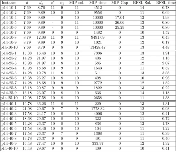
We describe in this section the experimentation be-ing held on a 16Go RAM computer with JAVA 8 and CPLEX (v12.7.0). Three sets of instances are considered, provided by Borisovsky et al.(2014) and described to be of industrial importance. However those instances consider additional constraints: ac-cessibility, inclusion and exclusion. Those constraints are taken into consideration by adding the necessary linear constraints. Experimentation are summarized in Table.4. z∗ and z denote respectively the opti-mal solution and the lower bound. ”MIP sol.” denote the solution outputted by CPLEX after ”MIP time” seconds. If the optimal solution is not found after 10,000 seconds, CPLEX is stopped and the actual best known solution is taken with its corresponding duality gap. d denotes the density of the precedence graph while dsdenotes the Scholl density:
ds =
2∗100∗P
i∈N|Pi|
n∗(n−1) where Pi denotes the
predeces-sors of i.
”BFSL” and ”BFSL time” denote respectively the so-lution and the time of the hybrid approach.
First set of instances (p14-10) have a Scholl density
in [5,15]. 6 instances out of 10 have been solved to optimum. With the MIP from Essafi et al.(2010) only 4 out of 10 instances have been solved to optimum with a time limit of 10,000 seconds. Second set of instances (p14-25) have a Scholl density in [15,25]. All instances have been solved to optimum. With the MIP from Essafi et al.(2010) only 5 out of 10 instances have been solved to optimum with a time limit of 10,000 seconds. Third set of instances (p14-40) have a Scholl density in [25,40]. All instances have been solved to optimum. With the MIP from Essafi et al.(2010) only 8 out of 10 instances have been solved to optimum with a time limit of 10,000 seconds. The MIP was enable to solve instances with 20 oper-ations within 10,000 seconds. All the instances were solved by the set partitioning model, besides the set partitioning model was able to solve instances with 50 operations.
8 CONCLUSION AND PERSPECTIVES We can make some remarks from the experimenta-tion:
• The MIP is more efficient with instances having bigger Sholl density.
• The lower bound that we present is on average at 15% of the optimal solution.
• The hybrid approach gives medium results and is very fast. The approximation ratio is satisfied. A posterior local search improvement step would be an interesting perspective.
• The MIP that we present is more efficient than the one presented in Essafi et al.(2010) and less efficient than the algorithm presented in Borisovsky et al.(2014).
We have presented in this paper a new MIP, and a novel hybrid approximation algorithm and held ex-perimentation on both Benchmark and randomly gen-erated instances. The results are quite promising. However, we could take many directions as a con-tinuation of this research:
• Improvement of the BFSL algorithm with pos-terior local search improvement algorithms for example.
• The use of polyhedral approaches lying on the MIP.
• Research could be done to show a better approx-imation ratio if there exists some λ ∈ [0, 1] s.t:
MOSIM18 - June 27-29, 2018 - Toulouse - France
Instance d ds z∗ zlb MIP sol. MIP time MIP Gap BFSL Sol. BFSL time
p14-10-1 7.69 8.76 11 9 11 4512 0 14 0.78 p14-10-2 7.69 9.89 10 8 10 9558 0 11 0.69 p14-10-4 7.69 9.89 - 9 10 10000 17.04 12 1.93 p14-10-5 7.69 9.89 - 8 11 10000 26.06 13 0.80 p14-10-6 7.69 9.89 - 8 11 10000 25.29 13 0.80 p14-10-7 7.69 9.89 9 8 9 1482 0 10 1.52 p14-10-8 8.79 12.08 11 9 11 9491.69 0 13 0.43 p14-10-9 8.79 9.89 10 9 10 1021 0 12 0.17 p14-10-10 7.69 8.79 9 8 9 13428.47 0 13 4.48 p14-25-1 15.38 16.48 10 8 10 7336 0 13 1.91 p14-25-2 14.28 21.97 10 8 10 406 0 12 1.18 p14-25-3 10.98 21.97 10 8 10 585 0 12 2.07 p14-25-4 10.98 18.68 10 9 10 1543 0 11 0.52 p14-25-5 14.28 19.78 11 8 11 511 0 13 3.86 p14-25-6 15.38 25.27 10 8 10 498 0 10 0.96 p14-25-7 14.28 18.68 10 9 10 2772 0 12 1.82 p14-25-8 13.18 20.87 9 9 9 1822 0 13 0.22 p14-25-9 13.18 23.07 10 8 10 636 0 14 1.18 p14-25-10 12.08 17.58 10 8 10 2658 0 11 1.38 p14-40-1 19.78 36.26 11 8 11 229 0 13 1.31 p14-40-2 21.98 29.67 9 7 9 1778.32 0 12 0.93 p14-40-3 17.58 24.17 10 8 10 4006 0 12 0.41 p14-40-4 18.68 29.67 10 8 10 322 0 11 0.72 p14-40-5 14.28 26.37 10 8 10 838 0 12 1.78 p14-40-6 17.58 38.46 10 8 10 104 0 11 1.22 p14-40-7 17.58 26.37 9 7 9 1368 0 11 0.39 p14-40-8 19.78 26.37 9 8 9 491 0 11 0.40 p14-40-9 16.48 27.47 10 8 10 333.97 0 12 1.32 p14-40-10 16.48 29.67 9 8 9 409 0 10 0.41
Table 4 – Experimentation with benchmark instances.
• It will be more relevant to compare the hybrid approach with the approximate methods rather than the exact methods.
• Studying the problem in an uncertain context is a must to fill with INDUSTRY 4.0 requirements.
ACKNOWLEDGMENTS
The authors acknowledge the support received from the Agence Nationale de la Recherche of the French government through the program ”Investissements d’Avenir”(16-IDEX-0001 CAP 20-25).
REFERENCES
Andr´es, C., M. Crist´obal, and R. Pastor, 2008. Bal-ancing and scheduling tasks in assembly lines with sequence-dependent setup times. European Journal of Operational Research, Vol.187, No. 3, pp. 1212-1223.
Borisovsky, P. A., Delorme, X., and A. Dolgui, 2014. Balancing reconfigurable machining lines by means of set partitioning model. Interna-tional Journal For Production Research, Vol. 52,
pp. 4026-4036.
Essafi, M., X. Delorme X., A. Dolgui A., and O. Guschinskaya, 2010. A MIP approach for bal-ancing transfer line with complex industrial con-straints. CIRP Journal of Manufacturing Sci-ence and Technology, Vol. 58, No.2, pp. 176-182. Held, M., and R. M. karp. 1962. A Dynamic Pro-gramming Approach to Sequencing Problems. Journal of the Society for Industrial and Applied Mathematics, Vol.10, pp. 196-210.
Koren, Y., U. Heisel, F. Jovane, T. Moriwaki, G. Pritschow, G. Ulsoy, and H. Van Brussel, 1999. Economic benefits of reconfigurable manufactur-ing systems. Annals of CIRP, Vol. 42, No. 2, pp. 527-540.
Koren, Y., 2010. The global manufacturing revolu-tion - product-process-business integrarevolu-tion and reconfigurable systems. John Wiley & Sons. Wang, W., Y. Koren, and X. Gu, 2017. Value
creation through design for scalability of recon-figurable manufacturing systems. International Journal For Production Research, Vol. 55, No. 5, pp. 1227-1242.