Spatial Holmboe instability

HAL Id: hal-00830698

https://hal-ensta-paris.archives-ouvertes.fr//hal-00830698

Submitted on 3 Sep 2014

HAL is a multi-disciplinary open access

archive for the deposit and dissemination of

sci-entific research documents, whether they are

pub-lished or not. The documents may come from

teaching and research institutions in France or

abroad, or from public or private research centers.

L’archive ouverte pluridisciplinaire HAL, est

destinée au dépôt et à la diffusion de documents

scientifiques de niveau recherche, publiés ou non,

émanant des établissements d’enseignement et de

recherche français ou étrangers, des laboratoires

publics ou privés.

Spatial Holmboe instability

Sabine Ortiz, J.-M. Chomaz, Thomas Loiseleux

To cite this version:

Sabine Ortiz, J.-M. Chomaz, Thomas Loiseleux. Spatial Holmboe instability. Physics of Fluids,

American Institute of Physics, 2002, 14 (8), pp.2585-2597. �10.1063/1.1485078�. �hal-00830698�

Sabine Ortiz, Jean-Marc Chomaz, and Thomas Loiseleux

Citation: Physics of Fluids (1994-present) 14, 2585 (2002); doi: 10.1063/1.1485078 View online: http://dx.doi.org/10.1063/1.1485078

View Table of Contents: http://scitation.aip.org/content/aip/journal/pof2/14/8?ver=pdfcov

Published by the AIP Publishing

Articles you may be interested in

Optimal excitation of two dimensional Holmboe instabilities

Phys. Fluids 23, 074102 (2011); 10.1063/1.3609283

Coupling of Kelvin–Helmholtz instability and buoyancy instability in a thermally laminar plasma

Phys. Plasmas 18, 022110 (2011); 10.1063/1.3555526

Secondary circulations in Holmboe waves

Phys. Fluids 18, 064104 (2006); 10.1063/1.2210504

On Holmboe’s instability for smooth shear and density profiles

Phys. Fluids 17, 084103 (2005); 10.1063/1.2001567

Symmetric and nonsymmetric Holmboe instabilities in an inviscid flow

Phys. Fluids 11, 1459 (1999); 10.1063/1.870009

ARTICLES

Spatial Holmboe instability

Sabine Ortiz

LadHyX, CNRS-Ecole Polytechnique F-91128 Palaiseau Cedex, France

and UME/DFA, ENSTA, chemin de la Hunie`re, F-91761 Palaiseau Cedex, France Jean-Marc Chomaz

LadHyX, CNRS-Ecole Polytechnique F-91128 Palaiseau Cedex, France Thomas Loiseleux

LadHyX, CNRS-Ecole Polytechnique F-91128 Palaiseau Cedex, France

and UME/DFA, ENSTA, chemin de la Hunie`re, F-91761 Palaiseau Cedex, France

共Received 26 February 2001; accepted 19 April 2002; published 18 June 2002兲

In mixing-layers between two parallel streams of different densities, shear and gravity effects interplay; buoyancy acts as a restoring force and the Kelvin–Helmholtz mode is known to be stabilized by the stratification. If the density interface is sharp enough, two new instability modes, known as Holmboe modes, appear, propagating in opposite directions. This mechanism has been studied in the temporal instability framework. The present paper analyzes the associated spatial instability problem. It considers, in the Boussinesq approximation, two immiscible inviscid fluids with a piecewise linear broken-line velocity profile. We show how the classical scenario for transition between absolute and convective instability should be modified due to the presence of propagating waves. In the convective region, the spatial theory is relevant and the slowest propagating wave is shown to be the most spatially amplified, as suggested by intuition. Predictions of spatial linear theory are compared with mixing-layer关C. G. Koop and F. K. Browand, J. Fluid Mech. 93, 135共1979兲兴 and exchange flow 关G. Pawlak and L. Armi, J. Fluid Mech. 376, 1 共1999兲兴 experiments. The physical mechanism for Holmboe mode destabilization is analyzed via an asymptotic expansion that predicts the absolute instability domain at large Richardson number. © 2002 American Institute of Physics. 关DOI: 10.1063/1.1485078兴

I. INTRODUCTION

Statically stable stratified shear layers have been widely documented due to their interest in geophysical and indus-trial situations. In the strait of Gibraltar, a stratified shear flow is generated between the heavier hot and salty water exiting the Mediterranean sea and the lighter cold Atlantic water entering into the sea共Armi and Farmer1兲. The Strait of Gibraltar is a prominent location where exchange flows natu-rally exist. A similar flow, called wedge flow, exists in fjords or in estuaries when fresh water enters the ocean space 共Paw-lak and Armi,2Farmer and Freeland3兲. Stratified shear flows also arise in atmospheric or oceanographic gravity currents resulting from the transient encounter of fluid masses with different densities, e.g., sea or mountain breezes, katabatic winds,4 snow avalanches or turbidity currents on the ocean floor 共Simpson5兲. In all these situations, instabilities are known to develop at the interface between the different fluid streams and to control the mixing that occurs at the interface. Miles6and Howard7have proven that stability of an inviscid continuous stratified flow is assured if the gradient Richard-son number, R_i(y )⫽⫺关g/(␳(dU/dy )2)兴(d␳/dy ) 关where g represents the gravity, ␳ the density, U(y ) the velocity as a

function of the vertical coordinate y兴 which compares locally buoyancy forces to inertia, is everywhere greater than 1/4. This result has been generalized by Yih8who shows that the same criterion holds when density discontinuities are present. However, Howard and Maslowe9 have shown that stratification effects are, in general, more complex since stable stratification adds a restoring force that constrains the vertical displacement of particles, and the instability depends on the details of the velocity and density profiles. A large research effort has been devoted to understanding the effect of buoyancy forces on shear instability by laboratory experiments,10–12 numerical studies,13,14 and theoretical analysis.15Based upon the totality of these numerical or the-oretical studies, which have focused on primarily temporal stability of the stratified shear flows, we know9 that if the characteristic thicknesses of the velocity shear and density interface are similar, the instability is stationary with respect to the mean flow, as in homogeneous flow, and is called Kelvin–Helmholtz instability. For a piecewise velocity pro-file and a two-layer step density model Holmboe16has found theoretically that the shear layer is primarily unstable either to Kelvin–Helmholtz waves or to two traveling waves, one moving upstream and the other downstream with respect to

PHYSICS OF FLUIDS VOLUME 14, NUMBER 8 AUGUST 2002

2585

1070-6631/2002/14(8)/2585/13/$19.00 © 2002 American Institute of Physics

the mean speed of the shear layer. In contrast to Kelvin– Helmholtz modes, those traveling modes called Holmboe modes17 in the inviscid approximation, are not restabilized when the stratification increases. Browand and Wang17 brought experimental evidence of the existence of Holmboe waves using a stratified water channel. Considering the ini-tial development, they measured the temporal amplification rates and found a fair agreement on the location of the neu-tral curve predicted by linear theory.16 Downstream evolu-tion of the perturbaevolu-tions has been reported by Browand and Winant.10 When the bulk Richardson number共value of the gradient Richardson number at y⫽0兲 is low enough, Kelvin–Helmholtz waves develop, roll up and break. When the bulk Richardson number is increased, the roll up is in-hibited and the interface starts being deformed by waves traveling in opposite directions, which form peaks protruding into the upper and lower layer. Numerical simulations of a temporally evolving stratified mixing-layer by Smyth, Klas-sen, and Peltier18 have substantiated both the breaking of Kelvin–Helmholtz waves and the development of both trav-eling waves. Assuming hyperbolic tangent velocity and den-sity profiles, Hazel13has studied the stability as a function of the ratio of the scale of the shear thickness to the density interface thickness. He shows applying the Miles–Howard criterion6,7that a ratio greater than two is a necessary condi-tion for instability whatever the value of the bulk Richardson number. However, appreciable growth rates for the Holmboe modes are numerically observed for a ratio greater than 2.5.18

Previous analysis was focused upon the temporal insta-bility of a stratified shear flow. However, in each field or laboratory situation a reference frame is singled out by boundary conditions and therefore, one should refer to the concept of absolute or convective instability to understand the dynamics of the flow共see Huerre and Monkewitz19for a review兲. Convectively unstable flows are known to behave as noise amplifiers and their dynamics are described by the spa-tial theory. In contrast, absolutely unstable flows exhibit self-sustained oscillations even in the absence of external pertur-bations, since the zero group velocity wave is amplified in the selected frame. For exchange flows, the frame is given by the earth since the flow is in the mean, stationary in this frame. For gravity currents, the selected frame will move with the head of the gravity current that sets up the shear flow. In laboratory mixing-layer facilities, the frame which is singled out is defined by the splitter plate at the end of which the two different fluids streams are set in contact. Studies of the absolute or convective instability in stratified sheared flows are not extensive in the literature and limited to cases where the only primary instability is stationary 共i.e., when the shear and density thicknesses are identical兲. This case has been studied by Lin and Pierrehumbert20and Triantafyllou.21 Only recently has the spatial stability theory been addressed by Pawlak and Armi22 in the case of wedge flow where the upper stream is assumed to be at rest, in which the scale of the density stratification is smaller than the scale of the shear and for small bulk Richardson number. They clearly demon-strate that the spatial theory differs strongly from the tempo-ral theory. The most amplified modes are different and the

spatial instability results from a combination of Kelvin– Helmholtz and Holmboe instabilities. However, they have addressed neither the effect of the mean advection nor the systematic study of the variations with the Richardson num-ber.

The purpose of the present paper is to extend Pawlak and Armi22 analysis to cases where the velocity of both streams are varied independently. Velocities may be in the same di-rection as in the mixing-layer or in opposite didi-rections as in exchange flows. On a model profile, we will systemati-cally determine the domain where the instability is absolute and where resonances are supposed to occur, varying the mean flow and the bulk Richardson number. This allows us to discuss the absolute and convective transitions for propa-gating modes. A similar case has been encountered in binary fluid mixtures,23 but in the present case the mean advection is not zero and the discussion is more complex than for binary convection. When the instability is convective, spatial growth rates will be determined. We will discriminate between flows where Kelvin–Helmholtz waves are stable and only the two Holmboe waves are unstable 共a case not treated by Pawlak and Armi22兲 and cases where the three modes are simultaneously unstable and interact. An asymptotic analysis will allow us to identify the physical mechanism that leads to the destabilization of Holmboe waves and will explain the domain of absolute instability associated to those waves. Finally, we will compare the present theory to field and laboratory experiments and pro-pose some predictions of the present model that might be easily tested in new experiments.

II. THE MODEL AND THE LINEAR DISPERSION RELATION

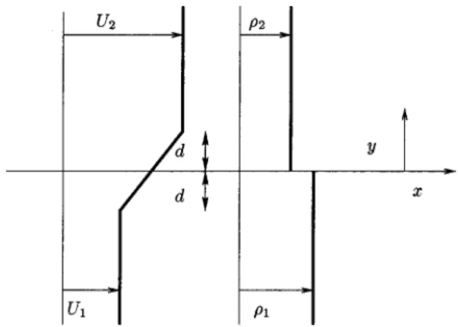
As sketched in Fig. 1, we consider two immiscible, in-viscid fluids of constant densities ␳1 and␳2 (␳1⬎␳2) under

the Boussinesq approximation共see Drazin and Reid,24p. 35兲. The layers are considered infinite and surface tension effects are neglected. The index 1 共resp. 2兲 denotes the lower layer

共resp. the upper layer兲. The dimensionless variables are

based on half the vorticity thickness d, half the shear inten-FIG. 1. Velocity and density profiles. An abrupt change in density occurs at the density interface; it is located at y⫽0. Abrupt changes in velocity gra-dient dU/dz defined the vorticity interfaces located at y⫽⫾d.

sity ⌬U⫽(兩U2⫺U1兩)/2, and the mean density (␳1⫹␳2)/2.

The mean velocity is defined by Um⫽(U1⫹U2)/2. The

den-sity interface is located at y⫽0 and the diffusive layer for the stratifying agent 共salt or temperature兲 is supposed infinitely thin for all time 共immiscible approximation兲. In our model, the gradient Richardson number 共see Drazin and Reid,24 p. 323兲, Ri(y )⫽⫺关g/(␳(dU/d y )2)兴(d␳/d y ) has a Dirac

func-tion behavior at y⫽0, and is not useful. This flow is charac-terized in terms of the bulk Richardson number Ri⫽关(␳1

⫺␳2)/(␳1⫹␳2)兴gd/⌬U2, which will be referred for

sim-plicity Richardson number. The flow is also defined by the dimensionless mean advection that will be useful only in the spatial theory

a⫽ Um

⌬U. 共1兲

Considering the stability of two-dimensional parallel flows for three-dimensional disturbances, Yih,25generalized Squire theorem,24without neglecting variations of density or viscos-ity, which may be continuous or discontinuous, he concluded that the fastest growing mode is two-dimensional. Therefore, we restrict our attention to two-dimensional perturbations of the stream function which are decomposed into normal modes of the form␾(y )exp(ik(x⫺ct)), where the eigenfunc-tion ␾ is governed by Rayleigh’s equation, k denotes the dimensionless wave number and c the phase velocity. In or-der to ensure that the perturbations decay at infinity␾(y ) is chosen at y→⫾⬁ to be of the form exp(⫾sky)(⫹ for y

→⫺⬁,⫺ for y→⫹⬁), where s⫽sgn(kr)共kris the real part

of k兲. Imposing the continuity of displacement and pressure at the vorticity and density interfaces give dispersion relation

共cf. Drazin and Reid,24_{or Pouliquen, Chomaz, and Huerre}26_兲

between k and␻⫽kc, the frequency of the wave

D共k,␻;Ri,a兲⫽共␻⫺ak兲4⫹n2k2共␻⫺ak兲2⫹n0k4⫽0, 共2兲 where n2⫽ ⫺Ri sk ⫹ e⫺4sk⫺共2sk⫺1兲2 4k2 and 共3兲 n0⫽ R_i sk 共e⫺2sk_{⫹2sk⫺1兲}2 4k2 , with s⫽sgn共kr兲. 共4兲 III. TEMPORAL INSTABILITY

The temporal instability theory considers waves homo-geneous in space (k苸R) which develop in time 共␻苸C, ␻

⬅␻r⫹i␻i兲. It correctly describes tilted tank experiments 共Thorpe,27_{Pouliquen, Chomaz, and Huerre}26_{兲 where two}

lay-ers of fluid initially at rest in a horizontal layer are set into relative motion by tilting the tank. We find an expression for the roots of共2兲 as follows:

␻⫽ak⫾

再

⫺n2k 2_⫾⌬1/2 2

冎

1/2 , 共5兲 with ⌬⫽共n2k2兲2⫺4n0k4. 共6兲

The mean advection a 关Eq. 共1兲兴 in the temporal case acts only as a Doppler shift in frequency, as shown in Eq.共5兲 and it affects only the real part of ␻ in the temporal theory. Therefore, temporal instability will be fully described by considering the intrinsic frequency of the temporal mode, defined as the frequency of the wave seen by an observer moving with the local mean flow␻_r*_{⫽␻r⫺ak as a function}

of k. Furthermore, since 共5兲 is invariant under the change ␻(k)⫽⫺␻¯ (⫺k¯) 共where ¯ denotes complex conjugation兲 without any loss of generality we consider only positive wave numbers. The temporal analysis has already been ad-dressed by Lawrence, Browand, and Redekopp15 for a par-ticular broken-line velocity profile in the asymmetric case:

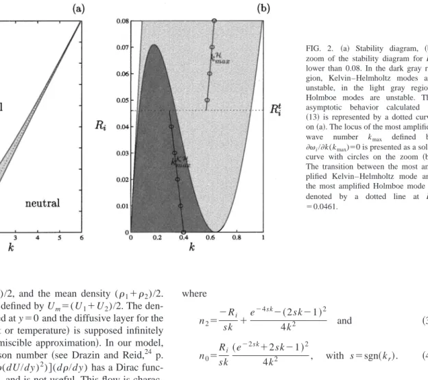
FIG. 2. 共a兲 Stability diagram, 共b兲 zoom of the stability diagram for Ri

lower than 0.08. In the dark gray re-gion, Kelvin–Helmholtz modes are unstable, in the light gray region, Holmboe modes are unstable. The asymptotic behavior calculated in

共13兲 is represented by a dotted curve

on共a兲. The locus of the most amplified wave number kmax defined by

⳵␻i/⳵k(kmax)⫽0 is presented as a solid curve with circles on the zoom 共b兲. The transition between the most am-plified Kelvin–Helmholtz mode and the most amplified Holmboe mode is denoted by a dotted line at Ri t

⫽0.0461.

2587

Phys. Fluids, Vol. 14, No. 8, August 2002 Spatial Holmboe instability

the density interface is displaced with respect to the velocity interface and by Smyth and Peltier14for a hyperbolic tangent velocity profile. We have plotted on Fig. 2共a兲 the stability diagram derived from共2兲. Without stratification, Ri⫽0, there

is a unique unstable mode studied by Rayleigh28 stationary with respect to the mean flow. When the Richardson number increases, the structure is more complex. To get a better un-derstanding of the unstable modes which exist, we discuss the sign of⌬. When ⌬⬎0 and n2⬎0 then we obtain from 共5兲

two unstable, stationary modes. The most amplified one is the continuation of the mode found by Rayleigh,28 the sec-ond one is generated by stratification. These instabilities, which we call following Smyth and Peltier14 Kelvin– Helmholtz waves, are stationary with respect to the mean flow and, correspond to the dark gray region on Fig. 2共b兲. When ⌬⬍0, the unstable modes have intrinsic frequencies with a nonzero real part. Moreover, since under the Bouss-inesq approximation, the basic flow is invariant under the following reflections, x→⫺x and y→⫺y, if ␻(k) is a so-lution then ␻(⫺k) is also a solution and as a consequence

⫺␻¯ (k¯ ) is a solution 共in the temporal case k is real兲. Thus when a mode propagating downstream is amplified, a sym-metric mode propagating upstream is also unstable with the same growth rate. These propagating unstable modes will be called Holmboe waves. They exist in the light gray region on Fig. 2共b兲. When the Richardson number increases, two un-stable Holmboe regions develop at low and high wave num-bers. For Ri⫽0.07, the Kelvin–Helmholtz region disappears

and the two Holmboe regions merge. For Rilarger than 0.07,

the Holmboe region moves to larger k but never vanishes

关Fig. 2共a兲兴.

For further references, we illustrate the structure of the modes when Ri⬍0.07, we consider the case of Ri⫽0.04. We

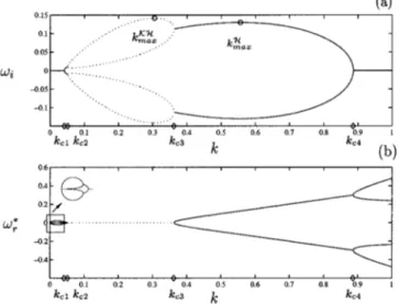
plot on Fig. 3 the growth rate␻i and the intrinsic frequency

␻r*as a function of the wave number k. Close to k⫽0, four

neutral waves exist, two propagating to the right 共␻*⬎0兲, two to the left共␻*⬍0兲. When k⫽kc1, the waves merge two

by two and give rise to two unstable Holmboe modes

共propa-gating to the right and to the left with ␻_i⬎0兲. When k

⫽kc2, the phase speeds of the two Holmboe modes vanish

and two stationary unstable Kelvin–Helmholtz modes ap-pear, the most amplified being the continuation of the homo-geneous mode found by Rayleigh,28the less amplified being generated by the stratification 关dotted curves on Figs. 3共a兲 and 3共b兲兴. At k⫽kc3, the sequence reverses: the growth rates

of the two Kelvin–Helmholtz modes become equal and the character of the instability changes from stationary to oscil-latory. These new Holmboe modes have the same growth rate but propagate in opposite directions with respect to the mean flow 关Fig. 3共b兲兴. For k⫽kc4, the growth rate of the

Holmboe modes vanishes and four neutral waves appear. On Fig. 3共a兲, the temporal growth rate presents two relative maxima k_maxKH and k_maxH associated respectively to Kelvin– Helmholtz and Holmboe modes. For Ri⫽0.04, the Kelvin–

Helmholtz mode is the most unstable 共see Fig. 3兲. On Fig. 2共b兲, we have plotted the locus of the most unstable wave number as a curve with circles. For R_it⫽0.0461, the most amplified mode switches over from Kelvin–Helmholtz-type to Holmboe type.

IV. ABSOLUTE AND CONVECTIVE INSTABILITIES

As described in the Introduction in all the laboratory or field situations where the stratified shear flow may be as-sumed stationary in a particular frame, one should look for the appearance of self-sustained oscillations associated with the absolute nature of the instability in a portion of that flow.19These so-called global modes arise from the building up of energy fluctuation due to the temporal amplification of a wave that does not propagate共of zero group velocity in the frame where the mean flow is stationary兲. This idea, first developed in plasma physics 共Briggs,29 Bers30兲, is fully dis-cussed in Huerre and Monkewitz19 and leads to a discrimi-nation between convective or absolute instability. According to a well established criterion the absolute/convective insta-bility distinction is obtained by studying the behavior of spa-tial branches共k⫽kr⫹ikicomplex,␻real兲, or more generally

spatio-temporal branches 共k and ␻⫽␻r⫹i␻i complex; ␻r

varying and␻ibeing constant兲. The transition occurs when a

saddle point of the dispersion relation (k0,␻0) crosses the␻i

axis

D共k0,␻0;Ri,a兲⫽0, 共7兲

⳵kD共k0,␻0;Ri,a兲⫽0, 共8兲

⳵␻D共k0,␻0;Ri,a兲⫽0, 共9兲

with k₀ the absolute wave number and␻₀ the absolute fre-quency. For shear flow, the dispersion relation contains the non analytic function sgn(k) 关see Eqs. 共3兲–共5兲兴. The sign function arises from the constraint that perturbations should decay at y⫽⫾⬁. In order to obtain an analytic function for the dispersion relation 共5兲 in k, we restrict the study to kr ⬎0 as in Huerre and Monkewitz,31 _{invoking the symmetry}

␻(k)⫽⫺␻¯ (⫺k¯) and then s⫽sgn(kr)⫽1 in 共2兲–共4兲. If the

imaginary part of␻0, Im(␻0), is positive, the flow is

abso-lutely unstable. Conversely ifIm(␻0) is negative, the flow is

convectively unstable. Conditions 共7兲–共9兲 are not explicit FIG. 3. 共a兲 Temporal growth rate␻i and共b兲 intrinsic frequency␻r*⫽␻r

⫺ak with respect to the real wave number k for Ri⫽0.04. The dotted curve

shows the Kelvin–Helmholtz modes.

enough, and the saddle point to be considered must also sat-isfy a pinching condition of two spatio-temporal branches k⫾(␻) arising, respectively from the upper and the lower halves of the (kr,ki) plane19 共i.e., ki⬎0 and ki⬍0兲. In the

convective case, the superscript ⫹ or ⫺ gives the direction of propagation of the wave in the laboratory frame 共see Huerre and Monkewitz19for details兲.

We used the Optimization toolbox of MATLAB to solve the systems 共7兲–共9兲. Once (k0,␻0) was found, we

system-atically checked the pinching condition. The domains of ab-solute and convective instability are plotted on Fig. 4 in the (a,Ri) plane. Due to the symmetry of the problem, when a is

changed to ⫺a, y is changed to ⫺y, so we focus in the following discussion on a⬎0.

As could be seen on Figs. 4共a兲 and 4共b兲, when both streams move in the same direction (a⬎1), the flow is con-vectively unstable whatever the value of the Richardson number, i.e., no matter how strong the stratification. When the streams propagate in opposite directions (a⬍1), two cases must be distinguished. When both Kelvin–Helmholtz and Holmboe modes are unstable, for Ri⬍0.07, the flow is

absolutely unstable in the whole domain 关0,1关. Whereas, when only Holmboe modes are unstable, for Ri⬎0.07, the

flow is convectively unstable for mean advection smaller than a threshold value ac(Ri), and absolutely unstable in a

range, ]ac(Ri),1关. The structure of Fig. 4, may be easily

understood referring to the impulse response of the flow

共Fig. 5兲. Since the impulse response is invariant under

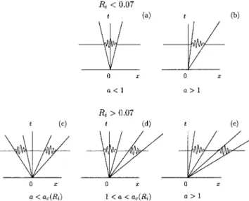
Gal-lilean transformation, its shape is the same whatever the value of the advection parameter. Therefore, a change in the mean advection parameter a corresponds to a change of Gal-lilean frame. For Ri⬍0.07, the absolute–convective

transi-tion is associated with the classical picture: a single ampli-fied domain for the impulse response. However, the structure of the wave packet is complicated. It is a result of an hybrid-ization of the Kelvin–Helmholtz and Holmboe modes. The edges of the impulse wave packet move at velocity a⫺1 and a⫹1. For a smaller than unity, the flow is absolutely

un-stable关Fig. 5共a兲兴. For a larger than unity the flow is convec-tively unstable 关Fig. 5共b兲兴. For Ri⬎0.07, two Holmboe

modes destabilize the flow and the impulse response pos-sesses two amplified regions with edges moving respectively at a⫺1 and a⫺ac(Ri) and at a⫹ac(Ri) and a⫹1. The case

of the destabilization by two traveling waves was already investigated at the onset of convection in binary fluids.23 In contrast with binary convection which endows the reflec-tional symmetry (x↔⫺x) 共see Huerre et al.,19 Kolodner, Surko, and Williams23兲, the free mean advection parameter, a, of the present model flow, breaks the reflectional symme-try and makes the discussion richer. Three possible configu-rations may be encountered depending on the value of a positive 共the case a⬍0 being symmetric兲. For a⬍ac(Ri) 关Fig. 5共c兲兴 the wave packets move away from the source to

the left and the other to the right and the flow is, therefore, convectively unstable 关white region on the left of the Fig. 4共a兲兴. When a_c(R_i)⬍a⬍1 关light gray region in Fig. 4共a兲兴 the left moving wave packet is now making the flow absolutely unstable since it is exponentially growing at the impulse lo-cation关Fig. 5共d兲兴. The absolute instability is, therefore, trig-gered by the Holmboe wave associated with the lower layer. When a⬎1, both waves packets propagate to the right 关Fig. 5共e兲兴, and the flow is again convectively unstable 关right white region in Fig. 4共a兲兴.

Two characteristics in the flow behavior visible on Fig. 4 should be pointed out. First, a⫽1 defines a transition from absolute to convective instability for all Ri. For Ri⫽0, this

result was obtained by Balsa32and by Bechert.33In Sec. VI, a large k asymptotic expansion will explain the particular significance of the a⫽1 value. Second, the transition at Ri ⫽0.07 from a single wave packet to a double wave packet is

abrupt as the Kelvin–Helmholtz modes become stable. V. SPATIAL INSTABILITY

Spatial waves have been much debated due to their un-bounded behavior at 兩x兩→⬁ 共Drazin and Reid,24 pp. 147–

FIG. 4.共a兲 In light gray, absolute instability, A, in white convective insta-bility, C, in the (a,Ri) plane. The asymptotic behavior calculated in共24兲 is

represented by a dotted curve; 共b兲 zoom of the absolute and convective domains for Ri⬍0.2.

FIG. 5. Sketch of the impulse response in the (x,t) plane. For Ri⬍0.07 a

single wave packet, 共a兲 absolutely unstable for a⬍1 and 共b兲 convectively unstable for a⬎1. For Ri⬎0.07 behavior of the two Holmboe wave packets

for a positive varying as indicated on the figure.

2589

Phys. Fluids, Vol. 14, No. 8, August 2002 Spatial Holmboe instability

153兲. However when the flow is convectively unstable, they appropriately describe the asymptotic response as t→⬁ to a spatially localized harmonic source turned on at the origin of time 共see Chomaz34兲. In this case, initial transients, due to the switching on of the harmonic forcing, are advected away from the forcing excitation. The spatially amplified waves radiated from the source are left behind this transient wave packet and may be interpreted in terms of spatial causality. In absolutely unstable flows, transients exponentially growing in time do not propagate away and overwhelm the forcing response. As for temporal theory, the structure of spatial in-stability branches will differ for R_i larger or smaller than

0.07. The case R_i⬍0.07 will be more complex since Kelvin– Helmholtz and Holmboe modes that are well separated in the temporal theory will mix and following Pawlak and Armi,22 we will name the domain R_i⬍0.07, the hybrid region. A. Hybrid region

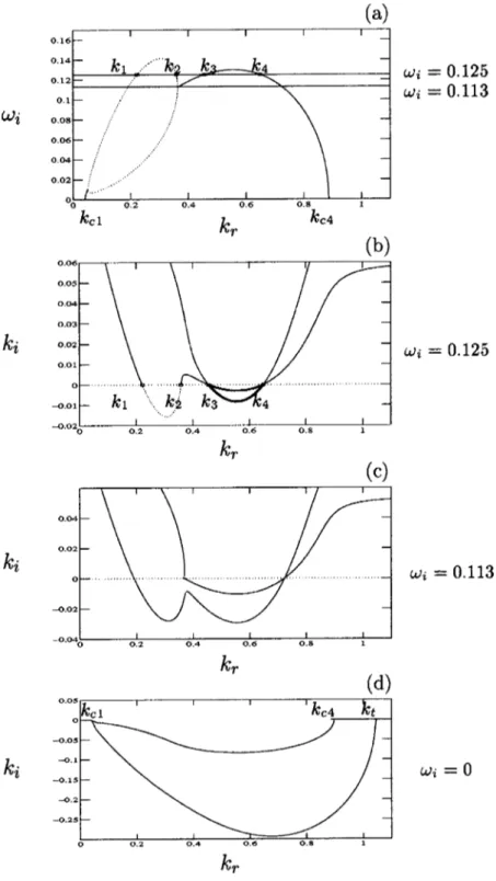
For R_i⬍0.07, and in the particular case of wedge flows (a⫽1), Pawlak and Armi22 found numerically, using the Taylor–Goldstein equation, two propagating spatially grow-ing modes. They called them hybrid modes since in the spatial case no straightforward criteria discriminates between FIG. 6. In dotted curve, Kelvin–Helmholtz branches. In solid curve Holmboe branches共a兲 temporal growth rate

␻ifunction of the wave number krfor Ri⫽0.04;

spatio-temporal branches for Ri⫽0.04 and a⫽1.1␻r varies

between 0 and 1.5 by small increments 共b兲 for ␻i

⫽0.125, 共c兲 pinching of amplified branches and ex-change of branches for␻i⫽0.113, and 共d兲 hybrid

spa-tial branches␻i⫽0.

Kelvin–Helmholtz and Holmboe modes. In order to gain some insight into these hybrid modes, and to illustrate the existence of saddle points in the dispersion relation that do not lead to an absolute–convective transition, we consider the deformations of the spatio-temporal branches as the ␻ contour is lowered from high values of ␻i toward␻i⫽0, in

the case Ri⬍0.07 and a⬎1. We plot on Figs. 6共b兲–6共d兲, only

the downstream amplified branches. All the branches are ob-tained by solving numerically the dispersion relation共2兲 us-ing MATLAB Optimization routines for a particular set of fixed parameters␻_i, R_i, and a and with␻_r varying. These branches are parametrized by ␻_r which varies by small in-crements共see Loiseleux, Chomaz, and Huerre for details35兲. Figure 6共a兲 reproduces Fig. 3共a兲 and presents the temporal growth rate for R_i⫽0.04 and a⫽1.1. When␻_i⫽0.125, the wave numbers k1, k2, k3, and k4 belonging to the unstable

temporal branches关Fig. 6共a兲兴, also belong to the downstream spatio-temporal branches for␻i⫽0.125 plotted on Fig. 6共b兲.

We note two downstream amplified branches on Fig. 6共b兲. For the first branch, the two unstable parts in the dotted curve between k1and k2 and in the heavy curve between k3

and k4, may be associated respectively to Kelvin–Helmholtz

and Holmboe modes. The second downstream unstable branch is unstable between k3 and k4, which corresponds to

the most spatially amplified Holmboe branch. The least am-plified Kelvin–Helmholtz branch is associated with a damped spatio-temporal branch 共i.e., ki⬎0兲 since ␻i

⫽0.125 is larger than its maximum growth rate (␻i

⬃0.113). While lowering the ␻i contours, we may follow

the deformations of those branches. In this process, a saddle point is encountered for ␻i slightly larger than 0.113, but it

does not involve an interaction between two branches arising from different part of the kiplane. This saddle point does not

contribute to the impulse response.19The branches plotted on Fig. 6共c兲 are a result of this interaction. The effect of this saddle point has been to ‘‘hybridize’’ the two Kelvin– Helmholtz modes with the two Holmboe modes, but all four modes keep propagating information downstream. Finally, on Fig. 6共d兲, we obtain the two downstream amplified spatial branches共␻real兲. Another saddle point which is once again not a pinch point is encountered for ␻i⬃0.0099 when the

small wave number Holmboe modes destabilize 关k

苸关kc1,kc2兴 Fig. 3共b兲兴. This continuous switching of

branches justifies the terminology hybrid mode.

The structure of the hybrid branch near k⫽ktplotted on

Fig. 6共d兲 is surprising in the sense that a neutral mode 共i.e.,␻ and k real兲 is a spatio-temporal wave that belongs both to the temporal and to the spatial branches as is the case for k

⫽kc1 and k⫽kc4. Therefore, it should appear both as a

crossing of the temporal branch with the ␻i⫽0 axis 关Fig.

6共a兲兴 and as a crossing of the spatial branch with the ki⫽0

axis 关Fig. 6共d兲兴. But the most amplified branch seems to cross at k⫽ktand to have no temporal counterpart. When␻i

is small but nonzero the spatio-temporal branch crosses the ki⫽0 axis close to k⫽kc4 as it should, but prior to this

crossing it makes a large turn about close to kt and then

reaches kc4 parallel to the ki⫽0 axis 关continuous curve on

Fig. 7共a兲兴. The smaller␻i, the closer this final portion of the

spatio-temporal branch to the ki axis. Finally when ␻i

van-ishes, the branch becomes singular 关dotted curve on Fig. 7共a兲兴 and seems to cross at k⫽kt. Clearly, the limit␻i⫽0 is

singular since the most unstable spatial branch collapses on the ki⫽0 axis at k⫽kt关Fig. 7共a兲兴. Therefore, k⫽ktis only a

pseudo-intersection of the most unstable branch with the ki ⫽0 axis since k⫽ktis never reached. The dispersion relation 共5兲 exhibits a square root behavior at the neutral

wavenum-ber, kc4 共see also Fig. 3兲. Therefore, a branch cut lies from

kc4 to infinity共Fig. 7兲 in the k plane. This singular behavior

is reponsible for the a⫽1 transition. When a decreases from a⫽1.1 to a⫽1.000 001 关Fig. 7共b兲兴, the pseudo-intersection, kt, of the hybrid branch with the branch cut moves to large

value. At a⫽1, kt tends to infinity, and the pinching of the

real axis occurs at ⫹⬁ and not as usual at a finite saddle point. In fact, an infinity of spatial branches, shown on Fig. FIG. 7. 共a兲 Comparison between the most amplified spatio-temporal branches in solid curve at small values of ␻i and between the spatial

branches ␻i⫽0 in dotted curve for two values of a, a⫽1.01 and a

⫽1.000 001. 共b兲 Behavior of the most amplified hybrid spatial branch, Fig. 6共d兲, for Ri⫽0.04 and for a⫽1.1, a⫽1.01 and a⫽1.0001, and a

⫽1.000001; kc4is the neutral wave number defined on Fig. 3.

FIG. 8. 共a兲 Simultanously pinching of several branches at a⫽1 and Ri

⫽0. 共b兲 Bechert Christmas tree 共Ref. 33兲 for a⫽1 and Ri⫽0.

2591

Phys. Fluids, Vol. 14, No. 8, August 2002 Spatial Holmboe instability

8共a兲, go through a similar transition at the same time 关Fig. 8共a兲兴. Plotted in the (k_i,␻_r) plane for the particular case R_i

⫽0, these branches evoke an upside down Christmas tree in

Bechert’s imagination33 关Fig. 8共b兲兴. This singularity leads to an essential singularity of the dispersion relation. In Sec. VI, we will see that this behavior persists for all values of the Richardson number.

B. Holmboe spatial modes

When Ri⬎0.07, the Kelvin–Helmholtz mode is

stabi-lized and two counterpropagating Holmboe waves destabi-lize the flow. As a result, the instability is convective in two distinct domains, 0⬍a⬍ac(Ri) and a⬎1 as shown on Fig.

4. The structure of the spatial branches belonging to each of the convectively unstable domains are shown on Fig. 9.

When the mean advection a is smaller than a_c(R_i), the response to an impulse consists of two wave packets travel-ing in opposite directions 关Fig. 5共c兲兴. The mode traveling with the negative group velocity is amplified upstream and the corresponding amplified spatial branch is characterized by ki⬎0. It is represented on Fig. 9共a兲 by a solid curve. In

contrast the other Holmboe mode travels downstream and the corresponding amplified spatial branch represented by a dotted curve on Fig. 9共a兲 is such that ki⬍0. On Fig. 9共c兲 the

spatial growth rates are represented as a function of the fre-quency. Waves moving upstream are represented by negative ␻rvalues since kr is assumed positive by convention.

When the mean advection a is larger than unity, the flow is convectively unstable and the impulse response is associ-ated with two wave packets, both traveling downstream关Fig. 5共e兲兴. The mode traveling with the smaller group velocity is the most spatially amplified, and is represented by a solid curve on Figs. 9共b兲 and 9共d兲. This contrasts with the temporal theory for which both Holmboe modes have the same ampli-fication rates. Qualitatively, these results may be understood using the Gaster transformation,36 which gives, in the limit of small amplification rates, the link between the spatial and temporal amplification rates at the same real wave number kr

␻i

ki ⬃⳵␻r

⳵kr共kr兲⬃⫺vg

. 共10兲

However, as discussed in a later section, much care must be taken using Eq.共10兲 since the Gaster transformation is valid only under certain assumptions.36 Figure 9共d兲 presents the spatial growth rate as a function of the wave frequency␻r.

Since both waves are propagating downstream, ␻r is

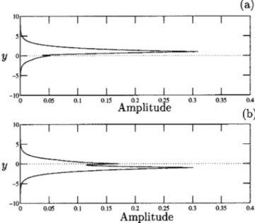
posi-tive, but the range of frequencies associated with the slower moving wave is smaller. For the slower moving wave共higher growth rate and smaller frequency兲, the eigenfunction is more intense in the slower moving layer 关Fig. 10共b兲兴. Con-versely, the other spatially unstable branch, with a smaller spatial growth rate and a larger frequency is localized in the FIG. 9. Amplified spatial Holmboe branches for Ri

⫽0.5. In solid curve Holmboe branch associated with the lower frequency, in dotted curve Holmboe mode associated with the greater frequency;共a兲 kifunction of

the wave number krfor a⫽0.1 and 共b兲 for a⫽1.2; 共c兲

ki function of the frequency␻r for a⫽0.1, 共d兲 for a

⫽1.2.

FIG. 10. Amplitude of the eigenfunction for Ri⫽0.5, a⫽1.2 associated with

each most amplified wave number on each Holmboe branch关see Fig. 9共b兲兴. On共a兲, eigenfunction associated with the Holmboe mode traveling with the faster layer共i.e., the upper layer here兲 共b兲 eigenfunction of the most ampli-fied wave number traveling with the lower layer.

fast moving stream 关Fig. 10共a兲兴. The difference in spatial growth rates suggests that the Holmboe mode concentrated in the slower layer关Fig. 10共b兲兴 may dominate in experiments when broadband forcing is applied at the inlet. However, since Holmboe modes are unstable over different frequency bands as shown on Figs. 9共c兲 and 9共d兲, an appropriate forc-ing at the inlet may select experimentally one or the other mode.

VI. ASYMPTOTIC RESULTS

In the inviscid approximation, the configuration of Fig. 1 is unstable to wavelength that goes to zero (k→⬁) when the strength of the stratification increases, i.e., when Ri→⬁ 关Fig.

2共a兲兴. In this section, we carry out an asymptotic expansion of the dispersion relation in the limit k_r→⬁. We will con-sider first the case R_i→⬁ and in a second part R_ifinite. This analysis explains on physical grounds the convective– absolute transitions computed numerically.

Neglecting all terms of order less than exp(⫺3k_r), the complex frequency共5兲 becomes with k real or complex but kr large ␻⯝ak⫾ k

冑

2

冑

Ri k ⫹ 共2k⫺1兲2 4k2 ⫾

冑

⌬asymp⫹o共e ⫺3kr兲. 共11兲

In the above expression,⌬asympis the asymptotic value of共6兲

defined by ⌬asymp⯝

冉

Ri k⫺ 共2k⫺1兲2 4k2

冊

2 ⫺2Ri共2k⫺1兲ke⫺2k k4 ⫹o共e ⫺3kr兲. 共12兲 A. Asymptotics at largeRi

Temporally amplified modes共k real兲 are obtained when

⌬asymp共12兲 is negative. For large k away from the unstable

band of wave numbers,⌬asympisO(1/k4). However, for the

particular wave number kmsuch that

Ri⫽

共2km⫺1兲2

4k_m , 共13兲

the function⌬_asympis of order e⫺2km_/k

m. For this particular

value of k_m, we obtain ⌬_asymp minimal and negative. The expression 共13兲 has been already derived by Caulfield37 in the form R_i⫽k_m⫺1. The most amplified wave number k_mis represented by a dotted curve on Fig. 2共a兲. Moreover, as can be seen on Fig. 2共a兲, the stronger the stratification, the nar-rower the band of temporally unstable wave numbers. There-fore, in order to obtain the asymptotic expansion of the dis-persion relation, we let Ri goes to infinity and we seek the

wave numbers close to kmfor which, the two terms of

right-hand side of 共12兲 have the same order and ⌬asymp negative.

Therefore, we write

k⫽k_m⫹⑀k

⬘

, 共14兲

with km given by 共13兲 k

⬘

real or complex and the gauge ⑀

determined by the dominant balance

⑀⫽

冑

k_me⫺km_. 共15兲

The dispersion relation 共11兲 may be rewritten at order ⑀as followed with s1⫽⫾1 and s2⫽⫾1 independent

␻⫽akm⫹⑀ak

⬘

⫹s1km⫺ s1 2 ⫹⑀s1k

⬘

冉

3 4⫺ 1 8km

冊

⫹⑀s2 2km⫹1 8k_m

冑

k

⬘

2_⫺8km共2km⫺1兲 共2km⫹1兲 2 . 共16兲

The unstable temporal wave numbers共k

⬘

real兲 are obtained for k

⬘

2⫺8km(2km⫺1)/(2km⫹1)2 negative, which specifies

the band of unstable wave numbers k⫽km⫹⑀k

⬘

with k

⬘

苸

冋

⫺

冑

8km共2km⫹1兲 2km⫹1 ,

冑

8km共2km⫹1兲 2km⫹1

册

, 共17兲

then at leading order in⑀the frequency of an unstable wave number k 共17兲 is given by ␻r⫽akm⫹⑀ak

⬘

⫹s1km⫺ s1 2 ⫹⑀s1k

⬘

冉

3 4⫺ 1 8k_m

冊

, 共18兲 with a growth rate

␻i⫽⑀ 2km⫹1 8k_m

冑

8km共2km⫺1兲 共2km⫹1兲 2 ⫺k

⬘

2. 共19兲

The complex frequencies (␻r⫹i␻i) of the temporally

ampli-fied Holmboe modes associated with the most unstable wave number kmare obtained letting k

⬘

⫽0 in 共18兲 and 共19兲

␻m⫾⫽

再

akm⫾

冉

km⫺ 1 2

冊冎

⫹i⑀

冑

2k_m⫺1

冑

8km , 共20兲

the associated group velocity is obtained calculating ⳵␻/⳵k for ␻given by共16兲 and evaluated at k

⬘

⫽0

vG共km兲⫽ ⳵␻ ⳵k共km兲⫽ 1 ⑀ ⳵␻ ⳵k

⬘

共0兲 ⫽a⫾

冉

3₄⫺_8k1 m

冊

→a⫾3₄. 共21兲 The results共17兲–共21兲 match quantitatively well with numeri-cal numeri-calculations.

The absolute unstable branch may be computed using the dispersion relation 共16兲 derived for k

⬘

real or complex. Imposing⳵␻/⳵k⫽0 with␻and k⫽km⫹⑀k

⬘

linked by共16兲,

give the absolute frequency␻0 and wave number k0

⬘

k₀

⬘

⫽

冉

a⫹s₁

冉

3 4⫺ 1 8km

冊冊

冑

8km共2km⫺1兲 共2km⫹1兲

冑

共a⫹s1兲

冉

a⫹s1

冉

1 2⫹ 1 4k_m

冊冊

, 共22兲 2593

Phys. Fluids, Vol. 14, No. 8, August 2002 Spatial Holmboe instability

␻0⫽akm⫺s1

冉

km⫺ 1 2

冊

⫹⑀k0

⬘

⫻

冋

共a⫹s1兲

冉

a⫹s1

冉

1 2⫺ 1 4km

冊冊

a⫹s1

冉

3 4⫺ 1 8k_m

冊

册

. 共23兲

The absolute–convective transition corresponds to the imagi-nary part of␻0equals to zero, which yields according to共13兲

and with s₁⫽⫾1 a_c共R_i兲⫽⫾

冉

1 2⫺ 1 4km

冊

⫽⫾

冉

1₂⫺ 2 1⫹Ri⫹

冑

共1⫹Ri兲2⫺1

冊

共24兲 and a⫽⫾1. 共25兲

The transition a⫽1 共25兲 obtained at large Ri, corresponds

exactly with the numerically computed threshold 关Fig. 共4兲兴. The second transition ac(Ri) given on Eq.共24兲 is represented

by a dotted line on Fig. 4共a兲, the asymptotic calculus matches remarkably well the numerical calculation. At the limit km

→⬁, ac tends to 1/2.

Moreover, when the advection parameter a approaches one of the two thresholds共24兲 or 共25兲, 兩k₀

⬘

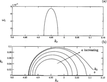
兩 tends to infinity, this suggests that the spatial growth rate is greater than the temporal one near the threshold. Numerically, we compare near the first threshold ac(Ri) on Fig. 共11兲 the spatial and

temporal amplification rates of the Holmboe mode amplified upstream (ki⬍0), for Ri⫽4. We note that the band of

tem-poral unstable wave numbers, which matches exactly with

共17兲, is smaller than in the spatial case for the advection

parameter approaching the transition a_c⫽0.4368. The

differ-ence of growth rates in temporal and spatial case near the thresholds enhances the failure of the Gaster transformation

关Eq. 共10兲兴 in those cases 共see Sec. VII兲.

B. Asymptotics at finiteR_i

The dispersion relation displays two amplified and two damped solutions. The branch leading to the pinching is the Holmboe mode traveling with the smaller phase velocity

关Fig. 5共d兲兴. Choosing the principal square root such that Z1/2

maps the complex Z-plane cut along the negative real axis onto the half space Re(Z1/2)⬎0, the amplified spatial branch

downstream is recovered solving ␻⯝ak⫺ k

冑

2

冑

Ri k ⫹ 共2k⫺1兲2 4k2 ⫹

冑

⌬asymp ⫹o共e⫺3kr兲. 共26兲

The threshold a⫽1 共25兲 is independent on Ri. Moreover as

shown in the hybrid region in Fig. 7, when the advection parameter a tends to unity, the absolute wave number k0

pinches at infinity for any value of R_i. We propose to cap-ture this behavior assuming R_iof order unity and k complex but k_r large. Under this assumption, the square term in

⌬asympgiven in 共12兲 is always dominant with respect to the

second term. Neglecting the terms of order equal or less than e⫺2k/k2, we obtain ⌬asymp⬃

冉

R_i k⫺ 共2k⫺1兲2 4k2

冊

2 ⫹O

冉

e⫺2k_k

冊

. 共27兲

For k complex but kr large the dispersion relation becomes

␻⫽ak⫺2k₂⫺1. 共28兲

The absolute frequency and wave number are obtained solv-ing ⳵␻/⳵k⫽0

⳵␻

⳵k⫽a⫺1⫽0. 共29兲

For a⫽1, the absolute wave number tends to ␻0⫽1/2

and the absolute wave number k0 is not determined. The

value of this absolute frequency is retrieved numerically, in this paper we have only represented the classical Bechert Chritmas tree,33 共Fig. 8兲 共that means for Ri⫽0兲 included in

this analysis.

As a conclusion of the asymptotic studies, the absolutely unstable domain goes to a⫽1/2 to a⫽1 as Ri goes to

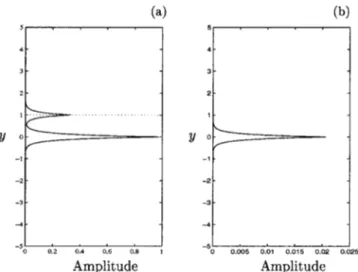
infin-ity. At the trailing edge the first threshold 共24兲 tends to 1/2, the group velocity of a pure gravity wave with a phase ve-locity equals to 1. Indeed the computed eigenfunction corre-sponding to this mode关given in Fig. 12共b兲兴 has a large am-plitude only around the density interface and indeed, corresponds to a gravity wave marginally destabilized by the interaction with the density interface. At a⫽3/4, the most amplified modes differ from gravity waves, the associated eigenmode being intense both at y⫽1 and y⫽0 关Fig. 12共a兲兴. At the leading edge of the wave packet, a⫽1, only the layer FIG. 11. Comparison between共a兲 the temporal amplification rate␻iand共b兲

the spatial amplification rate kifor the Holmboe branch traveling with the

lower layer for Ri⫽4, and several values of the advection parameter a

⫽0.42, a⫽0.43, a⫽0.435, and a⫽0.438 where the pinching k0occurs.

at y⫽⫺1 is active, and the mode is insensitive to Ri, but

since the pinching occurs at infinity no eigenmode may be exhibited.

VII. DISCUSSION AND CONCLUSION

For Ri⫽4 and for different values of the advection

pa-rameter a from 0.2 to 1.5, we have plotted on Fig. 13 共resp. Fig. 14兲, the spatial amplification rates ki of the right-going

Holmboe mode 共resp. left-going mode兲 as a function of the intrinsic frequency␻_r* obtained solving numerically the dis-persion relation 共2兲. The right-going and the left-going Holmboe modes are represented by a solid curve on Figs. 13 and 14. We will compare those branches with predictions of

the spatial amplification rates obtained transforming the tem-poral growth rate using Gaster transformation36 recalled here. For a given real wave number k˜r, the temporal analysis

leads to␻⫽␻r(k˜r)⫹i␻i(k˜r) complex solution of the

disper-sion relation共2兲. We seek for this particular wave number the value of the spatial amplification rate k˜i such that ␻(k˜r ⫹ik˜i) denoted ␻S is real. For small amplification rates, we

make a Taylor expansion of ␻S for k˜i small. If we suppose

that ␻ is an analytical function of k, the Cauchy–Riemann relation holds and the Taylor expansion becomes

␻S⫽␻r共k˜r兲⫹i␻i共k˜r兲⫺k˜i ⳵␻i ⳵kr 共k˜ r兲⫹ik˜i ⳵␻r ⳵kr 共k˜ r兲⫹O共k˜i 2_兲. 共30兲

We conclude that for k˜i(⳵␻i/⳵kr)(k˜r) small, the frequency

associated with k˜r is the same in the temporal case (k˜i⫽0)

and in the spatial case 关Im(␻s)⫽0兴

␻S⬃␻r共k˜r兲. 共31兲

Moreover, since spatial mode corresponds to find k˜isuch

that ␻s is real, we obtain, except if the group velocity

⳵␻r/⳵kr(k˜r) vanishes k ˜ i⫽⫺ ␻i共k˜r兲 ⳵␻r ⳵k_r 共k˜r兲 . 共32兲

For R_i⫽4, the temporal amplification rate ␻_ihas been plot-ted on Fig. 11共a兲. The spatial amplification rate obtained from Gaster transformation k˜i is computed by 共32兲 for each

value of the wave number. For this value, the frequency␻S

associated to the spatial mode is obtained from the temporal theory 共31兲. For a varying from 0.2 to 1.5, we plot as a dotted curve the spatial amplification rates thus obtained as a function of␻S for the right-going mode共Fig. 13兲 and for the

left-going mode 共Fig. 14兲.

For the right-going Holmboe mode represented on Fig. 13, the dotted branches obtained from共31兲 and 共32兲 fit very FIG. 12. 共a兲 Amplitude of the eigenfunction associated with␻m⫹共20兲 and

with the most amplified wave number kmfor Ri⫽8. 共b兲 Amplitude of the

eigenfunction associated with the wave number k0 and with the absolute

frequency␻0关see on Fig. 12共b兲兴 for Ri⫽4 and a⫽0.438, that means for the

first convective–absolute transition.

FIG. 13. Spatial growth rate of the right-going Holmboe wave versus the intrinsic frequency ␻r*, for Ri⫽4 and different values of the advection

parameter a, a⫽1.5, a⫽1.01, a⫽0.43, and a⫽0.2. In solid curve, Holmboe branches obtained by solving the dispersion relation, in dotted curve by following the Gaster transformation共10兲.

FIG. 14. Spatial growth rate for the left-going Holmboe wave versus the intrinsic frequency ␻r*, for Ri⫽4 and different values of the advection

parameter a, a⫽1.5, a⫽1.01, a⫽0.43, and a⫽0.2. In solid curve, Holmboe branches obtained by solving the dispersion relation, in dotted curve by following the Gaster transformation共10兲.

2595

Phys. Fluids, Vol. 14, No. 8, August 2002 Spatial Holmboe instability

well the spatial branches obtained numerically 共in solid curve兲. For the left-going Holmboe mode far from the convective–absolute instability thresholds a⫽0.438 and a

⫽1, the Gaster transformation 共32兲 gives a good prediction

of the spatial amplification rate. Near the two thresholds, a

⫽0.43 and a⫽1.01, the solid and dotted curves are very

different. The group velocities are very small, the spatial growth rate is large and the Taylor expansion 共30兲 is no longer valid since terms of order k_i2 can no longer be ne-glected. Close to a⫽1, the failure is also imputable to the nonanalyticity of the dispersion relation near the branch cut where the ‘‘pinching at infinity’’ occurs. Cauchy–Riemann relations do not hold, and so the expansion given in共30兲 is no longer valid. We conclude that, except close to the absolute–convective thresholds, the Gaster transformation predicts remarkably well the spatial instability.

In Exchange flows, the two layers flow in opposite di-rections. Such flows are characterized in our model共Fig. 1兲 by a mean advection a between 0 and 1共by convention a is positive兲. When the Richardson number is lower than 0.07, exchange flows are absolutely unstable in the whole range

关0,1关 共Fig. 4兲, and are able to exhibit self-sustained

oscilla-tions. In contrast when Riis larger than 0.07, exchange flows

are absolutely unstable for mean advection larger than ac(Ri) and once again self-sustained oscillations may occur.

For a smaller than ac(Ri), the flow is convectively unstable,

but since both upstream and downstream propagating spatial branches are unstable, a self-sustained resonance may be eas-ily triggered by reflective boundary conditions and the dy-namics of exchange flow deserve further analysis.

Wedge flows are a particular case of exchange flows, with one layer arrested. In our model 共Fig. 1兲, they corre-spond to a⫽1. These flows are marginal since the transition from absolute to convective instability occurs at a⫽1 for all values of R_i. This result is not an artifact induced by the singularity of the broken line velocity profile used to model the flow. Indeed, Balsa38 has shown numerically for R_i⫽0, that a smoothing of the velocity profile imposed at the edges of the shear layer near y⫽⫾1 共Fig. 1兲 does not modify this absolute–convective transition. Of course, strong changes in the velocity profile used to model the shear are known to modify the threshold. As an example, in the case of a homo-geneous hyperbolic tangent velocity profile, the theoretical study carried out by Huerre and Monkewitz31 for homoge-neous mixing-layers (Ri⫽0) has revealed that the threshold

value is a⫽0.760 instead of a⫽1. This explains why Pawlak and Armi,22investigating linear spatial instability in the case of Boussinesq approximation, for a flow modeled by hyper-bolic tangent velocity and density profiles with different thickness characteristics, found that the instability was con-vective at a⫽0.89. Nevertheless, in their experiments, Paw-lak and Armi22 put forward a very regular regime which consists of a first roll up of the interface as in the homoge-neous case. This first vortex core separates from the vorticity source and a second core develops which pairs with the first one. This mechanism, called ‘‘leapfrog pairing,’’22 persists into fully developed regions and might be the signature of a self-sustained mode 共see Brancher and Chomaz39 for a dis-cussion in the case R_i⫽0兲. Further experiments are needed

to determine whether or not self-sustained oscillations are observed in exchange flows.

In Mixing-layers, the two layers flow in the same direc-tions. Such flows are characterized in our model 共Fig. 1兲 by a mean advection a larger than unity. Whatever the stratifi-cation, unstable mixing-layers are convectively unstable

共Fig. 4兲. Convectively unstable flows are well known to be

extremely sensitive to external forcing. Figures 9共c兲 and 9共d兲 have shown that the two Holmboe modes may be well sepa-rated in frequency for a particular value of the Richardson number. We believe that this frequency selection mechanism may explain the observations of Browand and Wang17 in a stratified channel. They demonstrate that depending on the activation or not to an harmonic forcing on the splitter plate separating the two layers of fluids, one or two traveling waves were observed. At finite amplitude, the two Holmboe waves which form cusps in the upper and the lower layer10 are not always observed experimentally. Koop and Browand,11in their experiment, introduced dye separately in the upper and lower layer. They reported a rolling up of dye, indicating a concentration of vorticity, only in the layer hav-ing the smaller velocity 共the upper one in their experiment兲 and a cusp of the interface only in this layer. This phenom-enon was called ‘‘one-sidedness’’ by Maxworthy and Browand.12 Recently, Zhu and Lawrence,40 in exchange flows apparatus, obtained the experimental evidence of both Holmboe waves 共the two traveling waves兲 and one-sided Holmboe wave共one traveling wave兲. One-sided waves arise from the result of a loss of symmetry of the flow. For Haigh and Lawrence,41there are two ways for the background flow to lose its symmetry: either by displacing the density inter-face with respect to the center of the shear layer or by having horizontal boundaries placed at different distances from the center of the shear layer.41Whereas this is true for temporal theory or numerical experiments in periodic boxes when the symmetry is unbroken, in the spatial theory or in real experi-ments as soon as a is not zero, the symmetry is broken by the inlet condition. The frequency of the Holmboe wave devel-oping in the slower layer is smaller and its spatial growth rate is larger than its symmetric counterpart as shown on Fig. 9. If a white noise is imposed at the inlet then, as in Koop and Browand’s experiments,11the Holmboe mode propagat-ing with the slower stream should dominate the evolution. If the flow is forced by a wave-maker or by an external noise for example at a particular frequency, it seems possible to favor the growth of the other mode since they are unstable to different frequency ranges.

ACKNOWLEDGMENTS

The authors are grateful to G. Pawlak, L. Armi, P. Huerre, Olivier Pouliquen, and Burt Tilley for helpful discus-sions. Special thanks go to L. Tuckerman for her careful reading of the manuscript.

1_{L. Armi and D. M. Farmer, ‘‘The flow of Mediterranean water through the} Strait of Gibraltar,’’ Prog. Oceanogr. 21, 1共1988兲.

2_{G. Pawlak and L. Armi, ‘‘Hydraulics of two-layer arrested wedge flows,’’} J. Hydraul. Res. 35, 603共1997兲.

3_{D. M. Farmer and H. Freeland, ‘‘The physical oceanography of fjords,’’} Prog. Oceanogr. 12, 147共1983兲.

4_{P. Pettre and J. C. Andre, ‘‘Surface-pressure change through Loewe’s} phe-nomena and katabatic flow jumps. Study of two cases in Adelie Land Antartica,’’ J. Atmos. Sci. 48, 557共1991兲.

5

J. E. Simpson, Gravity Currents: In the Environment and the Laboratory

共Ellis Horwood, Chichester, 1987兲.

6_{J. W. Miles, ‘‘On the stability of heterogeneous shear flow,’’ J. Fluid Mech.} 10, 496共1961兲.

7_{L. N. Howard, ‘‘Note on a paper of John W. Miles,’’ J. Fluid Mech. 10,} 509共1961兲.

8_{C. S. Yih, ‘‘Stability of and waves in stratified flows,’’ Proceedings of} Symposium Naval Hydrodynamics, 8th, Pasadena, California共1970兲. 9_{L. N. Howard and S. A. Maslowe, ‘‘Stability of stratified shear flows,’’}

Boundary-Layer Meteorol. 4共10兲, 511 共1973兲. 10

F. K. Browand and C. D. Winant, ‘‘Laboratory observations of shear layer instability in a stratified flow,’’ Boundary-Layer Meteorol. 5, 67共1973兲. 11_{C. G. Koop and F. K. Browand, ‘‘Instability and turbulence in a stratified}

fluid with shear,’’ J. Fluid Mech. 93, 135共1979兲. 12

T. Maxworthy and F. K. Browand, ‘‘Experiments in rotating and stratified flows: Oceanographic application,’’ Annu. Rev. 7, 273共1975兲.

13_{P. Hazel, ‘‘Numerical studies of the stability of inviscid stratified shear} flows,’’ J. Fluid Mech. 51, 39共1972兲.

14_{W. D. Smyth and W. R. Peltier, ‘‘The transition between Kelvin–} Helmholtz and Holmboe instability: An investigation of the overreflection hypothesis,’’ J. Atmos. Sci. 46, 2698共1989兲.

15_{G. A. Lawrence, F. K. Browand, and L. G. Redekopp, ‘‘The stability of a} sheared density interface,’’ Phys. Fluids A 3, 2360共1991兲.

16

J. Holmboe, ‘‘On the behaviour of symmetric waves in stratified shear flows,’’ Geofys. Publ. 24, 67共1962兲.

17_{F. K. Browand and Y. H. Wang, ‘‘An experiment on the growth of small} disturbances at the interface between two streams of different densities and velocities,’’ Proceedings of the International Symposium on Stratified Flows, August 29–31, Novosibirsk, Soviet Union共1972兲.

18_{W. D. Smyth, G. P. Klassen, and W. R. Peltier, ‘‘Finite amplitude Holmboe} waves,’’ Geophys. Astrophys. Fluid Dyn. 43, 181共1988兲.

19_{P. Huerre and P. A. Monkewitz, ‘‘Local and global instabilities in spatially} developing flows,’’ Annu. Rev. Fluid Mech. 22, 473共1990兲.

20

S. J. Lin and R. T. Pierrehumbert, ‘‘Absolute and convective instability of inviscid stratified shear flows,’’ in Proceedings of the 4th International

Symposium of Stratified Flow, Caltech共Elsevier, New York, 1987兲.

21_{G. S. Triantafyllou ‘‘Note on the Kelvin–Helmholtz instability of stratified} fluids,’’ Phys. Fluids 6, 164共1994兲.

22_{G. Pawlak and L. Armi, ‘‘Vortex dynamics in a spatially accelerating shear} layer,’’ J. Fluid Mech. 376, 1共1999兲.

23_{P. Kolodner, C. M. Surko, and H. Williams, ‘‘Dynamics of traveling waves} near the onset of convection in binary fluid mixtures,’’ Physica D 37, 319

共1989兲.

24_{P. G. Drazin and W. H. Reid, Hydrodynamic Stability共Cambridge} Univer-sity Press, Cambridge, 1981兲.

25

C. S. Yih, ‘‘Stability of two-dimensional parallel flows for three-dimensional disturbances,’’ Q. Appl. Math. 12, 434共1955兲.

26_{O. Pouliquen, J. M. Chomaz, and P. Huerre, ‘‘Propagating Holmboe waves} at the interface between two immiscible fluids,’’ J. Fluid Mech. 266, 277

共1994兲.

27_{S. A. Thorpe, ‘‘Experiments on the instability of stratified shear flows:} Immiscible fluids,’’ J. Fluid Mech. 39, 25共1969兲.

28

Lord Rayleigh, Theory of Sound共Dover, New York, 1955兲.

29_{R. J. Briggs, Electron–Stream Interaction with Plasmas, Research} Mono-graph共MIT Press, Cambridge, MA. 1964兲, Vol. 29.

30_{A. Bers, ‘‘Linear waves and instabilities,’’ Physique des Plasmas, edited} by C. Dewitt and J. Peyraud共Gordon and Breach, New York, 1975兲. 31_{P. Huerre and P. A. Monkewitz, ‘‘Absolute and convective instability in}

free shear layers,’’ J. Fluid Mech. 159, 151共1985兲.

32_{J. T Balsa, ‘‘On the receptivity of free shear layers to two-dimensional} external excitation,’’ J. Fluid Mech. 187, 155共1988兲.

33_{D. Bechert, ‘‘Uber mehrfache und stromauf Laufende wellen,’’ in} Freis-trahlen DFVLR Rep. DLR-FBN-72-06.

34_{J. M. Chomaz, ‘‘Linear and non-linear, local and global stability analysis} of open flows,’’ Comptes-rendus de l’Ecole des Houches Turbulence in

Spatially Extended Systems共Springer-Verlag, Berlin, 1992兲.

35_{T. Loiseleux, J. M Chomaz, and P. Huerre, ‘‘The effect of swirl on jets and} wakes: Linear instability of the Rankine vortex with axial flow,’’ Phys. Fluids 10, 1120共1998兲.

36_{M. Gaster, ‘‘A note on the relation between temporally increasing and} spatially increasing disturbances in hydrodynamic stability,’’ J. Fluid Mech. 14, 222共1964兲.

37

C. P. Caulfield, ‘‘Multiple linear instability of layered stratified shear flow,’’ J. Fluid Mech. 258, 255共1994兲.

38_{J. T. Balsa, ‘‘On the spatial instability of piecewise linear free shear} lay-ers,’’ J. Fluid Mech. 174, 553共1987兲.

39

P. Brancher and J. M. Chomaz, ‘‘Absolute and convective instabilities in spatially periodic shear flows,’’ Phys. Rev. Lett. 78, 658共1997兲. 40_{D. Z. Zhu and G. A. Lawrence, ‘‘Holmboe’s instability in exchange}

flows,’’ J. Fluid Mech. 429, 391共2001兲.

41_{S. P. Haigh and G. A. Lawrence, ‘‘Symmetric and nonsymmetric Holmboe} instabilities in an inviscid flow,’’ Phys. Fluids 11, 1459共1999兲.

2597

Phys. Fluids, Vol. 14, No. 8, August 2002 Spatial Holmboe instability