Impact of heterogeneity on natural and managed aquiferrecharge in weathered fractured crystalline rock aquifers

HAL Id: tel-02295988

https://tel.archives-ouvertes.fr/tel-02295988

HAL is a multi-disciplinary open access archive for the deposit and dissemination of sci-entific research documents, whether they are pub-lished or not. The documents may come from teaching and research institutions in France or abroad, or from public or private research centers.

L’archive ouverte pluridisciplinaire HAL, est destinée au dépôt et à la diffusion de documents scientifiques de niveau recherche, publiés ou non, émanant des établissements d’enseignement et de recherche français ou étrangers, des laboratoires publics ou privés.

aquiferrecharge in weathered fractured crystalline rock

aquifers

Madeleine Nicolas

To cite this version:

Madeleine Nicolas. Impact of heterogeneity on natural and managed aquiferrecharge in weathered fractured crystalline rock aquifers. Earth Sciences. Université Rennes 1, 2019. English. �NNT : 2019REN1B016�. �tel-02295988�

T

HÈSE DE DOCTORAT DE

L'UNIVERSITÉ

DE

RENNES

1

C

U

B

L

ÉCOLE DOCTORALE N° 600

École doctorale Écologie, Géosciences, Agronomie et Alimentation Spécialité : Sciences de la Terre et de l’Environnement

Impact de l’hétérogénéité sur la recharge naturelle et artificielle

des aquifères cristallins altérés et fracturés

Application aux sites de Maheshwaram et Choutuppal (Inde du sud)

Unité de recherche : UMR 6118 – Géosciences Rennes

Par

Madeleine NICOLAS

Rapporteurs avant soutenance :

René LEFEBVRE Professeur des universités – INRS Québec Valérie PLAGNES Professeur des universités – Université Paris VI

Composition du Jury :

Président : Laurent LONGUEVERGNE Directeur de recherche CNRS – Université Rennes 1

Examinateurs : Jean-Christophe MARÉCHAL Ingénieur de recherche – BRGM Montpellier

Sylvain MASSUEL Ingénieur de recherche – IRD

Richard TAYLOR Professeur des universités – University College London

Dir. de thèse : Olivier BOUR Professeur des universités – Université Rennes 1

Invité(s)

Impact of heterogeneity on

natural and managed aquifer

recharge in weathered fractured

crystalline rock aquifers

Insights from two instrumented sites

at different scales (south India)

Madeleine NICOLAS

Indo French Center for Groundwater Research

CEntre Franco-Indien de Recherche sur les Eaux Souterraines

iii

Foreword

March, 2019

This project results from collaboration between the National Geophysical Re-search Institute (NGRI) and the French geological survey (BRGM), and was carried out under the tutelage of the University of Rennes 1. It is the culmination of three and a half years of work consisting both of field campaigns and measurements and numerical and analytical investigations. The first half of the PhD research was con-ducted at the Indo-French Centre for Groundwater Research, within the NGRI cam-pus in Hyderabad, and the second half of this work was completed at the Geoscienc-es RennGeoscienc-es laboratory at the University of RennGeoscienc-es 1 campus, in RennGeoscienc-es. This work mainly benefited from CARNOT Institute BRGM funding. The Choutuppal Experi-mental Hydrogeological Park has also benefited from INSU support within the H+ ob-servatory.

This thesis is made up of two parts. The first of its two parts provides the theoretical framework for comprehending the scientific, societal and theoretical challenges discussed in this thesis. The second part presents the numerical and experimental research carried out to address these challenges and further our understanding of groundwater flux dy-namics in heterogeneous environments. Experienced readers should focus especially on the second part of this work, as this is where the core of the innovative scientific work is summarized.

iv

Acknowledgements

As readers may well know, a single scientific advancement is never an individual suc-cess. It is the culmination at one point in time of the work advanced by an entire scien-tific community, ranging from the near-celebrity status researcher, to the unpaid intern sifting through endless databases. I wish I could thank every person participating in this particular chain of events that has led me here, but alas, that would be impossible, so this non-exhaustive list will have to do.

First and foremost, I am grateful to my supervisors Olivier Bour and Jean-Christophe Maréchal, and my non-official supervisor Adrien Selles, for trusting me to carry out this ambitious and difficult project. Their contributions and advice were essen-tial to the optimal development of this thesis and helped me find a clear sense of direc-tion and purpose throughout this journey.

I would also like to thank the different teams I had the privilege to work and inter-act with. The first half of my PhD, during which I was working at the Indo-French Cen-tre for Groundwater Research (IFCGR, Hyderabad), would not have been possible with-out the indispensable help of the team there. Scientifically, administratively and profes-sionally I owe a lot to Adrien Selles, Shakeel Ahmed, Subash Chandra, Marion Crenner, Mohammed Wajiduddin, Nilofar Begum, Adil Mizan, Tanvi Arora, Ravi Rangarajan, Atulya Mohanty, and many others. Fieldwork would have also been a lot more difficult and a lot less fun had it not been for the amazing and hard work of people who I had the good fortune to work in the field with: Adrien, Marion and Wajid, again, Joy Choudhury, Vidya Sagar, Yata Ramesh, Yata Muthyalu, Pittala Krishna, Nilgonda Kishtaiah and Pittala Anjaiah. I’d be remiss if I did not also acknowledge the work done by previous researchers and students within the framework of this collaboration, work I built on and benefited from, and that contributed to our global understanding of the hydrogeology of fractured crystalline environments. Specifically, I’d like to thank Nicolas Guihéneuf, Alexandre Boisson, Jérôme Perrin, Devaraj de Condappa, Amélie Dausse, and all the other team leaders, PhD students, post-docs, volunteers and interns that have strengthened and nurtured this research centre. On another note, my experience in Hyderabad would not have been half as enthralling, fun and crazy had I not found other kooks to share it with outside of work as well : Adrien, Marion and Coline, ma famille loin de la famille, Mélissande, Chipten, Alex, Léa, Vamshi, Guillaume, Imran, Mohit, Julia, Billie the cat, and JC the goat (R.I.P.).

The second half of my PhD, during which I was working with the Géosciences Rennes team at the University of Rennes 1 (in Rennes, France) was also a success thanks to the scientific, professional and administrative competence of the team there.

v Thanks to Olivier Bour, of course, Laurent Longuevergne, Jean-Raynald de Dreuzy, Tanguy Le Borgne, Philippe Davy, Dimitri Lague, Philippe Steer, Nicolas Lavenant, and many others. From a personal standpoint, I cannot thank enough all of the friends I made in Rennes, i.e. Les Tchoustchous: Alex, Aurélie, Allison, Baptiste, Behzad, Camille, Charlotte, Claire, Diane, Etienne, Jean, Justine, Lucille, Luca, Marie-Françoise, Maxime, Meruyert, Quentin, Thomas (c’est dans l’ordre alphabétique pour ne pas faire de jaloux! Sauf ceux que j’ai oublié…). Vous êtes devenus ma communauté, mes compagnons de voyage, mes compagnons d'infortune dans les temps difficiles, ou mes compagnons de fête dans les temps plus gais. Vous avez préservé ma santé mentale et vous m’avez aidé à me sentir chez moi à Rennes ; les choses ne se seraient certainement pas passées de la même manière sans vous, je vous kiffe !

The Bureau de Recherches Géologiques et Minières (BRGM, Montpellier) is respon-sible not only for financing this project, but also was a place of fruitful interaction, a place where help was always available, and where I was encouraged to grow as a re-searcher. The team there was very important in helping me further my scientific reason-ing and ensurreason-ing my stay in India went well: Jean-Christophe, of course, Benoit De-wandel, Vincent Bailly-Comte, Sandra Lanini, Emilie Lenoir, Carine Vedie, fellow PhD students and interns, and the rest of the team.

I am also indebted to the researchers that guided me towards this PhD subject in the first place. First of all, to Pierre Ribstein, an amazing professor who truly cares about his students, for pointing me towards Hydrology and Hydrogeology when I was a bache-lor student in need of guidance. And to Ghislain de Marsily, for being an inspiration and a role model, and for helping me find this subject and introducing me to the people in charge.

Finally, thank you to all of you who supported me from a distance. To my mother, my father, my sister, and my grandparents, and to my friends in and from Mexico and those scattered in Europe: whether you helped with my English ramblings, listened to me in times of need, had faith in me, came to see me, or supported me from afar, I am grateful to all of you and I love you all dearly.

vi

Contents

PART I: THEORETICAL DESCRIPTION OF NATURAL AND ARTIFICIAL RECHARGE IN FRACTURED CRYSTALLINE ROCK Introduction ... 1

Groundwater resources in fractured crystalline rock ... 11

Chapter 1 Geography of fractured crystalline rocks ... 11

1. Geology of fractured crystalline rocks ... 14

2. Definition ... 14

2.1. Crystalline rock fracturing ... 15

2.2. Weathering profile ... 19

2.3. Multi-scale heterogeneity ... 21

3. Fracture heterogeneity (micro to macro) ... 21

3.1. Landscape scale heterogeneities (macro) ... 26

3.2. Aquifer conceptualization ... 29

4. Aquifer recharge and the water cycle ... 33

Chapter 2 The water cycle ... 34

1. Generalities ... 34

1.1. The “Water Budget Myth” ... 38

1.2. Components of the water cycle ... 39

2. Precipitation... 39 2.1. Evapotranspiration ... 39 2.2. Runoff ... 41 2.3. Infiltration and the vadose zone ... 46

2.4. The role of aquifers in the water cycle ... 59

2.5. Aquifer recharge ... 59 3. Definition ... 59 3.1. Types of recharge ... 60 3.2. Recharge controls ... 63 3.3. Global recharge distribution ... 66

3.4. Quantitative evaluation of recharge processes ... 69

Chapter 3 The basic water-balance equation ... 69

1. Recharge estimation methods ... 71

2. Recharge from infiltration RI (direct recharge) ... 71

2.1. Recharge from surface-water RSW (indirect recharge) ... 82

2.2. Total recharge (RI +RSW) ... 85

2.3. Choosing the appropriate technique ... 90

2.4. Remaining challenges in estimating recharge ... 92

3. The variability of recharge in time and space ... 92

3.1. The assessment of localized and indirect recharge... 93 3.2.

vii Humid versus arid regions ... 94 3.3.

Recharge in fractured rock ... 94 3.4.

Research problem ... 98 Managed Aquifer Recharge ... 99 Chapter 4 Generalities ... 101 1. Definition ... 101 1.1. Key issues ... 102 1.2. MAR methods ... 103 2. Types of methods ... 103 2.1. Types of structures ... 104 2.2.

Factors determining the effectiveness of MAR ... 106 3.

Hydrological criteria ... 106 3.1.

Hydrogeological criteria ... 107 3.2.

MAR challenges and risks ... 113 4.

Decrease in infiltration potential ... 113 4.1.

Contamination of groundwater ... 116 4.2.

Watershed scale impacts ... 116 4.3.

Predicting and assessing MAR efficacy ... 118 5.

Soil maps and hydrogeological reports ... 118 5.1.

Field methods ... 118 5.2.

Modeling the aquifer response to MAR ... 119 5.3.

Monitoring infiltration and groundwater mounding ... 121 5.4.

MAR in fractured crystalline rock ... 123 6.

Watershed development and MAR in India ... 126 7.

National scale ... 126 7.1.

Telangana state-scale: Mission Kakatiya ... 128 7.2.

Research problem ... 130

PART II: EXPERIMENTAL AND NUMERICAL INVESTIGATIONS OF NATURAL AND ARTIFICIAL RECHARGE IN FRACTURED CRYSTALLINE ROCK

Preface Water resources in India ... 133 Natural recharge heterogeneity in weathered fractured crystalline rock ... 139 Chapter 5 Introduction ... 139 1. Study site ... 141 2. General ... 141 2.1. Geological setting ... 141 2.2. Hydrological setting ... 143 2.3. Soil types ... 146 2.4. Land use ... 149 2.5. Reference recharge ... 153 2.6. Methodology ... 156 3. Hydraulic model ... 157 3.1. Basin discretization ... 164 3.2. Sensitivity analysis ... 166 3.3.

Results and discussion ... 166 4.

Threshold runoff ... 166 4.1.

Diffuse recharge distribution ... 168 4.2.

Diffuse recharge/rainfall relationship ... 171 4.3.

viii

Annual groundwater budget ... 173 4.4.

Focused recharge ... 175 4.5.

Sensitivity analysis of the diffuse recharge model ... 178 4.6.

Conclusion ... 180 4.7.

Managed Aquifer Recharge in fractured crystalline rock aquifers ... 183 Chapter 6 Introduction ... 187 1. Study site ... 189 2. Geological setting ... 189 2.1. Hydrological setting ... 190 2.2.

Water level variations in response to recharge ... 194 2.3.

Methods ... 196 3.

Estimating infiltration rates and vertical hydraulic conductivity ... 196 3.1.

Modeling the aquifer response to infiltration ... 198 3.2.

3.2.1. Analytical solutions ... 198 3.2.2. Numerical modeling for connected basin ... 200 Results ... 203 4.

Infiltration estimation and relative contributions ... 203 4.1.

Vertical hydraulic conductivity ... 205 4.2.

Horizontal hydraulic conductivity and storativity ... 205 4.3.

Effect of bedrock relief (numerical model) ... 206 4.4.

4.4.1. Synthetic scenarios ... 206 4.4.2. Application to the present field case... 207 Discussion ... 209 5.

Representativity of hydraulic parameters ... 209 5.1.

Comparison to inferred interface relief ... 211 5.2.

Artificial recharge modeling ... 213 5.3.

Conclusions ... 215 6.

Acknowledgments... 216 Conclusions & perspectives ... 217 Chapter 7

Conclusions ... 217 1.

Catchment-scale natural recharge processes ... 217 1.1.

Site-scale artificial recharge processes ... 219 1.2.

Perspectives ... 220 2.

Remote sensing and airborne geophysics ... 220 2.1.

Recharge quantification ... 221 2.2.

On the representativity of site-scale analysis ... 222 2.3.

Effects of MAR on groundwater quality ... 223 2.4.

References ... 225 Annex A Diffuse recharge ... 249

ix

List of figures

FIGURE 0.1: Approximate groundwater abstraction trends in selected countries (in km3/year modified from Shah, 2005 and Van der Gun, 2012) ... 3 FIGURE 0.2: World map of simulated average groundwater recharge (top) and of the intensity

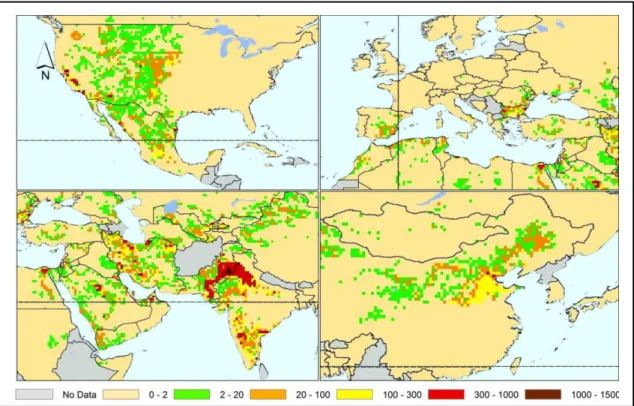
of groundwater extraction (bottom) (in mm/year modified from Wada et al., 2010)... 5 FIGURE 0.3: World map of simulated groundwater depletion in the regions of the U.S.A.,

Europe, China and India and the Middle East for the year 2000 (in mm/year modified from Wada et al., 2010) ... 6 FIGURE 1.2: Relationship between well yield and lithology in Niger (modified from UNESCO,

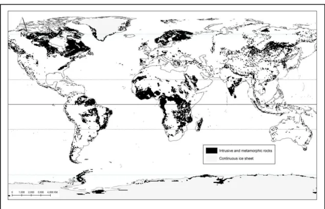
1999) ... 12 FIGURE 1.1: World map of crystalline rock distribution gridded to a 0.5fl spatial resolution

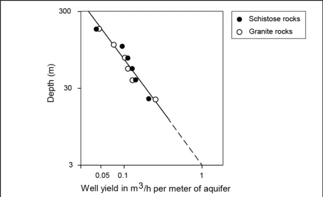
(data from Hartmann & Moosdorf, 2012)... 12 FIGURE 1.3: Global Groundwater Vulnerability to Floods and Droughts (Richts & Vrba, 2016)13 FIGURE 1.4: Relationship between well yield and depth in crystalline hard rocks of eastern

United States (modified from Davis & Turk, 1964) ... 14 FIGURE 1.5: Typical granite mineralogy ... 15 FIGURE 1.6: Relative displacements according to fracture type (modified from Martel, 2017) . 16 FIGURE 1.7: Photo of exfoliation joints on granite slopes (from Migoń, 2006) in Sierra Nevada,

California (left) and of spheroidal exfoliation of granite in the Kosciusko area in Australia (from Ollier, 1971; right) ... 17 FIGURE 1.8: Conceptual model of a crystalline aquifer, (a) under strong tectonic constraints

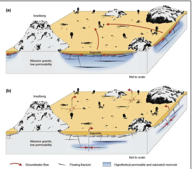
and (b) in tectonically stable, weathering-dominated areas (after Wyns et al., 2004 and Lachassagne, 2008) ... 18 FIGURE 1.9: Conceptual hydrogeological model for the weathered crystalline-basement aquifer

in Africa (modified from Chilton & Foster, 1995 and Singhal & Gupta, 2010) ... 21 FIGURE 1.10: Fracture-scale heterogeneities, illustrated by an example in diorite in Aspö,

Sweden (based on Winberg et al., 2000; modified from Guihéneuf, 2014) ... 22 FIGURE 1.11: Relationship between fracture density and hydraulic conductivity (modified from Maréchal et al., 2004) ... 23 FIGURE 1.12: Illustration of some techniques used to estimate transmissivity and storage

coefficient (T and S): (a) single borehole flowmeter test, (b) cross-borehole flowmeter test, and (c) long term pumping test with observation wells (modified from Le Borgne et al., 2006) ... 24 FIGURE 1.13: Relationship between scale of measurement and hydraulic conductivity (modified from Hsieh, 1998) ... 25 FIGURE 1.14: Schematic profiles of landforms in a crystalline rock terrain; note that

weathering patterns within the depositional landforms are not illustrated here (modified from Singhal & Gupta, 2010) ... 27 FIGURE 1.15: REV in different rock conditions: (a) homogeneous porous rock, (b) fractured

rock where REV includes sufficient fracture intersections, and (c) rocks with large scale discontinuities where REV is either very large or nonexistent (from Singhal & Gupta, 2010) ... 29 FIGURE 1.16: The three most common model concepts for numerical modelling of groundwater

flow and transport through a body of rock with fractures (modified from Swedish National Council for Nuclear Waste, 2001) ... 31

x

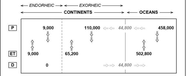
FIGURE 1.17: Conceptual groundwater flow model at the watershed-scale as a function of water level conditions: (a) under high water level conditions and (b) under low water level conditions (from Guihéneuf et al., 2014) ... 32 FIGURE 2.1: Schematic diagram of the hydrological cycle fluxes in km3_{/year (modified from}

Seiler & Gat, 2007); P refers to precipitation, ET to evapotranspiration and D to

discharge. ... 35 FIGURE 2.2: Schematic diagram of the hydrological cycle (from Singhal & Gupta, 2010) ... 37 FIGURE 2.3: Schematic cross-section of an aquifer situated on a circular island in a freshwater

lake being developed by pumping (modified from Bredehoeft, 2002) ... 39 FIGURE 2.4: Relationship between (a) depth of water table and rate of evaporation (modified

from Chen & Cai, 1995) and (b) depth of water table combined with terrain conditions on evapotranspiration (from Bouwer, 1978; modified by Singhal & Gupta, 2010) ... 41 FIGURE 2.5: A classification of process mechanisms in the response of hillslopes to rainfall; (a)

infiltration excess overland flow (Hortonian overland flow); (b) saturation excess overland flow (Dunne overland flow); (c) subsurface stormflow (event flow); (d) perched saturation and throughflow (modified from Beven, 2012) ... 43 FIGURE 2.6: Water movement in the unsaturated zone (modified from Dingman, 2015) ... 47 FIGURE 2.7: Soil-water status as a function of pressure. (modified from Miller & Donahue,

1990) ... 48 FIGURE 2.8: Classification of soil-hydrologic horizons. Note that this figure is not to scale (the

vertical extent of the unsaturated zone is exaggerated) and idealized and that any or several of these “horizons” might be absent under given conditions (modified from Alley et al., 1999 and Dingman, 2015). is the permanent wilting point, is field capacity.50 FIGURE 2.9: Typical infiltration rates over time for three soil columns (modified from Nimmo,

2005) ... 54 FIGURE 2.10: Typical forms of the moisture-characteristic curve ( − ) and the

moisture-conductivity curve ( − ); in this example porosity equals 0.5 (modified from

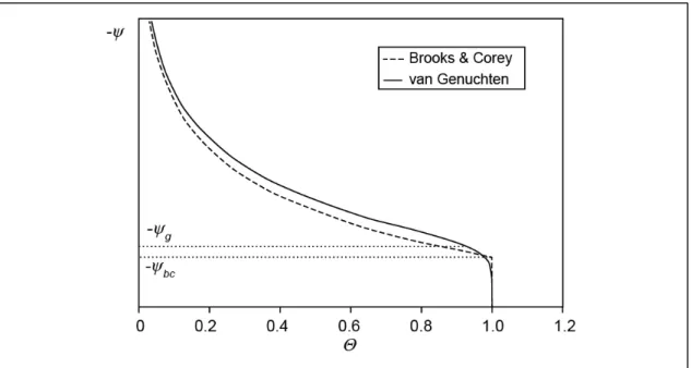
Dingman, 2015) ... 55 FIGURE 2.11: Typical moisture characteristic curves for the Brooks & Corey (1964) and van

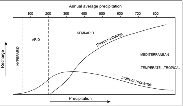
Genuchten (1980) models on a semi-log scale (modified from de Condappa, 2005) ... 58 FIGURE 2.12: The various mechanisms of recharge (modified from Saether & Caritat, 1996) .. 61 FIGURE 2.13: Recharge types in relation to general climatic conditions (modified from

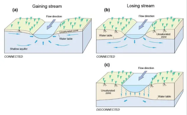
UNESCO, 1999)... 62 FIGURE 2.14: Different types of surface water/groundwater interactions: (a) a gaining stream

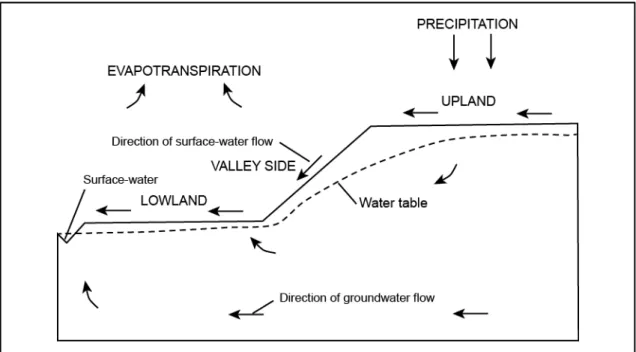
receiving water from the groundwater system, (b) a losing stream discharging water to the groundwater system, (c) a disconnected losing steam (modified from Winter et al., 1998) . 63 FIGURE 2.15: Fundamental hydrologic landscape unit (modified from Winter, 2001) ... 65 FIGURE 2.16: Low permeability aquifer with topography-controlled water-table (a) and highly

permeable aquifer with recharge controlled water-table (b) (modified from Haitjema & Mitchell-Bruker, 2005) ... 65 FIGURE 2.17: Groundwater resources map of the world (Richts et al., 2011) ... 66 FIGURE 3.1: Schematic groundwater balance for a drainage basin (modified from Dingman,

2015) ... 71 FIGURE 3.2: Schematic depth proles of the Cl concentration of soil water: (a) piston flow with

extraction of water by roots; (b) same as (a) but with preferred flow below the root zone or diffusive loss to the water table and (c) a profile reflecting past recharge conditions (modified from Allison et al., 1994) ... 77 FIGURE 3.3: Water fluxes related to the degree of connection between rivers and aquifers. The

aquifer discharges to the river when the groundwater head is greater than the river stage, and vice versa. Recharge values generally reach a constant rate when the water-table depth is greater than twice the river width (modified from Scanlon et al., 2002) ... 83

xi

FIGURE 3.4: Schematic representation of the use of piezometers and seepage meter to measure groundwater flux into (solid line) or out of (dashed line) a stream. Arrows indicate flow direction, dh is the head difference and dz is the elevation difference between the two piezometers. Vertical flow is calculated using Darcy’s law. Water flowing into or out of the container of the seepage meter is collected in the flexible ‘balloon’ (modified from

Dingman, 2015) ... 84 FIGURE 3.5: Range of fluxes that can be estimated using various techniques (from Scanlon et

al., 2002) ... 90 FIGURE 3.6: Spatial scales represented by various techniques for estimating recharge.

Point-scale estimates are represented by the range of 0 to 1 m (from Scanlon et al., 2002) ... 91 FIGURE 3.7: Time periods represented by recharge rates estimated using various techniques.

Time periods for unsaturated and saturated- zone tracers may extend beyond the range shown (from Scanlon et al., 2002) ... 91 FIGURE 4.1: (a) Methods to bring an aquifer to hydrologic equilibrium by either reducing

extraction or by increasing supply through MAR or through use of alternative supplies and (b) water stress reduction methods sorted by their relative costs and saved or supplied volumes (modified from Dillon et al., 2012) ... 100 FIGURE 4.2: Diagram of different artificial recharge methods (modified from Gale et al., 2002)106 FIGURE 4.3: Geometry and symbols for Green-and-Ampt piston flow model of infiltration

(based on Bouwer, 2002) ... 108 FIGURE 4.4: Schematic diagram of a groundwater mound forming beneath a hypothetical

infiltration basin and the relative shape of the mound in aquifers of higher and lower permeability (modified from Carleton, 2010) ... 109 FIGURE 4.5: Diagram showing managed aquifer recharge below a basin under (a) shallow

water table conditions and (b) deep water table conditions (modified from Bouwer, 2002)113 FIGURE 4.6: Dimensionless plot of seepage (expressed as I/K) and depth to groundwater

(expressed as DW/W) for a basin with no clogging layer at the bottom. I is the infiltration

rate and K is the hydraulic conductivity in the wetted zone. DW is the depth to the water

table and W is the width of the recharge system (modified from Bouwer, 2002) ... 116 FIGURE 4.7: Schematic representation of water level variations in response to artificial

recharge from an infiltration basin featuring parameters used in analytical modeling of artificial recharge (modified from Warner et al., 1989) ... 120 FIGURE 0.1: Map of the 29 states in India (union territories not shown) (a) and map of

climatic zones in India (modified from de Golbéry & Chappuis, 2012) (b) ... 133 FIGURE 0.2: Total population in India according to the World Bank

(https://data.worldbank.org/). Total population is based on the de facto definition of population, which counts all residents regardless of legal status or citizenship. The values shown are midyear estimates. ... 134 FIGURE 0.3: Annual mean rainfall (from Reddy et al., 2015) (a) and map of mean recharge for

the 1996-2015 period derived from water level measurements (from Bhanja et al., 2018); white areas are areas of no data availability (black lines are the main catchment

delimitations) (b) in India. ... 135 FIGURE 0.4: Baseline water stress in India according to the World Resources Institute

(https://www.indiawatertool.in/). Water stress is calculated on the basis of the amount of annually available surface water which is used every year. ... 136 FIGURE 0.5: Simplified geological map of India and the state of Telangana and location of

study sites used for this work. ... 137 FIGURE 5.1: Relative position of the Maheshwaram catchment within the state of Telangana

(India) and geological map of the Maheshwaram catchment, topography is shown as well as the main urban areas and percolation tanks. The location of scientific borewells which are currently equipped with a pressure probe to continuously measure water levels is also shown. ... 142

xii

FIGURE 5.2: Weathering profile of Maheshwaram area. Photos are of a dugwell located in the biotite granite, and show the upper part of the weathering profile. (modified from

Dewandel et al., 2006). ... 143 FIGURE 5.3: Daily precipitations (in mm/day) from 01/01/2000 to 31/05/2017 measured and

provided by ICRISAT (80 km north-east of Hyderabad) with a zoom on the period 06/2016 - 06/2017 to show the seasonal rainfall distribution. Yearly rainfall estimates are also provided (mm/yr). ... 144 FIGURE 5.4: Maximum and minimum temperatures from 01/01/2000 to 31/05/2017 measured

and provided by ICRISAT (80 km north-east of Hyderabad) ... 144 FIGURE 5.5: Seasonal piezometric maps for the year 2013 calculated from water levels in

scientific, abandoned and agricultural wells (white points) interpolated using standard kriging (model: spherical; length: 900 m; sill: 42.5). ... 145 FIGURE 5.6: Piezometric level above mean sea level (left axis) or water depth below ground

surface (right axis) at the IFP09 borewell at the Maheshwaram catchment from

17/01/2002 to 31/05/2017 (the full currently available time series); yearly rainfall is shown above to give an idea of the general hydrologic conditions prevailing each year. ... 146 FIGURE 5.7: Typical soil horizons (modified from unknown source). ... 147 FIGURE 5.8: Photos of observation trenches dug during field campaigns to assess the soil

hydraulic properties. The photos feature the different soil orders observed during the investigation carried out in de Condappa, (2005) (modified from de Condappa, 2005). .... 149 FIGURE 5.9: Map of soil type distribution at the Maheshwaram catchment (modified from de

Condappa, 2005). ... 149 FIGURE 5.10: Satellite data acquired by the American Earth observation satellite Landsat 8

and downloaded freely via Google Earth Engine (https://earthengine.google.com/). Acquisition dates correspond to Rabi season prior to harvest, on the left during a year when water levels were high (2014) and on the right a year when they were very low (2016). Areas of significant changes in paddy field extent were circled. ... 152 FIGURE 5.11: Land use map for the Rabi period (February 2003) initially from the National

Remote Sensing Agency (NRSA) but modified by de Condappa (2005) (a) and simplified land use distribution for use in the hydraulic model used to quantify recharge (b). ... 153 FIGURE 5.12: Reference recharge values computed for the Maheshwaram catchment using the

Double Water Table Fluctuation method for 2011 to 2015. Values are calculated at a resolution of 685×685 m, cell values were then interpolated using standard kriging

techniques (modified from Mizan, 2019). ... 154 FIGURE 5.13: Annual mean catchment recharge estimated using the DWTF method and the

theoretical linear rainfall-recharge relationship obtained performing a simple linear

regression; the rainfall-direct recharge relationship obtained experimentally by Rangarajan & Athavale (2000) is also shown (modified from Mizan, 2019). ... 155 FIGURE 5.14: Method to compute recharge from infiltration (modified from Dewandel et al.,

2008). ... 156 FIGURE 5.15: Schematic water balance at the parcel scale (concept from Dewandel et al., 2008,

format from Alley et al., 1999). Ω is the critical water depth above which runoff is

generated and L is the soil thickness. ... 158 FIGURE 5.16: Crop coefficients (KC ) for a few different land uses, some of which depend on

their agricultural calendar; ‘a’ is crop seeding, ‘b’ is crop harvesting (modified from

Dewandel et al., 2008 with data from de Condappa 2005)... 159 FIGURE 5.17: Variations in water volume for the period from 01/01/2000 to 04/12/2002 for a

total of 4722 days (a), daily water volume increase (b) in the Tumulur tank and Tumulur tank placement within the Maheshwaram catchment and in regards to the drainage

network. ... 160 FIGURE 5.18: Filtering process for choosing significant volume increases to calibrate the runoff

threshold. Volume increases below 750 m3_{/day are thus considered negligible. ... 161}

xiii

FIGURE 5.20: Simulated mean modelled runoff with Ω= 3 cm (bottom) and significant

volume increases in the Tumulur tank (top). ... 168 FIGURE 5.21: Yearly diffuse recharge (RI) values computed for the Maheshwaram catchment.

Values are calculated at a resolution of 100×100 m. ... 170 FIGURE 5.22: Rainfall and diffuse recharge variations computed for two different combinations

of soil type and land use: an Inceptisol with scrub vegetation against an Alfisol 2 with scrub vegetation (a) and an Entisol with a perennial paddy against an Entisol with scrub vegetation (b). Recharge from the Entisol with scrub vegetation may appear absent from the graph but is actually zero during the illustrated period. ... 171 FIGURE 5.23: Modelled catchment-scale yearly diffuse recharge values averaged over the

Maheshwaram catchment relative to rainfall and comparison with the total recharge trend relative to rainfall obtained from Mizan (2019). Each point corresponds to a given year; the simulation was run from 1995 to 2015 though only the years from 2000 to 2015 are shown. ... 172 FIGURE 5.24: Estimated yearly focused recharge plotted against rainfall for the 2011-2015

period (a) and modelled yearly runoff plotted against rainfall as well for the 2000-2015 period (b); both are in mm.yr-1_{. ... 175}

FIGURE 5.25: Raw difference between mean total recharge and mean diffuse recharge, assumed to be equal to focused recharge (a) and the same map with superimposed topography, drainage network, percolation tanks and geological boundaries in order to identify the possible contributors to focused recharge (b) ... 178 FIGURE 5.26: Sensitivity analysis of model parameters used to estimate diffuse recharge. This

analysis was performed by varying each parameter individually and comparing the outputs to a reference model run, chosen arbitrarily. is the texture dependent conductivity shape parameter [-], is the Brooks and Corey air entry pressure-head [L], is the saturated soil moisture content [-], is the saturated hydraulic conductivity [L.T-1_{], is the soil}

thickness [L] and is the runoff threshold [L]. Legend is sorted in order of importance. . 180 FIGURE 5.27: Summary diagram featuring the relationship between rainfall and recharge for

diffuse recharge, focused recharge (this study) and total recharge (from Mizan, 2019). Mean annual groundwater abstractions shown (174 mm/yr) are from Dewandel et al. (2010). ... 181 FIGURE 6.1: Study site location and position relative to Hyderabad (a, b), the Musi River and

the supply channel (c); borewell position within EHP site (d, e, f), orange points are those equipped with pressure sensors. ... 190 FIGURE 6.2: Hydraulic head variations in the CH03 borewell (longest on-site observed time

series) and rainfall. Recharge basin was first filled by the end of 2015 (black arrow). The horizontal gray line illustrates the limit between the saprolite and the granite determined from borehole cuttings. For information relating to technical specificities of the well, refer to Guihéneuf (2014) ... 191 FIGURE 6.3: Conceptual model of transmissivity ( ) and storativity ( ) profiles by depth

extrapolated from several hydraulic tests performed on-site by from Boisson, Guihéneuf et al. (2015) and schematic representation of geological log (modified from Boisson,

Guihéneuf et al., 2015)(Boisson, Guihéneuf et al., 2015). Storativity measurements end at the top of the fissured bedrock because they could not be measured within the saprolite at the time of the study as the boreholes are fully cased down to the contact between

saprolite and fissured bedrock ... 193 FIGURE 6.4: Basin water level variations (gray curve) and associated hydraulic head variations

in site boreholes shown in FIGURE 6.1. Only 3 boreholes are shown for clarity purposes, as variations between neighboring boreholes was very similar. ... 195 FIGURE 6.5: Schematic representation of water level variations in response to artificial

recharge from an infiltration basin featuring parameters used in analytical modeling of artificial recharge (adapted from Warner et al., 1989) ... 199

xiv

FIGURE 6.6: Model grid (a) and layer (b) configuration used for numerical modeling (modified from Chiang & Kinzelbach, 1992) with a conceptual 3D representation of the model’s two scenarios (c) ... 202 FIGURE 6.7: Infiltration relative to water levels in the basin for each phase of infiltration (a)

and proportionality coefficients between infiltration and basin water levels plotted as a function of time. Proportionality coefficients are obtained for each individual recession period following the equation = × (b). ... 203 FIGURE 6.8: Infiltration and canal inflow estimated for the observation period. Inflow is

episodic and short-lived as it is controlled by the opening and closing of an upstream floodgate managed by a third-party entity. ... 204 FIGURE 6.9: Recession slopes when the basin is fully connected to the aquifer (P3) at an

hourly time-step plotted on a semi-log axis where the slope is equal to – (a), and close-up of the shorter recession slopes (b). Each line corresponds to a different recession slope; five different recessions are shown. ... 205 FIGURE 6.10: Observed hydraulic head and simulated hydraulic head using analytical

modeling in response to infiltration from the recharge basin when it is disconnected from the water table (P1) for the boreholes closest to the basin (CH01 and CH02) ... 206 FIGURE 6.11: Simulated hydraulic head for the reference and compartmentalized scenario

under constant recharge ( = 10-6 _m.s-1_{), where the lateral extension of the compartment is}

varied (a) and where the vertical extension is varied (b). Set distance to basin is 100 m. = 10-4 _m.s-1 _{and = 10}-2 _{... 207}

FIGURE 6.12: Observed hydraulic head and simulated hydraulic head using numerical

modeling accounting for compartmentalization in response to infiltration from the recharge basin (gray lines) for the boreholes closes to the basin (CH01 and CH02) ... 208 FIGURE 6.13: Schematic representation of hydraulic head variations above the bedrock (gray

area) in response to artificial recharge from a recharge basin per phase of infiltration ... 209 FIGURE 6.14: Depth of the upper fissured layer from ERT surveys (a) and inferred 3D

conceptual model of structure (b). Hypothetical compartment delimitation is the thin black lines. For clarity purposes only the wells shown in FIGURE 1.4 are shown here. ... 211 FIGURE 6.15: Comparison of schematic representation of artificial recharge from an infiltration

xv

List of tables

TABLE 2.1: Estimate of global water distribution (percentages are rounded so will not add to 100) (from Oki, 2006) ... 34 TABLE 2.2: Approximate residence times in the main water reservoirs (from Gilli et al., 2016)36 TABLE 2.3: Classification of different forms of aridity (Cherlet et al., 2018) ... 40 TABLE 2.4: Classification of flow mechanisms that produce event responses (from Dingman,

2015). Processes underlined with a solid line pertain to the “direct runoff” category, and those underlined with a dashed line to “indirect runoff”. ... 42 TABLE 2.5: Environmental factors favoring some hillslope response mechanisms (modified from

Dingman, 2015) ... 46 TABLE 2.6: Analytic approximations of the ( ) and ( ) relations ... 58 TABLE 3.1: Representative values of porosity (Φ), specific yield (Sy) and specific retention (Sr)

(from Singhal & Gupta, 2010) ... 87 TABLE 4.1: Factors affecting MAR effectiveness in relation to hydrogeological setting

(modified from Gale et al., 2002) ... 111 TABLE 4.2: Characteristics of aquifers and their influence on MAR effectiveness (modified from Dillon & Jimenez, 2008) ... 112 TABLE 5.1: Mean water input values and field area from field investigations (from Dewandel et al., 2008, 2010). ... 161 TABLE 5.2: Mean soil hydraulic parameters for each soil type and a few specific land uses from

de Condappa (2005). Alf1. and Alf2. are Alfisols 1 and Alfisols 2, respectively, Incep. are Inceptisols, Ent. are Entisols and Tank refers to soils below the tank. ... 164 TABLE 5.3: Surfaces of each soil type and land use category and ratio between surfaces before

and after discretization. ... 166 TABLE 5.4: Number of days during which runoff was generated by the recharge model

depending on the runoff threshold selected from 01/01/2000 to 04/12/2012. ... 167 TABLE 5.5: Yearly components of the water budget averaged over the entire catchment area.

D represents runoff, RI is recharge from infiltration (diffuse recharge), AET is actual

evapotranspiration, RF is irrigation return flow, P is precipitation, PG is groundwater irrigation, Total w is the stock of water in the soil at the end of each year and ∆w is the change in soil moisture from the end of the prior year to the end of the year in question. All components are in mm.yr-1_{. ... 174}

TABLE 6.1: Boreholes characteristics of the Experimental Hydrogeological Park in Choutuppal (Andhra Pradesh, Southern India) from Guihéneuf et al. (2014). Boreholes location is provided in the UTM projected coordinate system. Borehole depth and casing depth are given in meters below ground surface. ... 194 TABLE 6.2: Contributions of water budget components ... 204 TABLE 6.3: Hydraulic properties obtained from calibration of analytical simulations to

xvi

“Hard rock hydrogeologists, the world over, are therefore divided into two main groups: those interested in obtaining ground water for domestic, irrigational or industrial use by exploring fractured and permeable zones in a relatively less permeable matrix of hard rock, and those interested in locating impermeable or the least permeable zones for storage of hazardous nuclear waste.

Ironically, for the first group even the most permeable zones are often not good enough to yield adequate water supply, while for the second group even the least permeable zones are often not good enough for safe storage of hazardous nuclear waste over a prolonged period of a few hundred years.”

1

Introduction

The Industrial and Technological Revolution

In a rapidly industrializing world, challenges regarding water are incessantly increas-ing. Explosive population growth, combined with a strong expansion of irrigated agricul-ture and industrial development, are adding stress on the quality and quantity of natural systems. Prior to the Industrial Revolution of the late eighteenth and nineteenth centu-ry, both population growth and living standards remained relatively static (Harris & Roach, 2018). Thereafter, rapid technological progress and the advent of the market economy set off a staggering population growth that significantly altered established patterns. This led British economist Thomas Malthus, in 1798, to propose the hypothe-sis that: “The power of population is indefinitely greater than the power in the earth to produce subsistence for man” (p. 9), i.e. populations were bound to outgrow their food supplies. During the period that followed, while thousands of individuals continued to be victims of drought and famine, mankind as a whole has disproved the Malthusian hy-pothesis. Although the world’s population has skyrocketed from one to over seven billion in the last 200 years, economic output per person has in fact grown and living standards have risen, even in the face of significant and increasing inequality (Harris & Roach, 2018). However, the essential core of the Malthusian argument remains valid–growing human populations and economic systems can outrun their biophysical support systems. In fact, over the past few decades, the scope and urgency of issues related to increasing resource demands have become a central focus of global awareness and efforts to miti-gate environmental degradation. During the 1992 United Nations Conference on Envi-ronment and Development (UNCED), attention was focused on the major global issues threatening mankind: the depletion of the ozone layer, destruction of forests and wet-lands, major species extinction and the steady build-up of greenhouse gases causing cli-mate change. Twenty years later, countries of the world reaffirmed their commitment to including environmental issues in their development goals at the United Nations Rio +20 Conference. However, the 2012 United Nations Environment Program (UNEP) report found that, with the exception of ozone depletion, all of the global environmental prob-lems identified at UNCED have continued or worsened. In fact, further UNEP reports have identified increasingly destructive side-effects of indiscriminate economic growth, many of which impact our freshwater sources (e.g. eutrophication and acidification of aquatic systems, declining groundwater supplies, overexploitation of ocean and freshwa-ter ecosystems, etc.).

2

Groundwater, which accounts for by far the largest volume of unfrozen freshwater on Earth, is among the most important of our natural resources. Compared with surface water, groundwater is of higher quality, better protected from pollution, less subject to seasonal and perennial fluctuations, and much more uniformly distributed across large regions. Furthermore, considering the increasing variability of water supplies, especially under climate change, groundwater constitutes a crucial buffer in coping with current and upcoming environmental challenges. These advantages, combined with the fact that groundwater is for some countries (e.g. Saudi Arabia, Malta, Denmark) the only or most important source of water, have made groundwater the most exploited resource on earth (UNESCO, 2004). Over the past decades, groundwater use in agricultural and other eco-nomic sectors has soared, contributing to massive improvements in the quality of life in many parts of the world. As such, it has served as one of the largest and most potent modes of poverty reduction in recent decades (Sharma et al., 2005).

The Silent Revolution

Irrigation is the most important water use sector, especially in arid and semiarid cli-mates, accounting for 70% of global freshwater withdrawals and 90% of consumptive water uses (Siebert et al., 2010). The spectacular increase in groundwater use that has led to the current situation began in the twentieth century, during a phenomenon that has been called “the Silent Revolution” (Llamas & Martínez-Santos, 2005a). At the start of the century, the boom in groundwater development was limited to a few countries, with Italy, Mexico, Spain and the United States among the leaders. A second wave be-gan later, in the 1970s, in South Asia, parts of China, the Middle East and northern Africa, and continues today (Van der Gun, 2012). Overall, since the 1950s, groundwater use, most significantly for irrigation, has significantly increased in many parts of the world (FIGURE 0.1). In Spain, it has increased from 2 km3_{/year to 6.5 km}3_/year, ac-counting for 15-20% of all water used in the country (Hernández-Mora et al., 2010). In the United States, groundwater use for irrigation increased from 23% in 1950 to 48% (i.e. 46 to 113 km3_{/year) of total freshwater withdrawals in 2015 (Dieter et al., 2018). In} In-dia, groundwater use has soared from 10-20 km3_{/year before 1950 to a} world-record-breaking over 250 km3_{/year today (Siebert et al., 2010), making India by far the largest} exploiter of groundwater on earth. Yearly abstractions in India are more than double those of the second runner-up, China, whose yearly abstractions average about 110 km3_{/year (Van der Gun, 2012), despite China’s greater population. This is due to an} interplay of factors, such as the implementation by the Chinese government of a metered tariff regime, and an overall lesser dependence on groundwater (in India 55-60% of the population depends on groundwater vs. 22-25% in China) (T. Shah et al., 2003). In sub-humid to arid areas, specifically, groundwater abstraction has increased from 126 (± 32) km3 _{in 1960 to 283 (± 40) km}3 _{in 2000 (Wada et al., 2010). While in the US, Spain,}

Introduction

3 Mexico and North-African countries like Tunisia or Morocco total groundwater use peaked during the 1980s or thereabouts, and has since decreased, in South Asia and parts of China the upward trend that began during the 1970s is still ongoing. Further-more, it is predicted there will likely be a third wave of exponential growth in groundwa-ter abstraction in many regions of Africa and some southeast Asian countries such as Vietnam and Sri Lanka (Molle et al., 2003).

This worldwide boom can be attributed largely to numerous individual decisions by millions of modest farmers pursuing the significant short-term benefits to be derived from groundwater use. Decisions were made without centralized planning or coordina-tion; this is why it is called “the Silent Revolution”. Technological and scientific ad-vancements are at the core of this “Revolution”. Improvement in well-drilling techniques, advancements in hydrogeology and the popularization of the submersible pump dramati-cally reduced abstraction costs. Today, the total cost of groundwater abstraction is only a small fraction of the economic value of the guaranteed crop. This has allowed farmers to progressively shift from low-value crops to cash crops, which are also more water-intensive. As an example, a hectare of cereal can be valued at around USD$500, while tomatoes or cucumber can be worth more than USD$60,000, i.e. over 100 times more valuable (Llamas & Martínez-Santos, 2005a). Although water use by these farmers has frequently been incentivized by soft loans or energy subsidies from governmental sources, most governmental agencies have overlooked the real effects and extent of groundwater development. Instead, they have focused mainly on the maintenance and control of sur-face water (Llamas & Martínez-Santos, 2005a). However, despite the fact that govern-FIGURE 0.1: Approximate groundwater abstraction trends in selected countries (in km3/year modified from Shah, 2005 and Van der Gun, 2012)

4

mental subsidization of surface water often makes it cheaper than groundwater, many farmers prefer groundwater. There are several reasons for this choice: first, groundwater can be obtained individually, thus bypassing often time-consuming negotiations with other farmers and government officials (Llamas & Martínez-Santos, 2005a). Second, and most important, groundwater is more resilient in dry periods and more generally availa-ble (as opposed to surface water). In practice, most farmers rely on the conjunctive use of surface water and groundwater, assuming the latter is readily available.

The combination of an exponential increase in individual borewells and the lack or ineffectiveness of regulation has led to adverse effects in places like South Asia, where the current situation has been described as “colossal anarchy” (T. Shah, 2005). Indeed, this sudden boom in groundwater exploitation has triggered a series of harmful side ef-fects (Sharma et al., 2005): groundwater level declines leading to wells running dry, ris-ing energy and pumpris-ing costs, and growris-ing vulnerability to drought (Castle et al., 2014; Famiglietti, 2014; Scanlon et al., 2012; Van Loon et al., 2016), saltwater intrusion in coastal areas (Werner et al., 2013), and health hazards derived from the aquifer itself (e.g. arsenic and fluoride contaminations) (Amini, Abbaspour et al., 2008; Amini, Mueller et al., 2008; Chuah et al., 2016; Rodriguez-Lado et al., 2013) or external sources including agriculturally derived chemicals (Böhlke, 2002; Hallberg, 1989; Pimentel et al., 1992; Rattan et al., 2005; Spalding & Exner, 1993). In many parts of the world, ground-water abstractions exceed natural groundground-water recharge, which has caused overexploita-tion and persistent groundwater depleoverexploita-tion in these regions (FIGURE 0.2 and FIGURE 0.3). Among the current “hot-spots” of groundwater depletion worldwide, the most no-table are Pakistan, India (see also Rodell et al., 2009), North-East China, central U.S. and California, Yemen and Spain (FIGURE 0.3).

Introduction

5 FIGURE 0.2: World map of simulated average groundwater recharge (top) and of the inten-sity of groundwater extraction (bottom) (in mm/year modified from Wada et al., 2010)

6

On the importance of crystalline rock aquifers

Countries situated in arid and semiarid regions are the most dependent on ground-water for their ground-water supply. However, a substantial area of the semiarid and arid re-gions of the world is underlain by crystalline rock in which the bulk of the available groundwater is found. Conservation management and planning of water resources is par-ticularly challenging in these environments. This is because crystalline rock aquifers are characterized by their extremely low primary hydraulic conductivities and porosities, regardless of their origin or lithological type (UNESCO, 1999), which makes them very little receptive to the transmission and storage of water. Further, crystalline rock aqui-fers are complex geological formations; aquiaqui-fers are often compartmentalized (Ayraud et al., 2008; Guihéneuf et al., 2014; Perrin et al., 2011; Roques et al., 2014), and their hy-draulic properties vary very widely, both vertically and horizontally, due to the media’s intrinsic heterogeneity (Acworth, 1987; Boisson, Guihéneuf et al., 2015; Chilton & Foster, 1995; Dewandel et al., 2012; Maréchal et al., 2004). These disadvantages are fur-ther accentuated in arid and semiarid climates. First, because storage is essential in wa-ter-scarce areas, yet as mentioned above, igneous and metamorphic rocks do not permit a sizeable subsurface storage of groundwater (UNESCO, 1999). Second, because dry con-ditions compounded with the high variability of rainfall events leads to non-linear re-charge patterns which are heavily biased to heavy rainfall events (Taylor et al., 2012). FIGURE 0.3: World map of simulated groundwater depletion in the regions of the U.S.A., Europe, China and India and the Middle East for the year 2000 (in mm/year modified from Wada et al., 2010)

Introduction

7 Also, as aridity increases, direct recharge becomes less important than localized and indi-rect recharge (i.e. through the beds of surface-water bodies, and depressions joints and rivulets) (de Vries & Simmers, 2002), which is more difficult to quantify and less spread-out.

The fact that crystalline rock aquifers are poor water reservoirs can dampen the agri-cultural development potential of the regions that rely on them and prevent them from attaining the level of socio-economic affluence enjoyed by other regions that have access to sustainable and reliable water supplies (UNESCO, 1999). Despite the existing research in this field, groundwater flow and transport in crystalline rock are still not fully under-stood. To give a few examples, the processes that control recharge quantities and distri-bution (in both time and space) in crystalline environments remain of keen interest in the scientific community (e.g. Clark & Douglas, 2000; Gleeson et al., 2009; Jiménez-Martínez et al., 2013; Neves & Morales, 2007; J Perrin et al., 2012; Rohde et al., 2015). Similarly, determining the limits of admissible groundwater withdrawal (or artificial storage potentials) is still a matter of widespread debate (e.g. Hammond, 2018; Piscopo & Summa, 2007; Sarma & Xu, 2014; Van Tonder et al., 2001); and the study of pollu-tant and tracer transfer dynamics in these environments still provides fertile ground for current and future research (e.g. Guihéneuf et al., 2017; Levison & Novakowski, 2012; MacQuarrie & Mayer, 2005; Shapiro, 2001; see Neuman, 2005).

India, where about two thirds of the geographical areas are underlain by hard rocks, best exemplifies the challenges and implications characteristic of fractured crystalline rock water resources. Unfortunately, this country has become infamous for having some of the world’s most severe aquifer over-exploitation problems in the world (Rodell et al., 2009; T. Shah et al., 2012) with the result that 54% of the territory faces high to ex-tremely high water stress (Shiao et al., 2015).

The Indo-French Centre for Groundwater Research

It is in this context that the Indo-French Center for Groundwater Research (IFCGR) was created in 1999. It is the result of cooperation between the French geologi-cal survey (or BRGM, Bureau de Recherches Géologiques et Minières) and the National Geophysical Research Institute (NGRI). The IFCGR is situated within the NGRI cam-pus in Hyderabad, the capital of the state of Telangana. One of the main objectives of this collaboration is to better understand hydrogeological processes in fractured crystal-line rock. To date, a substantial amount of data has been obtained by instrumenting and monitoring at different scales several sites in Archean granitic terrain, two of which were used for this thesis (see Maréchal et al., 2018).

The first is the Maheshwaram catchment, situated South-East of Hyderabad. It co-vers an area of 53 km2_{, and represents a typical inhabited catchment in granitic terrain.}

8

The many field surveys and publications carried out at this site since its establishment have allowed researchers to ascertain many of its characteristics (such as the hydraulic properties of the aquifer and its overlying soils, its geology and aquifer structure, and many others) greatly facilitating the elaboration and validation of models and hypothe-ses for medium to large-scale proceshypothe-ses.

The second is the Choutuppal experimental site, a highly instrumented and continu-ously monitored observatory. This site is equipped with 30 borewells over a surface of about 40 hectares, and allows the detailed analysis of medium to small-scale processes. As with the Maheshwaram catchment, previous studies have provided a good estimation of the site’s characteristics and hydraulic properties. In 2016 the latter was equipped with a Managed Aquifer Recharge (MAR) basin. This basin was built as part of a much broader project launched by the Indian government, which aims to alleviate groundwater overexploitation. To do so, the aim is to increase aquifer recharge from 9% of total rain-fall under natural conditions to 15% by 2020 (Government of Andhra Pradesh, 2003) through the development of large-scale MAR schemes. The Central Ground Water Board has proposed the building of 11 million MAR structures nation-wide, as well as the reparation, renovation and restoration of the already existing structures, the total costs tallying up to over 12bn USD (Central Ground Water Board, 2013). The Choutuppal site thus provides an exceptional opportunity to study the efficiency of this remediation technique and the potential of crystalline aquifers as artificial reservoirs.

Objectives

This thesis focuses specifically on the problem of recharge which is among the most important components of the groundwater budget. Analyzing, quantifying and mapping recharge processes is essential to both better our understanding of fractured crystalline rock aquifers and for the improvement of groundwater management strategies. For ex-ample, the study of recharge can help in defining sustainable yields and storage poten-tials, in the prevention of groundwater pollution, and can assist in the location of high and low yielding areas to optimize borewell and MAR placement. The overarching goal of this research is to improve our understanding of recharge, both natural and artificial, in fractured crystalline aquifers under semi-arid conditions and weathering processes. To that end, data from present-day monitoring, and datasets and outputs from previous studies were combined to produce an up-to-date detailed analysis of the factors control-ling recharge distribution and water flow propagation at medium and large scales. Nu-merical and analytical models were used to integrate the different sets of available data into saturated and unsaturated hydrogeological models of varying complexity, which in turn allowed us to better understand how and where recharge occurs in heterogeneous fractured media.

9

Part I

THEORETICAL DESCRIPTION

OF NATURAL AND ARTIFICIAL

RECHARGE IN FRACTURED

CRYSTALLINE ROCK

11

Chapter 1

Groundwater resources in

fractured crystalline rock

Geography of fractured crystalline rocks

1.

A large portion of the earth’s surface (about 34%; Blatt & Jones, 1975) features igne-ous and/or metamorphic rocks (i.e. crystalline rocks) which outcrop or lie close to the surface under a thin layer of alluvial or glacial deposits (FIGURE 1.1; Larsson, 1984). These outcrops are particularly present in the vast Precambrian shields which are locat-ed in every continent; they occur in the American continent (Canada, Northwest of the United States, Brazil…), Asia (South India and Sri Lanka, China, Siberia…) in northern Europe (most importantly in the Scandinavian countries), central and eastern Africa, and the Pacific region. For countries situated in temperate climates with abundant and high-quality surface water, problems linked to crystalline rock as a groundwater reservoir are of little importance. Although groundwater may still be exploited in these regions, other uses of crystalline rock such as exploitation for their mineral wealth or as a build-ing stone, or their use for storage of hazardous nuclear and chemical waste, may garner more attention. We can, for example, cite experiments performed to assess the potential for nuclear waste repository in several such regions: in the Canadian Shield (e.g. works from the URL in Canada; see Fairhurst, 2004), in the Fennoscandian shield (e.g. the Stripa Project; see Nordstrom et al., 1989), or at the Kamaishi Mine in Japan (e.g. Nguyen et al., 2001).

Nevertheless, large parts of the crystalline geological domain are located in tropical and subtropical regions where many developing countries are situated. In these cases, crystalline rock aquifers are often the only perennial source of groundwater. This is espe-cially the case in northeastern Brazil, India, western Africa (from Senegal to Cameroon), the Red sea region, and parts of the highlands of central and eastern Africa. In these regions, the lack of reliable water supplies has acted against economic and social devel-opment by impeding proper agricultural develdevel-opment and by dampening the potential of other industries (such as mining) which require large amounts of processing water (Larsson, 1984). This is because compared to other types of aquifers, borewell yields in fractured crystalline environments are quite modest (from less than 2-3 m3_{/h up to 20} m3_{/h; Ahmed et al., 2008; FIGURE 1.2). Some cases have been found where major} tec-tonic structures provide pathways for significant flow to take place (e.g. Neves & Morales, 2007; Roques et al., 2016; Seebeck et al., 2014), but these remain exceptions,

12

especially in the vast tectonically stable Precambrian shields. Despite this, their wide-spread presence makes them well suited to scattered settlements and small to medium cities, and has allowed certain regions to benefit from their use by contributing to the development of irrigated agriculture where surface water is limited.

FIGURE 1.1: World map of crystalline rock distribution gridded to a 0.5° spatial resolution (data from Hartmann & Moosdorf, 2012)

FIGURE 1.2: Relationship between well yield and lithology in Niger (modified from UNESCO, 1999)

Groundwater resources in fractured crystalline rock

13 FIGURE 1.3: Global Groundwater Vulnerability to Floods and Droughts (Richts & Vrba, 2016)

From an environmental perspective, however, these regions are among the most frag-ile parts of the world (FIGURE 1.3), which puts the livelihoods of millions of people at risk. Aside from mismanagement of crystalline aquifers due to sociopolitical reasons, it is some of the hydrodynamic characteristic features of crystalline aquifers which make them most vulnerable to overexploitation and contamination. Irrespective of their origin or lithological type, crystalline rocks are defined by (see Larsson, 1984; National Research Council, 1996; Singhal & Gupta, 2010; UNESCO, 1999): (i) extremely low pri-mary hydraulic conductivities and porosities (ii) strong heterogeneity of hydraulic pa-rameters in time and space which leads to compartmentalization and formation of pref-erential flow pathways (iii) shallow occurrence of water in useful quantities which de-creases in depth (FIGURE 1.4) (iv) generally poor yields (where drawdown in pumping wells is often almost equal to the saturated thickness of the aquifer). In sum, groundwa-ter occurrence in crystalline rocks is hegroundwa-terogeneous, complex, and overall not very signifi-cant. The non-receptiveness of these aquifers to the ready receipt, transmission and stor-age of water (and thus resistance to recharge) makes them specifically vulnerable to overexploitation, while their strong heterogeneity and complexity hinders the manage-ment and implemanage-mentation of responsible and sustainable water resource exploitation strategies.

14

Geology of fractured crystalline rocks

2.

Definition

2.1.

Crystalline rocks are composed almost entirely of crystallized minerals without glassy matter. Intrusive igneous rocks, those that congeal at depth, and metamorphic rocks, resulting from the transformation of preexisting rocks subjected to great heat and pres-sure, are virtually always crystalline. This thesis will focus specifically on intrusive igne-ous rocks. Also termed plutonic rocks, these rocks are formed from magma that cools and solidifies within the Earth’s crust, where temperatures and pressures are much high-er than at its surface. This leads the hot magma to cool slowly and crystallize complete-ly, thus prompting the growth of minerals large enough to be identified visually with a microscope (i.e. phenocrysts; FIGURE 1.5). Intrusive igneous rocks are composed of many kinds of minerals, but the dominant ones are invariably quartz, plagioclase feld-spar, and potassium feldspar (Migoń, 2006). Minerals of the mica group, muscovite and biotite, often occur in significant proportions as well. These rocks are exposed at the surface after long periods of weathering and erosion or by tectonic forces that may push the crust upward (or a combination of the two).

FIGURE 1.4: Relationship between well yield and depth in crystalline hard rocks of eastern United States (modified from Davis & Turk, 1964)

Groundwater resources in fractured crystalline rock

15 Because of the size and contiguous disposition of crystals, plutonic rocks have negli-gible intergranular spacing, which is associated with almost neglinegli-gible primary porosities and permeabilities: the matrix (the assemblage forming the intact rock) thus cannot con-tribute to groundwater resources in any meaningful way. Flow and storage in plutonic rocks is only possible if the rock undergoes chemical and physical modifications leading to the formation of fractures within these rocks (i.e. a secondary porosity) whose porosi-ty is much higher than the rock’s intrinsic primary porosiporosi-ty. The formation of a second-ary porosity allows water to penetrate into the rock in sufficient amount for it to even-tually be considered a reservoir.

Crystalline rock fracturing

2.2.

Fractures are mechanical failures in rock that occur when local stresses exceed the breaking point of a given rock. The term “fracture” is a generic term that denotes all discontinuities within the rock, regardless of their size (which can range from under a millimeter to several hundred kilometers). There are two types of brittle fractures (FIGURE 1.6), tensile, when the displacement develops perpendicular to the surface of displacement (mode I), or shear, when the displacement develops tangentially to the surface of displacement (mode II and III).

The two main fracture-forming processes in hard rock are:

₋ Weathering is a chemical and mineralogical modification of the rock under favor-able temperature and precipitation conditions, decreasing the cohesion of materi-als leading to fissuring of the material. By causing the dissolution and evacuation of the most soluble cations, weathering causes a change in mineralogical phases leading to the formation of clayey minerals. These minerals will then generate stress as they occupy more space than the original mineral, which will in term shatter the rock. The degree of weathering is dependent on the interplay of nu-merous factors, either relating to the rock itself (such as the relative surface area of the rock and its modification by mechanical weathering, the permeability of FIGURE 1.5: Typical granite miner-alogy

16

the rock mass, its mineralogical composition…) or to the external forces driving the weathering (such as the composition, amount and distribution of percolating water, the position of the water table, the activity of the macro- and microflora and fauna in the system…) (Larsson, 1984). Weathering-related fissures form or-thogonally to the weakest stress (in most cases sub-horizontally) and decrease from the top downward, generally becoming non-existent at about 50 m deep (Dewandel et al., 2006; Wyns et al., 2004).

₋ Tectonic fracturing is the formation of brittle fractures when the rock is submit-ted to mechanical stresses. The control of the type, distribution and degree of opening of tectonic fractures depends on their formation mechanism and their orientation with respect to the current stress field (Ashby & Hallam, 1986). The tectonic stress field consists of three principal comprehensive stresses, two of which are near the horizontal, and the third, due to the overburden load, near the vertical. The exact relationship between tectonic stress and the degree of fracture opening is however disputed, especially in the subsurface (i.e. <100 m depth), as it may be masked by other factors, such as topographic effects (St. Clair et al., 2015).

In tectonically stable regions (like shield zones) the most commonly encountered frac-tures are mainly opening-mode (mode I) fracfrac-tures which are parallel to topography. These fractures, also called exfoliation joints, break down the rock into a typical foliated structure which makes up the fissured zone of the aquifer. The foliation provides greater surface areas for subsequent chemical and physical weathering to take place, contrib-uting to further breaking down the rock. This, in term, can lead to the in-situ formation of a layer of loose, heterogeneous superficial deposits called saprolite, which is the ulti-FIGURE 1.6: Relative displacements according to fracture type (modified from Martel, 2017)