Humidity observations in the Arctic troposphere over Ny-Ålesund, Svalbard based on 14 years of radiosonde data

(1)

HAL Id: hal-00302541

https://hal.archives-ouvertes.fr/hal-00302541

Submitted on 25 Jan 2007

HAL is a multi-disciplinary open access

archive for the deposit and dissemination of sci-entific research documents, whether they are pub-lished or not. The documents may come from teaching and research institutions in France or abroad, or from public or private research centers.

L’archive ouverte pluridisciplinaire HAL, est destinée au dépôt et à la diffusion de documents scientifiques de niveau recherche, publiés ou non, émanant des établissements d’enseignement et de recherche français ou étrangers, des laboratoires publics ou privés.

Humidity observations in the Arctic troposphere over

Ny-Ålesund, Svalbard based on 14 years of radiosonde

data

R. Treffeisen, R. Krejci, J. Ström, A. C. Engvall, A. Herber, L. W. Thomason

To cite this version:

R. Treffeisen, R. Krejci, J. Ström, A. C. Engvall, A. Herber, et al.. Humidity observations in the Arctic troposphere over Ny-Ålesund, Svalbard based on 14 years of radiosonde data. Atmospheric Chemistry and Physics Discussions, European Geosciences Union, 2007, 7 (1), pp.1261-1293. �hal-00302541�

(2)

ACPD

7, 1261–1293, 2007

Humidity observations in the

Arctic troposphere over Ny- ˚Alesund

R. Treffeisen Title Page Abstract Introduction Conclusions References Tables Figures ◭ ◮ ◭ ◮ Back Close

Full Screen / Esc

Printer-friendly Version Interactive Discussion

Atmos. Chem. Phys. Discuss., 7, 1261–1293, 2007 www.atmos-chem-phys-discuss.net/7/1261/2007/ © Author(s) 2007. This work is licensed

under a Creative Commons License.

Atmospheric Chemistry and Physics Discussions

Humidity observations in the Arctic

troposphere over Ny- ˚

Alesund, Svalbard

based on 14 years of radiosonde data

R. Treffeisen1, R. Krejci2, J. Str ¨om3, A. C. Engvall4, A. Herber4, and L. W. Thomason5

1

Alfred Wegner Institute for Polar and Marine Research, Telegrafenberg A45, 14473 Potsdam, Germany

2

Department of Meteorology (MISU), Stockholm University, S 106 91 Stockholm, Sweden

3

ITM – Department of Applied Environmental Science, Stockholm University, S 106 91 Stockholm, Sweden

4

Alfred Wegner Institute for Polar and Marine Research, Am Handelshafen 12, 27570 Bremerhaven, Germany

5

NASA Langley Research Center Hampton, VA 23681-2199, USA

Received: 30 November 2006 – Accepted: 16 January 2007 – Published: 25 January 2007 Correspondence to: R. Treffeisen (renate.treffeisen@awi.de)

(3)

ACPD

7, 1261–1293, 2007

Full Screen / Esc

Abstract

Water vapour is an important component in the radiative balance of the polar atmo-sphere. We present a study covering fourteen-years of data of tropopsheric humidity profiles measured with standard radiosondes at Ny- ˚Alesund (78◦55′N 11◦52′E) during the period from 1991 to 2005. It is well known that relative humidity measurements

5

are less reliable at cold temperatures when measured with standard radiosondes. The data were corrected for errors and used to determine key characteristic features of the vertical and temporal RH evolution in the Arctic troposphere over Ny- ˚Alesund. We present frequency occurrence of ice-supersaturation layers in the troposphere, their vertical span, temperature and statistical distribution. Supersaturation with respect to

10

ice shows a clear seasonal behaviour. In winter (October–February) it occurred in 22% of all cases and less frequently in spring (March–May 13%), and summer (June– September, 10%). The results are finally compared with findings from the SAGE II satellite instrument on subvisible clouds.

1 Introduction

15

Climatological data sets of the water vapour distribution in the troposphere for low and mid-latitudes have been produced through the use of diverse data sources including radiosondes and satellite instruments. On the other hand, there is no similarly compre-hensive water vapour data set available for high latitudes. Nadir-viewing satellite-based techniques are limited at high latitudes due to the bright ice surface and the generally

20

dry Arctic conditions (Bates and Jackson, 2001; Randel et al., 1996). The standard instrument for in situ measurement of tropospheric water vapour is the radiosonde, but stations in the Arctic are sparse. In general, the accuracy and reliability of radiosonde RH measurements decrease as the water vapour concentration, temperature, or pres-sure decreases (Elliott and Gaffen, 1991). For instance, radiosonde data is limited

25

by the typically cold and dry Arctic environment as they tend to underestimate wa-1262

(4)

ACPD

7, 1261–1293, 2007

Full Screen / Esc

ter vapour at cold temperatures. Miloshevich et al. (2001) showed that the Vaisala RS80-A radiosonde exhibits a strong bias toward low relative humidity (RH) values at low temperatures. Radiosonde RH measurements in the stratosphere are considered to be essentially useless (WMO 1996; Schmidlin and Ivanov, 1998), in part because uncertainty in measurement generally exceeds typical stratospheric humidity of a few

5

percent RH.

Even with its limitations, radiosondes provide crucial water vapour data set for the Arctic free troposphere. It is of vital importance to climate research as water vapour has a major influence on radiative transfer in this region. Murphy et al. (1990), in their analysis of aircraft data in the winter-time Arctic, showed that ice saturation was not

un-10

common within 2 km of the tropopause due to the absence of ice nuclei (e.g. Gierens et al., 2004 and references therein). Cirrus clouds are widely recognised as a major component in energy budget regulation of the Earth-atmosphere system (Liou, 1986), yet the magnitude of cirrus climate forcing remains highly uncertain, despite consider-able efforts to quantify it (Stephens et al., 1990; Baker, 1997). It has been estimated

15

that cirrus clouds cover about 30% of the Earth’s surface (Wylie et al., 1994). SAGE II extinction observations of zonally averaged occurrence frequencies of the very thin clouds known as subvisible cirrus (SVC) clouds are given by Wang et al. (1996) for lat-itudes ranging from 60◦S to 60◦N. The measured 6-year of data clearly demonstrates the existence of such clouds in this entire latitude band, both above and below the

av-20

erage tropopause location, with an occurrence frequency maximum in the tropics. In this paper we present an analysis of a unique, long-term dataset of humidity profiles inferred from routine radiosonde measurements carried out in Ny- ˚Alesund, Svalbard.

The goal of this study is (1) to achieve a statistical presentation of the vertical and temporal distribution of the humidity above this high latitude Arctic location; (2) to

de-25

termine potential layers for the formation of high level ice clouds based on soundings and derive information about the geometry (height and depth) of these layers and to evaluate the results; (3) to compare the results obtained to long-term SAGE II mea-surements of subvisible clouds.

(5)

ACPD

7, 1261–1293, 2007

Full Screen / Esc

2 Data description

In this study we will make use of the radiosonde data and of measurements of subvisi-ble clouds from satellite data. These two sets of data are introduced below.

2.1 RH measurements from routine radiosonde data

Since October 1991 Vaisala radiosondes have been routinely launched from

Ny-5 ˚ Alesund (78◦ 55′ N 11◦ 52′

E). In this study we have used data from the period mid October 1991 up to December 2005. The radiosondes are launched daily at 11 a.m. UTC. Occasionally, during special programs, multiple radiosonde launches are made per day. Altogether 5314 profiles were analysed during the period 1991 to 2005. All profiles were corrected and averaged in 200 m steps and were restricted to values

10

up to 2 km above the tropopause height (RH measurements with radiosondes in the stratosphere are highly unreliable and not of interest within this study, see section 3 for details). The tropopause height from the radiosondes was determined by WMO standard methodology (WMO, 1996).

The radiosondes deliver profiles of temperature, relative humidity, wind speed and

15

wind direction. The principle of humidity measurement of Vaisala Humicap sensor is based on properties of a thin humidity sensitive polymer film placed between two electrodes. The film either absorbs or desorbs water vapour as the relative humidity changes. The dielectric properties of the polymer film depend on the amount of water contained, accordingly the dielectric properties of film change as does the capacitance

20

of the sensor. The electronics of the instrument measure the capacitance of the sen-sor and convert it to a humidity reading (http://www.vaisala.com/). Prior to July 2002 RS80-A radiosondes were used. The RS90 was used between July 2002 and sum-mer 2005 when the use of radiosonde type RS92 was initiated. The operation with the RS92 radisondes started in summer 2005, in between the radiosonde type RS90

25

was launched. The RS90 and RS92 use the same the humidity sensor consisting of two heated humidity sensors (Humicap) operating in phase. While one sensor is

(6)

ACPD

7, 1261–1293, 2007

Full Screen / Esc

ing a measurement, the other sensor is heated to prevent ice formation. During the transition from RS80-A to RS90 radiosondes both types were launched simultaneously on 12 occasions. These data, as described in the following section, were used for to analyze the quality of the correction procedure.

The radiosondes undergo a standard calibration and pre-flight check according to

5

the Vaisala manufacturer‘s specification. In addition, a dedicated ground check (GC) device is used, which allows an operator to enter an RH correction prior to launch based on the radiosonde measurement at 0% RH and the ambient temperature. This ensures the functionality of temperature and relative humidity output in order to prevent the launch of faulty radiosondes. It is found that the longer the radisondes are stored, the

10

more likely the baseline check shows a malfunction of the radiosonde. The radiosondes in Ny- ˚Alesund are normally stored up to one year. Apart from the standard GC of the radiosonde, an additional check of the humidity sensor in a chamber with 100% humidity is performed. The entire sounding equipment is stored in a heated room with temperatures between 15–20◦

C. Balloons are heated for at least 24h prior to launch in

15

a heating oven at about 50◦C.

2.2 Sub-visible cloud detection from SAGE II satellite

The SAGE II data (version 6.2.) provide a cloud identification product, which was developed and has been applied in various previous studies (Kent et al., 1993; Wang et al., 1994, 1995, 1996). In these studies, the capacity of SAGE II observations

20

to infer the presence and variability of clouds in the mid and upper troposphere was demonstrated. Generally, clouds sensed by SAGE II instruments can be grouped into two categories (opaque and subvisible clouds) according to the extinction observed in the 1.02 µm (Wang et al., 1996). The SAGE II data from March to September for latitudes north of 60◦ (1985–1990 and 1996–2004) were used for this study (see for

25

details, Treffeisen et al., 2006).

(7)

ACPD

7, 1261–1293, 2007

Full Screen / Esc

3 Correction of relative humidity data from radiosondes

3.1 Background

Relative humidity obtained from radiosondes is traditionally viewed with suspicion be-low –40◦C. Although the newer generations of radiosondes perform much better in the upper troposphere than their predecessors, they still do not measure adequately

accu-5

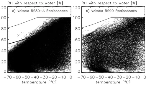
rate in the stratosphere. Miloshevich et al. (2001) showed a strong bias towards low humidity values at low temperatures for the Vaisala RS80-A radiosonde. He reported an underestimation in relative humidity of 1.3 at –35◦C, and 2.4 at –70◦C. Figure 1 de-picts the original RH measurements obtained at Ny- ˚Alesund by the different radioson-des. The data strongly suggests measured humidity values being far too low with the

10

RS80-A relative humidity measurements rarely reaching ice saturation at temperatures below –40◦C. But the existence of high supersaturation with respect to ice in the middle and upper troposphere is well documented (e.g., Ovarlez et al., 2002). When consid-ering data derived from the newer radiosondes RS90 and RS92, supersaturation with respect to ice is clearly reached much more often over the same range of ambient

15

temperatures. This underlines the need for a suitable data correction before further analysis. We used published algorithms to correct the available relative humidity data at Ny- ˚Alesund as stated out in the following paragraph. Parallel launched RS80-A and RS90 sondes allow us to validate the performed correction and to estimate a range within which we most probably expect the real relative humidity.

20

3.2 RH data correction procedure

Although the Vaisala RH sensors are all subject to the same general source of mea-surement errors, the magnitude of error depends strongly on the sensor type. Exper-iments have been performed to understand and quantify the source of RH measure-ment errors in RS80-A and RS90 sensors (Miloshevich et al., 2001, 2004, 2006; Wang

25

et al., 2002). These authors describe different sources of error for RH measurements 1266

(8)

ACPD

7, 1261–1293, 2007

Full Screen / Esc

and present empirically based methods to correct archived radiosonde data and quan-tify the importance of different errors in the data. We followed their approach to correct the three main types of errors presented in their papers, the contamination/calibration error, the temperature dependence, and the time lag effect.

First, the contamination error and two errors resulting from the sensor calibration

5

process are addressed. The basic RS80-A calibration model, more specifically the function relating capacitance to RH at a fixed temperature, has limitations. (Wang et al. 2002, hereinafter referred to as W02) proposed a correction equation (their Eq. 4.6-A) in the form of a fourth order polynomial to correct for this error. The contamination error was taken into account using W02 (their formula 4.1-A). As no information about

10

the age of an individual radiosonde was available, in this study we used a constant age of one year when calculating the age-dependence portion of the contamination correc-tion. Radiosondes are normally not stored more than one year at the station; therefore, our correction in this case will be on the upper limit. No contamination correction has been investigated for the RS90, because the error is thought to be much smaller due

15

to the replacement of Styrofoam in the radiosonde construction by cardboard (Miloshe-vich et al., 2004).

Second, the data were corrected for the temperature dependent error by applying for-mula 4.5 from W02. The temperature-dependent error is not a limitation of the sensor but is a consequence of the data processing algorithm. The temperature-dependent

20

coefficients delivered with the RS80-A describe a linear function of temperature, which is only an approximation to the actual non-linear temperature dependence of the sen-sor. The linear approximation leads to a temperature-dependent error that increases substantially with temperatures decreasing below –30◦C (Miloshevich et al., 2001).

Finally, the time lag error is corrected using the algorithm developed by Miloshevich

25

et al., (2004 hereinafter referred to as M04). At cold temperatures, the sensor is un-able to respond quickly to changes in the ambient RH, leading to a time-lag error that smoothes the RH profile and decreases the scale of details that are resolved. By using the sensor time constant as a function of temperature the vertical structure in the RH

(9)

ACPD

7, 1261–1293, 2007

Full Screen / Esc

profile, that is “smoothed” by the slow sensor response at cold temperatures, can be partly recovered.

The magnitude and sign of the correction varies according to the vertical humidity and temperature structure of a given profile, because it is sensitive to the local humidity gradient as well as to the temperature. RS90 data were also corrected for mean

cali-5

bration errors following the approach of (Miloshevich et al., 2006, hereinafter referred to as M06). The time lag, temperature dependence, and contamination corrections were combined and applied to the sounding data.

Furthermore, Miloshevich et al. (2001) presented a temperature dependent correc-tion factor derived from statistical analysis based on in-situ comparison of simultaneous

10

RH measurements from RS80-A radiosondes and the NOAA hygrometer. The formula used by (Miloshevich et al., 2001, hereinafter referred to as M01) is a fourth-order polynomial and was also applied to the RS80-A data.

3.3 Comparison analysis

The correction algorithms have been evaluated by comparing 12 RH profiles measured

15

simultaneously by RS80-A and RS90 sondes in March and April 2000. The RS80-A profiles were corrected using the published corrections W02 and M04 whereas RS90 profiles were corrected using M04 and M06 corrections. Furthermore, the statistical correction by M01 for the RS80-A profiles has also been tried and is also included in this analysis. We will use the corrected RS90 as reference for the performed comparison.

20

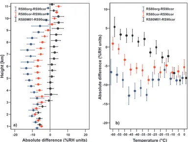
Figure 2 shows difference in relative humidity for the RS80-A and RS90 instruments as a function of altitude and temperature. The mean absolute difference between the RS80-A data and the corrected RS90 data can be as large as 15% (Fig. 2a). Figure 2b shows that the difference is generally larger at lower temperatures. After correcting for the contamination, time-lag and time dependent errors the mean RH difference is

sub-25

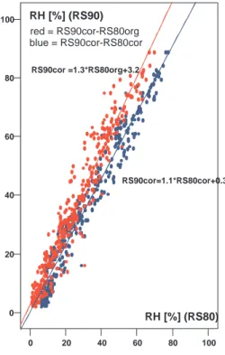
stantially reduced for temperatures above –50◦C (Fig. 2b). Figure 3 also illustrates the improved agreement between RS80-A and RS90 RH values for temperatures below –40◦C. Above –40◦C the influence of the correction is small. The statistical correction

(10)

ACPD

7, 1261–1293, 2007

Full Screen / Esc

using M01 for the RS80-A improves the difference for the temperature range between –10◦C to –40◦C but produces too high values at lower temperatures. The overall con-clusion from the analysis above is that the published corrections for the RS80-A allows us to estimate corrected RH typically within 10% of the newer RS90 radiosonde. The following analysis is based on 200 m averaged and corrected data.

5

4 Results and discussion

4.1 Mean relative humidity obtained from radiosonde data

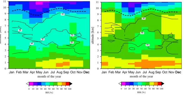
In this section, an overview is given of the statistical properties of the corrected RH data set. Figure 4 illustrates the corrected and monthly averaged RH and RHi (RH with respect to ice) values as a function of altitude. It also includes information where the

10

50% coefficient of variation (CV) is exceeded. The CV measures the relative scatter in data with respect to the mean and is a measure for the variance of the data. The higher the percentage the more variable the data distribution is. Below 2 km we found CV of less than 20% while the greatest variation is found at higher altitudes. The CV of 50% almost follows the mean tropopause height. There is also a region in

15

the free troposphere that is characterised by high variability from June to September. Below 2 km the RH measurements reached their maximum mean averaged values in summer of ∼90% RH compared to values of ∼70% RH in winter. However mean RHi shows much more vertical structure in the middle and upper troposphere compared to the mean RH and indicates a strong seasonal behaviour which encompasses a

20

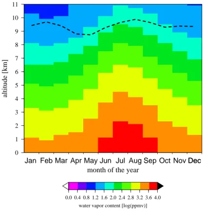
reduction of the mean RHi from winter of ∼80% to summer values of ∼60% RHi. Such a seasonal behaviour is also reported from analysed radiosondes and satellite data from Antarctica (Gettelman et al., 2006). In addition, Fig. 5 depicts the derived monthly mean water vapour content – as obtained by the radiosondes – as a function of altitude. There is a clear seasonal variation with higher mean water vapour contents in summer

25

than in winter. If we take, for example, a mean water vapour content in the altitude 1269

(11)

ACPD

7, 1261–1293, 2007

Full Screen / Esc

range from 2 to 8 km, the value in January is about 68% less than in July. 4.2 Frequency of ice supersaturation layers

Here we present the analysis of the occurrence of humid layers in the free troposphere where the RH reached supersaturation with respect to ice. These ice-supersaturation layers, where RH with respect to ice (RHi) is greater than 100%, are either potential

5

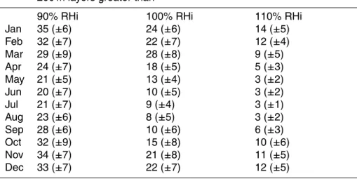
layers for both ice-supersaturated regions (clean air) or cirrus clouds. Based on the data averaging a layer corresponds to 200 m. Table 1 summarises the monthly mean frequency occurrence of such layers for RHi greater than 100% (±10%). The lower and upper limit take into account uncertainties in the measurements as described in Sect. 3.2. The standard deviation representing the inter-annual variation is also given

10

as an indicator of the variability within the data. As expected, the use of different RHi thresholds changes the frequency occurrence of ice-supersaturation layers but not the general temporal or spatial evolution. This gives us the confidence to restrict the further analysis to RHi layers greater than 100%. During the summer period (June– September), the occurrence is approximately half as frequent as during the rest of

15

the year. Ice-supersaturation is most frequent in winter (October–February; 22% of the data), less frequent in spring (March–May; 13%) and summer (June–September; 10%).

Overall, around 17% of all observations binned to 200 m layers are supersaturated with respect to ice (RHi>100%). More than 70% of the ascents showed more than

20

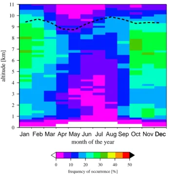
one layer where RHi >100%. In Fig. 6 we analysed the occurrence of these layers with respect to the month of the year and altitude. Based on the results of section 3.3, the range in uncertainty is typically ±10%. The frequency occurrence of the observed layers supersaturated with respect to ice at a certain altitude follows a clear annual cycle. Figure 6 demonstrates that saturation with respect to ice during fall/winter time

25

(October-February) is frequent in a broad upper tropospheric layer between ∼4 and 10 km. In summer (June-September), the layers saturated with respect to ice are less frequent and occur at higher altitudes generally between 7 and 9 km. A t-test was

(12)

ACPD

7, 1261–1293, 2007

Full Screen / Esc

highly significant at p =.000 for the seasonal shift. Figure 6 also indicates that the ice-supersaturation tends to consistently track the tropopause height. For temperatures below –35◦

C, about 47% of the layers supersaturated with respect to ice are within 1 km of the tropopause.

4.3 Comparison to other studies of radiosonde data

5

Observations from radiosondes suggest that the distribution of RHi in ice-supersaturated layers follows an almost exponential decay, indicating that the underly-ing processes, which cause this functional dependence, act in a statistically indepen-dent manner. This was reported in the analysis of humidity data from MOZAIC (Gierens et al., 1999), MLS (Spichtinger et al., 2002), radiosondes at Lindenberg (Spichtinger

10

et al., 2003), and TOVS data (Gierens et al., 2004). In the following we show that the Ny- ˚Alesund RHi data in excess of 100% also follow an exponential distribution for the upper troposphere. To make the results comparable to previous studies an alti-tude range above 4 km height was chosen. However, the features remain the same if we include the entire altitude range. In Fig. 6, we depict the (non-normalized)

fre-15

quency distributions of the relative humidity over ice N(RHi). Because the analysed layers saturated with respect to ice showed a strong seasonal behaviour (Fig. 6) the frequency distributions were determined for different seasons (fall/winter =October-February, spring=March–May and summer=June–September). The single RHi values are binned into 150 1% wide classes (numbered from 0–149), where the last class

20

(149) contains all data with RHi ≥149%.

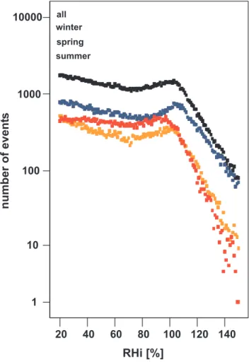
The seasonal curves show similar behaviour. Each curve is relatively smooth below 100% RHi but reach a small maximum near 100%. Above 100%, the frequency occur-rence of ice-supersaturation levels decreases exponentially in all seasons. The steep-ness of the exponential curve and location of the maximum show significant seasonal

25

dependence (Fig. 7). Gierens et al.,(2004) interpreted the existence of the local maxi-mum, or bulge, around 100% RHi to be a product of cloud processes. All distributions follow the same structure, approximately uniform below ice saturation and decreasing

(13)

ACPD

7, 1261–1293, 2007

Full Screen / Esc

geometrically above. The exponents b=-ln q for distributions RHi have been computed for the range 20%≤ RHi ≤80% and 110%≤ RHi ≤150%, respectively, using a straight line fit to the function ln(N(k))= a-b*k (see Table 2 for the obtained results). For the supersaturated range the exponents range from 0.057 in fall/winter to 0.11 in summer. The result of the previous subsection can be used to infer the mean ice-supersaturation

5

knowing that the expected value of a modified geometric distribution is q/(1-q) = e−b /(1-e−b), therewith the mean ice-supersaturation above 4 km altitude amounts to 15% on average, with seasonal variations in winter of 17%, in spring of 12% and summer of 8%, whereas ice nucleation requires 30% supersaturation on the average (Gierens et al., 1999). More resent studies indicate that homogeneous freezing affords even higher

10

supersaturation around 145% (e.g. Haag et al., 2003).

These results may be compared with those of Spichtinger et al., (2003), who applied a similar analysis to one year’s radiosonde data from Lindenberg, and observed a much steeper exponent value of 0.21. Also relevant for the present study are results of Gierens et al. (1999), based on three years of data obtained from MOSAIC (b=0.058),

15

and from Spichtinger et al. (2002) who obtained b=0.051 from MSL data. As they do not separate data into seasons, our value for the entire data set above 4 km altitude of b = 0.066 compares to their results. However, their results are averaged over large geo-graphical regions and are not immediately comparable with a single isolated station, as Ny- ˚Alesund. We note that the summer distribution is different than the other seasons.

20

A similar seasonal pattern in RHi distribution was reported by Vaughan et al. (2005) for mid-latitude upper tropospheric radiosonde data from Wales. The local maximum of the summer distribution (red dots) is located just below ice saturation, whereas the spring maximum (orange dots) is almost right at and winter maximum (blue dots) is above ice saturation (Fig. 7). We also note that the observed bulge is less pronounced

25

in summer compared to the other periods. The total frequency of RHi layers greater than 100% is only about 5% during the summer compared to 18% for the rest of the year. It is possible that dynamic processes suppress the build-up of high supersatu-ration in summer or that differences in cloud processes create the observed seasonal

(14)

ACPD

7, 1261–1293, 2007

Full Screen / Esc

differences.

Besides RH analysis, we also calculated the mean temperature and 98% percentile values, in ice-supersaturated layers and non ice-supersaturated layers (see Table 2). Depending on the season, the mean temperature behaviour is different for both layer types. Mean temperatures in ice-supersaturated layers tend to be lower (2 K) than

5

in non supersaturated layers only in summer whereas during winter/fall, the ice-supersaturated layers are about 5 K warmer than the non ice-ice-supersaturated layers. We currently do not have an explanation for this difference. The colder air in supersaturated layers suggests that uplifting of airmasses is one major source of ice-supersaturation layers as discussed by Gierens et al. (1999) in connection to MOZAIC

10

data. The flight data is different from the radiosonde data as aircraft measurements are made on a specific pressure level and the sounding data provides information in the vertical. Another possible origin of ice-supersaturation in the troposphere might be advection of moisture leading to variations in absolute water vapour content. We have determined mean and standard deviation of the water vapour content. The

re-15

sults are displayed in Table 3. The standard deviations are comparable, or larger than the mean values. The derived mean values show that water vapour content is con-siderable larger in ice-supersaturation layers than in non ice-supersaturation layers. The lowest values of water vapour content for supersaturation layers and non ice-supersaturation layers are reached in winter/fall. The ratio between the two layer types

20

is highest in winter/fall with 2.9 and lowest in summer with 2.1. The general evolution of the water vapour content in the Arctic atmosphere over Ny- ˚Alesund can also be seen in Fig. 5. Therefore, we believe that moisture advection plays an important role in the formation of ice-supersaturated regions.

4.4 Vertical and seasonal variation extent of ice-supersaturation layers

25

The profiles of RH measurements allow us to investigate the vertical extent of the ice-supersaturation layers. Of special interest is the cloud’s ability to reflect sunlight and thus influence the radiative balance and this depends on the cloud’s thickness.

(15)

ACPD

7, 1261–1293, 2007

Full Screen / Esc

Spichtinger et al. (2004) discussed the differences in the bulge signature in frequency distributions of the relative humidity over ice as possibly related to different cloud thick-ness. To be able to compare our results to Spichtinger et al. (2004), we restrict our data base to layers above 4 km height.

In order to derive the vertical extent of ice-supersaturation for each single sounding

5

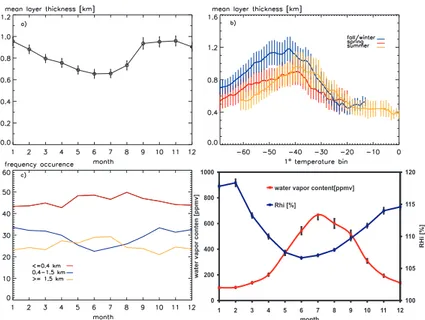
profile, we combined all adjacent 200 m ice-supersaturation layers into one single layer. Each such layer is then characterised by the altitude of its lower and upper boundary, its depth (layer thickness) as well as its mid-layer temperature. The mean layer thickness reaches its minimum of ∼0.7 km in summer (Fig. 8a) increasing by ∼50% in winter. Figure 8b shows the mean layer thickness as a function of mid layer temperature and

10

season. Figure 8b shows the mean layer thickness as a function of mid layer tem-perature and season. For the different seasons, the principal shape of the curve is very similar and the maximum layer thickness is in all cases reached at temperatures around –40◦C. Indeed, approximately 54% of the adjacent ice-supersaturated layers have a mid-layer temperature that below -35◦

C. As Lidar measurements by Goldfarb et

15

al. (2001) in France and Cadet et al. (2003) in Reunion determined an average cloud layer thickness for cirrus of approximately 1.4 km ±1.3 and a markedly thinner cloud layer thickness for subvisible clouds between 0.4 and 0.8 km we were interested in how the thickness of the ice-supersaturation layers develops from month to month in our case. To do this we divided the layer thickness in different ranges as depicted in

20

Fig. 8c. One interesting difference is the increase of thin layers with a thickness of up to 40 m and layers thicker than 1.5 km in summer when a minimum of layers between 0.4 and 1.5 km was observed. With our actual data set we are not able to determine what causes these seasonal differences. Fig. 8d demonstrates the evolution of the monthly averaged RHi obtained in the ice-supersaturation layers and of the corresponding

wa-25

ter vapour content. The shape of the both curves highly suggests an anticorrelation between the both values.

A method to get more detailed information on the vertical extent of these layers was described by Spichtinger et al., (2003). Using a statistical approach described by

(16)

ACPD

7, 1261–1293, 2007

Full Screen / Esc

Berton (2000) to analyse ice-supersaturation layers they showed that the thickness of ice-supersaturation layers over Lindenberg followed a Weibull distribution, with different slopes for shallow and thicker layers, and determined that the transition between the two regimes occurred around 1km thickness. We performed the same analysis for our data set and found the transition occurred at a thickness around 2 km. The data points

5

referring to deeper layers are most likely taken inside cirrus clouds. The slope of the line in this part is 0.9. For visible cirrus, the corresponding shape parameter is around 1 (Berton, 2000; Spichtinger et al., 2003). Layers less thick than 2 km probably contain data from true ice-supersaturation layers and perhaps sub-visible cirrus. The slope for these thinner layers is around 0.5. Almost 90% of the layers are thinner than 2 km.

10

As not only layer thickness but also the available cloud water content is important for determining cloud characteristics this can only act as a first step in the analysis of the ice-supersaturation layers. This needs further investigation especially coupling the RHi data with remote sensing data obtained from Ny- ˚Alesund such as micropulse Lidar or ceilometer in order to get more insight in the layer characteristics.

15

4.5 Combining ice-supersaturation layers and subvisible clouds detected by SAGE II We further studied the relation between ice-supersaturated layers and subvisible clouds (SVC) by looking at data from the Stratospheric Aerosol and Gas Experiment II (SAGE II) satellite. Gierens et al. (2000) showed an association between ice-saturated regions with SAGE II SVC. SAGE II aerosol products open up the possibility to

inves-20

tigate the occurrence of SVC in the Arctic on a statistical basis. Ideally one would like to correlate the occurrence of SVC and the existence of ice-supersaturation on a case by case basis. Unfortunately this is not practicable with the SAGE data. Single events cannot be used here because it is rather rare that SAGE measurements and the radio sonde soundings are collocated in time. Thus, we decided to compare the data on a

25

monthly basis for all data available North of 60◦and averaged the sounding results to the height grid of SAGE II. The approach of analysing monthly averaged SAGE data was already used to derive principal aerosol characteristics in the upper Arctic

(17)

ACPD

7, 1261–1293, 2007

Full Screen / Esc

sphere (Treffeisen et al., 2006). The SVC from SAGE II are most often detected around the tropopause height. Approximately 80% of the detected SVC are located within 3 km of the tropopause. The vertical distribution of SVC detected by SAGE is presented for the spring and summer period in Fig. 9, together with the frequency of occurrence of ice-supersaturated layers. The peak of occurrence of SVC is well pronounced in

5

both periods showing a maximum of about 24% in March to April compared to 15% in summer whereas the location of the maximum is shifted only slightly from 8.5 km in spring to 9 km in summer for the SAGE II measurements. The general similarity between the altitude distributions is very good. Where the frequency occurrence ice-supersaturation is high, the occurrence of SVC is also high, and visa versa. Restricting

10

ice-supersaturation layers to temperatures below –40◦C increases the agreement for the lower altitude ranges. Based on these results, the largest part of the observed ice-supersaturation layers is most probably representing subvisible clouds. A statistical analysis of cloud occurrence performed on 11 month of data from Ny- ˚Alesund showed 5% of clouds to be in the altitude range from 6 to 12 km on average and thicker clouds

15

in summer than in winter time (Shiobara et. al, 2003). Future studies should directly compare cloud measurements with the obtained ice-supersaturation layers.

Considering the large temporal and vertical variability, the agreement between SAGE II SVC and ice-supersaturated layers from radiosondes is very good. The differences in location and height of the maximum in spring (Fig. 9) might be due to processes

20

that decouple SVC from ice-supersaturation layers and ice-supersaturation alone does not produce a unique spectral signature in the SAGE II data. Differences can also result from the large spatial coverage of the SAGE II satellite, compared to the point measurement with the radiosonde, and the quality of the SAGE II cloud measurements which can affected by aerosol-cloud mixture, fractional cloud coverage of the viewing

25

window and fractional cloud distribution along the viewing window and viewing path (Wang et al., 1995).

(18)

ACPD

7, 1261–1293, 2007

Full Screen / Esc

5 Conclusions

We analysed a unique high latitude data set of tropospheric humidity profiles mea-sured with standard radiosondes at Ny- ˚Alesund (78◦55′N 11◦52′E) during the period from 1991 to 2005. The sounding data were corrected using previously published al-gorithms. Despite the extensive corrections, there is still an uncertainty associated

5

with the difficulties of radiosonde RH measurements in cold temperatures and we were not able to lower the realistic error below ±10% RH. The corrected data were used to determine main characteristics of the tropospheric relative humidity distribution in the vicinity of Ny- ˚Alesund. It is clear from the radiosondes that supersaturation with respect to ice is observed throughout the year. It indicates that supersaturation over

10

ice is a frequent condition in the Arctic middle and upper troposphere, particularly dur-ing fall/winter. The frequency occurrence of ice-supersaturation levels decreases ex-ponentially with the magnitude of ice-supersaturation and is in good agreement with other studies. The mean frequency occurrence of ice-supersaturation layers above 4 km follows a clear seasonal variation with a value of 17% in winter, 12% in spring

15

and 8% in summer. The ice-supersaturation occurs mostly in a broad band between 6 and 9 km in winter and undergoes a shifting towards higher altitudes in summer. The altitude distribution of ice-supersatured layers over Ny- ˚Alesund is generally similar to that of subvisible clouds from the SAGE II experiment and thus confirms the existence of SVC in the Arctic atmosphere. While one might expect the soundings to observe

20

different frequencies than SAGE II, owing to the different sampling volumes (the SAGE II instrument samples horizontal distances of ∼200 km), our results show that there is a strong positive correlation between both independent observations, which indicates that ice-supersaturated layers associated with sub-visible cirrus are likely to be a wide spread phenomenon over the Arctic. This brings attention to the important issue of the

25

SVC influence on the radiative budget in the Arctic, which is currently unexplored. This study focused on a general first description of the ice-supersaturation layers over Ny- ˚Alesund. Continuation of this work will attempt to compare these presented

(19)

ACPD

7, 1261–1293, 2007

Full Screen / Esc

results directly to ground-based Lidar systems and CALIPSO satellite data. This can give us information on the internal structure of the layers and will help us to understand cloud formation processes

Acknowledgements. We give thanks to the following: For financial support to International

Me-teorological Institute (IMI), Swedish Research Council, Swedish Polar Secretariat and Alfred

5

Wegener Institute, who made this study possible.

References

Baker, M. B.: Cloud microphysics and climate, Science, 276, 1072–1078, 1997.

Bakan, S., Betancor, M., Gayler, V., and Grassl, H.: Contrail frequency over Europe from NOAA satellite images, Ann. Geophys., 12, 962–968, 1994,

10

http://www.ann-geophys.net/12/962/1994/.

Bates, J. J., and Jackson, D. J.: Trends in upper-tropospheric humidity, Geophys. Res. Lett., 28, 1695, 2001.

Berton, R. P. H.: Statistical distribution of water content and sizes for clouds above Europe, Ann. Geophys., 18, 385–397, 2000,

15

Cadet, B., Goldfarb, L., Faduilhe, D., Baldy, S., Giraud, V., Keckhut, P., and R ´echou, A.: A sub-tropical cirrus clouds climatology from Reunion Island (21◦

S, 55◦

E) lidar data set, Geophys. Res. Lett., 30, 10.1029/2002GL016342, 2003.

Elliott, W. P. and Gaffen, D. J.: On the utility of radiosonde humidity archives for climate studies.

20

Bull. Amer. Meteor. Soc., 72, 1507–1520, 1991.

Gettelman, A., Walden, V. P., Miloshevich, L. M., Roth, W. L., and Halter, B.: Relative humidity over Antarctica from radiosondes, satellites, and a general circulation model, J. Geophys. Res., 111, D09S13, doi:10.1029/2005JD006636, 2006.

Gierens, K, Schumann, U., Helten, M., Smit, H., and Marenco, A.: A distribution law for

rel-25

ative humidity in the upper troposphere and lower stratosphere derived from three years of MOZAIC measurements, Ann. Geophys., 17, 1218–1226, 1999,

Gierens, K., Schumann, U., Helten, M., Smit, H., and Wang, P.-H.: Ice-supersaturated

(20)

ACPD

7, 1261–1293, 2007

Full Screen / Esc

gions and subvisible cirrus in the northern midlatitude upper troposphere, J. Geophys. Res., 105(D18), 22 743–22 754, doi:10.1029/2000JD900341, 2000.

Gierens, K., Kohlhepp, R., Spichtinger, P., and Schroedter-Homscheidt, M.: Ice supersaturation as seen from TOVS, Atmos. Chem. Phys., 4, 539–547, 2004,

http://www.atmos-chem-phys.net/4/539/2004/.

5

Goldfarb, L., Keckhut, P., Chanin, M.-L., and Hauchecorne, A.: Cirrus Climatological Re-sults from Lidar Measurements at OHP (44◦N, 6◦E), Geophys. Res. Lett., 28, 1687–1690, doi:10.1029/2000GL012701, 2001.

Haag, W., K ¨archer, B., Str ¨om, J., Minikin, A., Lohmann, U., Ovarlez, J., and Stohl, A.: Freezing thresholds and cirrus cloud formation mechanisms inferred from in situ measurements of

10

relative humidity, Atmos. Chem. Phys., 3, 1791–1806, 2003,

Kent, G. S., Winkler, D. M., Osborn, M. T., and Skeens, K. M.: A model for the separation of cloud and aerosol in SAGE II occultation data, J. Geophys. Res., 98, 20 725–20 735, 1993. Koop, T., Puo, B.L., Tsias, A., and Peter, T.: Water activity as the determinant for homogeneous

15

ice nucleation in aqueous solutions, Nature, 406, 611–614, 2000.

Liou, K.-N.: Influence of cirrus clouds on weather and climate processes: A global perspective, Mon. Weather Rev., 114, 1167–1199, 1986.

Miloshevich, L. M., V ¨omel, H., Paukkunen, A., Heymsfield, A. J., and Oltmans, S. J.: Character-ization and Correction of Relative Humidity Measurements from Vaisala RS80-A

Radioson-20

des at Cold Temperatures, J. Atmos. Oceanic Technol., 18, 135–156, 2001.

Miloshevich, M., Paukkunen, A., V ¨omel, H., and Oltmans, S.: Development and Validation of a Time-Lag Correction for Vaisala Radiosonde Humidity Measurements, J. Atmos. Oceanic Technol., 21, 1305–1327, 2004.

Miloshevich, L. M., V ¨omel, H., Whiteman, D. N., Lesht, B. M., Schmidlin, F. J., and Russo,

25

F.: Absolute accuracy of water vapor measurements from six operational radiosonde types launched during AWEX-G and implications for AIRS validation, J. Geophys. Res., 111, D09S10, doi:10.1029/2005JD006083, 2006.

Murphy, D. M., Kelly, K. K., Tuck, A. F., Proffitt, M. H., and Kinne, S.: Ice satu-ration at the tropopause observed from the ER-2 aircraft. Geophys. Res. Lett., 17,

30

doi:10.1029/90GL00327, 1990.

Ovarlez, J., Gayet, J. F., Gierens, K., Str ¨om, J., Ovarlez, H., Auriol, F., Busen, R., and Schu-mann, U.: Water vapour measurements inside cirrus clouds in Northern and Southern

(21)

ACPD

7, 1261–1293, 2007

Full Screen / Esc

spheres during INCA, Geophys. Res. Lett., 29, 16, doi:10.10298/2001GL014440, 2002. Randel, D. L., Vonder Haar, T. H., Ringerud, M. A., Stephens, G. L., Greenwald, T. J., and

Combs, C. L.: A New Global Water Vapor Dataset. Bull. Amer. Meteor. Soc., 77, 1233–1246, 1996.

Schmidlin, F. J., and Ivanov, A.: Radiosonde relative humidity sensor performance: The WMO

5

intercomparison–Sept 1995. Preprints, 10th Symp. on Meteorological Observations and In-strumentation, Phoenix, AZ, Amer. Meteor. Soc., 68–71, 1998.

Stephens, G. L., Tsay, S. C., Stackhouse, P. W., and Flatau, P. J.: The relevance of the micro-physical and radiative properties of cirrus clouds to climate and climatic feedback, J. Atmos. Sci., 47, 1742–1753, 1990.

10

Shiobara, M., Yabuki, M., and Kobayashi, H.: A polar cloud analysis based on Micor-pulse Lidar measurements at Ny- ˚Alesund, Svalbard and Syowa, Antarctica, Phys. Chem. Earth, 28, 1205–1212, 2003.

Spichtinger, P., Gierens, K., and Read, W.: The statistical distribution law of relative humidity in the global tropopause region, Meteorol. Z., 11, 83–88, 2002.

15

Spichtinger, P., Gierens, K., Leiterer, U., and Dier, H.: Ice supersaturation in the tropopause region over Lindenberg, Germany, Meteorol. Z., 22, 143–156, 2003.

Treffeisen, R. E., Thomason, L. W., Str ¨om, J., Herber, A. B., Burton, S. P., and Yamanouchi, T.: SAGE II and III aerosol extinction measurements in the Arctic middle and upper troposphere., J. Geophys. Res. 111, D17203, doi:10.1029/2005JD006271, 2006.

20

Vaughan, G., Cambridge, C., Dean, L., and Phillips, A. W.: Water vapour and ozone profiles in the midlatitude upper troposphere, Atmos. Chem. Phys., 5, 963–971, 2005,

Wang, P. H., Mc Cormick, M. P., Poole, L. R., Chu, W. P., Yue, G. K., Kent, G. S., and Skeens, K. M.: Tropical high cloud characteristics derived from SAGE II extinction measurements,

25

Atmos. Res., 34, 53–83, 1994.

Wang, P. H., Minnis, P., and Yue, G. K.: Extinction coefficient (1 µm) properties of high altitude clouds from solar occultation measurements (1985–1990): evidence of volcanic aerosol ef-fect, J. Geophys. Res., 100 (2), 3181–3199, 1995.

Wang, P.-H., Minnis, P., McCormick, M. P., Kent, G. S., and Skeens, K. M.: A 6-year climatology

30

of cloud occurrence frequency from Stratospheric Aerosol and Gas Experiment II observa-tions (1985–1990), J. Geophys. Res., 101, 29 407–29 429, 1996.

Wang, J., Cole, H., Carlson, L., , Miller, D.J., , Beierle, E.R., Paukkunen, K., and Laine, T.K.:

(22)

ACPD

7, 1261–1293, 2007

Full Screen / Esc

Corrections of Humidity Measurement Errors from the Vaisala RS80 Radiosonde-Application to TOGA COARE Data, J. Atmos. Oceanic Technol., 19, 981–1002, 2002.

WMO: Measurements of upper air temperature, pressure, and humidity. Guide to Meteorologi-cal Instruments and Methods of Observation, 6th ed., WMO I.12–1–I.12–32, 1996.

Wylie, D. P., Menzel, W. P., Woolf, H. M., and Strabala, K.: Four Years of Global Cirrus Cloud

5

Statistics Using HIRS, J. Clim., 7, 1972–1986, 1994.

(23)

ACPD

7, 1261–1293, 2007

Full Screen / Esc

Printer-friendly Version Interactive Discussion Table 1. Monthly mean frequency occurrence of ice-supersaturation layers for different RHi

thresholds. Profiles analysed up to 11 km height. Standard deviation represents the inter-annual variation within the 14 years analysed.

200 m layers greater than

90% RHi 100% RHi 110% RHi Jan 35 (±6) 24 (±6) 14 (±5) Feb 32 (±7) 22 (±7) 12 (±4) Mar 29 (±9) 28 (±8) 9 (±5) Apr 24 (±7) 18 (±5) 5 (±3) May 21 (±5) 13 (±4) 3 (±2) Jun 20 (±7) 10 (±5) 3 (±2) Jul 21 (±7) 9 (±4) 3 (±1) Aug 23 (±6) 8 (±5) 3 (±2) Sep 28 (±6) 10 (±6) 6 (±3) Oct 32 (±9) 15 (±8) 10 (±6) Nov 34 (±7) 21 (±8) 11 (±5) Dec 33 (±7) 22 (±7) 12 (±5) 1282

(24)

ACPD

7, 1261–1293, 2007

Full Screen / Esc

Printer-friendly Version Interactive Discussion Table 2. Exponents b for the frequency distribution law ln[N(k)] = a–b*k as obtained from

straight fitting to the distribution of relative humidity with respect to ice, RHi, shown in Fig. 4. The standard deviation σb for the determined values b is given in brackets. Values have

been multiplied by 100 for easier reading. Mean and 98% percentile of temperature for ice-supersaturation layers (ISS) and non ice-ice-supersaturation layers (Non-ISS). All values above 4 km height up to 2 km above tropopause height. All data averaged on 200 m steps. Fall/winter (October–February); spring (March–May) and summer (June–September).

Fit range Temperature [◦C] Non–ISS ISS 110–150 20–80 mean 98% mean 98% Total 6.6 (0.1) 0.8 (0.0) –52.3 (16) –18.9 –50.0 (14) –22.9 Fall/Winter 5.7 (0.1) 0.9 (0.0) –58.3 (14) –27.0 –53.0 (14) –26.2 Spring 7.9 (0.2) 1.1 (0.1) –51.0 (13) –24.1 –48.9 (13) –25.5 Summer 11.2 (0.6) 0.4 (0.0) –38.5 (12) –13.5 –40.5 (12) –17.4 1283

(25)

ACPD

7, 1261–1293, 2007

Full Screen / Esc

Printer-friendly Version Interactive Discussion Table 3. Mean and 98% percentile of ppmv for ice-supersaturation layers (ISS) and for non

ice-supersaturation layers (Non – ISS). All values above 4 km height data averaged on 200 m steps. Fall/winter (October–February); spring (March–May) and summer (June–September).

Water vapour content [ppmv] Non–ISS ISS

ratio mean 98% mean 98% Total 1.9 153 (337) 1283 287 (409) 1593 Fall/Winter 2.9 72 (164) 574 209 (294) 1142 Spring 2.1 121 (216) 826 259 (297) 1175 Summer 1.5 391 (575) 2270 590 (653) 2548

(26)

ACPD

7, 1261–1293, 2007

Full Screen / Esc

Fig. 1. Data set of RH measurements from Ny- ˚Alesund radiosondes. (a) for RS80 radiosondes

between mid October 1991 and mid July 2002 (b) for RS90/RS92 radiosondes between mid July 2002 and December 2005. All data points are averaged over 200 m and restricted to values below 2 km above the tropopause height (WMO, 1996). Thick solid curve is ice saturation and light solid line is the homogenous ice nucleation level from Koop et al. (2000).

(27)

ACPD

7, 1261–1293, 2007

Full Screen / Esc

Printer-friendly Version Interactive Discussion 1 2 3 4 5 6 7 8 9 10 11 Height [km] -20 -10 0 10 20

Absolute difference (%RH units) a) -60 -55 -50 -45 -40 -35 -30 -25 -20 -15 -10 -5 0 Temperature (°C) -20 -15 -10 -5 0 5 10 Absolute difference (%RH unit s) b)

Fig. 2. Absolute humidity difference between corresponding RS80-A and RS90 measurements

shown as function of height (a) and temperature (b) for 12 tandem flights in March and April 2000. Data points are the mean in 500 m height bins or 5◦

C temperature bins including the 95% confidence interval of the mean. Plotted are the difference between the original RS80-A data and corrected RS90 data as described in Sect. 3.2 (blue), the difference between the corrected RS80-A and RS90 data (red) as well as the difference between the RS80-A using the approach of M01 and RS90 corrected (black).

(28)

ACPD

7, 1261–1293, 2007

Full Screen / Esc

Printer-friendly Version Interactive Discussion 0 20 40 60 80 100 0 20 40 60 80 100 RH [%] (RS90) RH [%] (RS80) red = RS90cor-RS80org blue = RS90cor-RS80cor RS90cor =1.3*RS80org+3.2 RS90cor=1.1*RS80cor+0.3

Fig. 3. Correlation RS80-A and RS90 for temperatures below –40◦

C before and after correction as described in Sect. 3.2 for the 12 tandem flights performed in March and April 2000 at

Ny-˚

Alesund.

(29)

ACPD

7, 1261–1293, 2007

Full Screen / Esc

Printer-friendly Version Interactive Discussion 0 1 2 3 4 5 6 7 8 9 10 11 altitude [km]

month of the year

50 50 50 50 50 50 50 50 50 50 50 50

Jan Feb Mar Apr May Jun Jul Aug Sep Oct Nov DecDec

0 10 20 30 40 50 60 70 80 90 100 RH [%] 0 1 2 3 4 5 6 7 8 9 10 11 altitude [km]

month of the year

50 50 50 50 50 50

0 10 20 30 40 50 60 70 80 90 100

RHi [%]

Fig. 4. Monthly mean of RH (left panel) and RHi (right panel). Also plotted with black solid lines

where the 50% coefficient of variation (CV) is exceeded. Dashed line represents the mean tropopause height determined using the WMO’s definition of the tropopause (WMO, 1996).

(30)

ACPD

7, 1261–1293, 2007

Full Screen / Esc

month of the year

0.0 0.4 0.8 1.2 1.6 2.0 2.4 2.8 3.2 3.6 4.0 water vapor content [log(ppmv)]

Fig. 5. Monthly mean of water vapour content. Dashed line represents the mean tropopause

height. Dashed line represents the mean tropopause height determined using the WMO’s definition of the tropopause (WMO, 1996).

(31)

ACPD

7, 1261–1293, 2007

Full Screen / Esc

month of the year

0 10 20 30 40 50

frequency of occurrence [%]

Fig. 6. Monthly mean frequencies occurrence of ice-supersaturation layers. The frequency of

occurrence are defined here as the number of observations in an 200 m altitude range where RH with respect to ice is greater than 100% divided by the total number of observations for this altitude range. Dashed line represents the mean tropopause height determined using the WMO’s definition of the tropopause (WMO, 1996).

(32)

ACPD

7, 1261–1293, 2007

Full Screen / Esc

Printer-friendly Version Interactive Discussion 20 40 60 80 100 120 140 RHi [%] 1 10 100 1000 10000 number of event s winter spring summer all

Fig. 7. Frequency distribution (per 1% RHi bins) of relative humidity with respect to ice (RHi),

for data above 4 km height (all; black); including seasonal frequency distribution for fall/winter (October–February; blue), spring (March–May; orange) and summer (June–September; red).

(33)

ACPD

7, 1261–1293, 2007

Full Screen / Esc

Printer-friendly Version Interactive Discussion 0 200 400 600 800 1000 1 2 3 4 5 6 7 8 9 10 11 12 month w a ter vapor conten [ppmv] 100 105 110 115 120 RHi [% ]

water vapor content[ppmv] Rhi [%]

Fig. 8. This figures show different statistics on all determined adjacent supersaturation layers

above 4 km height: (a) Monthly mean of the amount of the layer thickness and the standard de-viation of the mean; (b) mean layer thickness and standard dede-viation of the mean as a function of 1◦

temperature bins based on the mid-layer temperature for different seasons; values are averaged with a 10◦ moving average; fall/winter (October–February), spring (March–May) and summer (June–September); (c) monthly occurrence of different thickness ranges; (d) Monthly averaged water vapour content (red line) and RHi of adjacent ice- supersaturation layers.

(34)

ACPD

7, 1261–1293, 2007

Full Screen / Esc

Printer-friendly Version Interactive Discussion Fig. 9. Mean frequency distribution of all ice-supersaturation layers obtained by the

radioson-des (red line) and ice-supersaturation layers when the temperature is below –40◦C (green line). As well depicted the frequency of occurrence of SVC vs. altitude, as obtained from SAGE II satellite measurements for the latitude band 60◦

N–80◦

N; (a) calculated for March, April and May; (b) calculated for June, July, August and September.