Advanced spectral methods for climatic time series

HAL Id: hal-03222744

https://hal.archives-ouvertes.fr/hal-03222744

HAL is a multi-disciplinary open access archive for the deposit and dissemination of sci-entific research documents, whether they are pub-lished or not. The documents may come from teaching and research institutions in France or abroad, or from public or private research centers.

L’archive ouverte pluridisciplinaire HAL, est destinée au dépôt et à la diffusion de documents scientifiques de niveau recherche, publiés ou non, émanant des établissements d’enseignement et de recherche français ou étrangers, des laboratoires publics ou privés.

Advanced spectral methods for climatic time series

M. Ghil, M. R. Allen, M. D. Dettinger, K. Ide, D. Kondrashov, M. E. Mann,

A. W. Robertson, A. Saunders, Y. Tian, F. Varadi, et al.

To cite this version:

M. Ghil, M. R. Allen, M. D. Dettinger, K. Ide, D. Kondrashov, et al.. Advanced spectral methods for climatic time series. Reviews of Geophysics, American Geophysical Union, 2002, 40 (1), pp.3. �10.1029/2000rg000092�. �hal-03222744�

TIME SERIES

M. Ghil,1,2_{M. R. Allen,}3 _{M. D. Dettinger,}4_{K. Ide,}1

D. Kondrashov,1_{M. E. Mann,}5 _{A. W. Robertson,}1,6

A. Saunders,1_{Y. Tian,}1,7_{F. Varadi,}1_{and P. Yiou}8

Received 28 August 2000; revised 3 July 2001; accepted 18 September 2001; published 13 September 2002.

[1] The analysis of univariate or multivariate time series

provides crucial information to describe, understand, and predict climatic variability. The discovery and im-plementation of a number of novel methods for extract-ing useful information from time series has recently revitalized this classical field of study. Considerable progress has also been made in interpreting the infor-mation so obtained in terms of dynamical systems the-ory. In this review we describe the connections between time series analysis and nonlinear dynamics, discuss sig-nal-to-noise enhancement, and present some of the novel methods for spectral analysis. The various steps, as well as the advantages and disadvantages of these meth-ods, are illustrated by their application to an important

climatic time series, the Southern Oscillation Index. This index captures major features of interannual climate vari-ability and is used extensively in its prediction. Regional and global sea surface temperature data sets are used to illustrate multivariate spectral methods. Open questions and further prospects conclude the review.INDEXTERMS: 1620

Climate dynamics (3309); 3220 Nonlinear dynamics; 4522 El Nin˜o; 9820 Techniques applicable in three or more fields; KEYWORDS:

cli-mate; dynamical systems; El Nin˜o; prediction; spectral analysis; time series

Citation:M. Ghil, M. R. Allen, M. D. Dettinger, K. Ide, D. Kondra-shov, M. E. Mann, A. W. Robertson, A. Saunders, Y. Tian, F. Varadi, and P. Yiou, Advanced spectral methods for climatic time series, Rev. Geophys., 40(1), 1003, doi:10.1029/2000RG000092, 2002.

CONTENTS

1. Introduction and Motivation . . . 1

1.1. Analysis in the time domain versus the spectral domain . . . 3

1.2. Time series and nonlinear dynamics . . . . 4

2. Enhancing the Signal-to-Noise (S/N) Ratio . . . 6

2.1. Motivation for singular spectrum analysis (SSA) . . . 6

2.2. Decomposition and reconstruction . . . 7

2.3. Monte Carlo SSA . . . 11

2.4. Multiscale SSA and wavelet analysis . . . . 13

3. Spectral Analysis Methods . . . 16

3.1. Generalities and definitions . . . 16

3.2. Classical spectral estimates . . . 17

3.3. Maximum entropy method (MEM) . . . 18

3.4. Multitaper method (MTM) . . . 20

4. Multivariate Methods . . . 25

4.1. Principal oscillation patterns (POPs) . . . . 26

4.2. Multichannel SSA (M-SSA) . . . 26

5. Summary and Perspectives . . . 30

5.1. Summary . . . 30

5.2. Implications for understanding . . . 32

5.3. Implications for prediction . . . 33

Appendix A: SSA, Spatial EOFs, and the Karhu-nen-Loe`ve Theorems . . . 34

A1. Spatial and temporal EOFs . . . 34

A2. Complementary windows for M-SSA . . . . 35

1. INTRODUCTION AND MOTIVATION

[2] A time series provides useful information about

the physical, biological, or socioeconomic system that produced it. The purpose of time series analysis is to determine some of the system’s key properties by quan-1_{Department of Atmospheric Sciences and Institute of}

Geophysics and Planetary Physics, University of California, Los Angeles, Los Angeles, California, USA.

2_{Also at De´partement Terre-Atmosphe`re-Oce´an and}

Labo-ratoire de Me´te´orologie Dynamique, Ecole Normale Su-pe´rieure, Paris, France.

3_{Space Science and Technology Department, Rutherford}

Appleton Laboratory, Chilton, Didcot, England.

4_{U.S. Geological Survey, San Diego, California, USA.} 5_{Department of Environmental Sciences, University of}

Vir-ginia, Charlottesville, VirVir-ginia, USA.

6_{Now at International Research Institute for Climate}

Pre-diction (IRI), Palisades, New York, USA.

7_{Now at NASA Goddard Space Flight Center, Greenbelt,}

Maryland, USA.

8_{Laboratoire des Sciences du Climat et de l’Environnement,}

UMR CEA-CNRS, Gif-sur-Yvette, France.

Copyright 2002 by the American Geophysical Union. Reviews of Geophysics, 40, 1 / March 2002 8755-1209/02/2000RG000092 1003, doi:10.1029/2000RG000092

TABLE 1. Glossary of the Principal Symbolsa

Symbol Definition Method Section

Ak(t) kth principal component (PC) of {X(t)} SSA 2.2

Akb(t) kth local PC of {X(t)} at time b SSA 2.4

A(t), An continuous- and discrete-time envelope function MTM 3.4

Ak _{kth multichannel PC SSA 4.2}

a dilation factor of␺(x) 3 ␺(x/a) WLTs 2.4 a1 lag-one autoregression coefficient SSA 2.3

{aj} true regression coefficients with order M 1

{aˆj} estimates of ajwith order M⬘ MEM 3.3

B, Bˆ(f0) true and estimated amplitude of oscillation (at frequency f0) MTM 3.4

B, B␶ true and estimated dynamics matrix (with lag␶) POP 4.1

b translation of␺(x) 3 ␺(x ⫺ b) WLTs 2.4

bk(f) weighting function MTM 3.4

CR covariance of surrogate data for {X(t)} SSA 2.3

C(R) _{reduced covariance matrix SSA Appendix}

C(␶) lag-covariance matrix of {X(t)} with lag␶ POP 4.1

CX covariance of {X(t)} in the univariate case SSA 2.2

C

˜_X grand covariance matrix in the multivariate case SSA 4.2

D trajectory matrix of {X˜(t)} in the univariate case 2.2

D

˜ trajectory matrix of {X˜_l(t)} in the multivariate case SSA 4.2 d dimension of underlying attractor 2.1 d␰(t) white noise vector in continuous time POP 4.1

Ek _{eigenvector matrix of C˜}

Xor T˜X SSA 4.2

Fi right-hand sides of ODEs 2.1

F(f) F test ratio MTM 3.4

f frequency SSA 2.3

{fk} discrete sequence of frequencies BT 3.2

fN Nyquist frequency 2.3

fR Rayleigh frequency MTM 3.4

f0 fixed frequency of pure sinusoid MTM 3.4

G(␶) Green’s function associated with B at lag␶ POP 4.1 {gj} smoothing weights for S៮X(fk) BT 3.2

I interval for dilations a WLTs 2.4

i time index SSA 2.4

i imaginary unit BT 3.4

K number of tapers MTM 3.4

᏷ a set of indices used in reconstruction SSA 2.2

L number of channels POP 4.1

M order of autoregression 1

M embedding dimension 2.1

M⌬t window width SSA 2.2

Mt normalization factor for R᏷(t) SSA 2.2

M⬘ order of MEM MEM 3.3

N length of {X(n⌬t)} 1

N⬘ length of {X˜(n⌬t)}, N⬘ ⫽ N ⫺ M ⫹ 1 2.1 N

˜ normalization factor for T˜_X SSA 4.2

P(f) cumulative power spectrum 3.1

p integer bandwidth parameter MTM 3.4

Q lag-zero covariance matrix of d␰(t) POP 4.1 R᏷(t) reconstructed component (RC) of {X(t)} for a set᏷ SSA 2.2

R᏷b(t) ᏷th local RC of {X(t)} at time b SSA 2.4

Rk _{kth multichannel RC SSA 4.2}

r lag-one autocorrelation SSA 2.3

S(f) power spectrum of AR(1) process SSA 2.3

S0 average of S(f) SSA 2.3

SX(f), SˆX(f) true and estimated periodogram BT 3.2

S

˜_X(f) correlogram BT 3.2

S៮X(fk), SញX(f) direct and indirect estimate of SX(f) BT 3.2

SX(f), SˆX(f) true and estimated (by {aˆj}) power spectrum BT 3.2

Sˆk(f) estimated kth eigenspectrum MTM 3.4

Sr(f), Sw(f) high-resolution and adaptively weighted multitaper spectrum MTM 3.4

T

˜_X grand block matrix for covariances SSA 4.2 t continuous time (t 僆 ⺢) or discrete time (t 僆 ⺪⫹_{) 1}

tifying certain features of the time series. These proper-ties can then help understand the system’s behavior and predict its future.

[3] To illustrate the ideas and methods reviewed here,

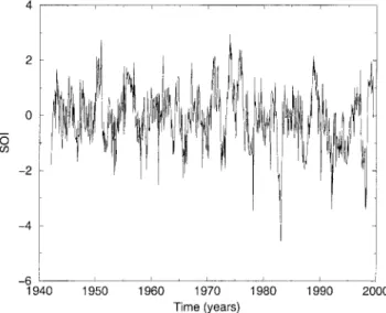
we shall turn to one of the best known climatic time series. This time series is made up of monthly values of the Southern Oscillation Index (SOI). It will be intro-duced in section 2.2 and is shown in Figure 2 there.

[4] At this point we merely note that physical

pro-cesses usually operate in continuous time. Most mea-surements, though, are done and recorded in discrete time. Thus the SOI time series, as well as most climatic and other geophysical time series, are available in dis-crete time.

1.1. Analysis in the Time Domain Versus the Spectral Domain

[5] Two basic approaches to time series analysis are

associated with the time domain or the spectral domain. We present them at first in the linear context in which the physical sciences have operated for most of the last two centuries. In this context the physical system can be described by a linear ordinary differential equation

(ODE), or a system of such equations, subject to addi-tive random forcing.

[6] It goes well beyond the scope of this review paper

to introduce the concepts of random variables, stochastic processes, and stochastic differential equations. We re-fer the interested reader to Feller [1968, 1971] for the former two concepts and to Arnold [1974] and Schuss [1980] for the latter. Many of the standard books on classical spectral methods that are cited in sections 3.1 and 3.2 also contain good elementary introductions to stochastic processes in discrete and, sometimes, contin-uous time.

[7] We concentrate here on time series in discrete

time and consider therefore first the simple case of a scalar, linear ordinary difference equation with random forcing,

X共t ⫹ 1兲 ⫽

冘

M

ajX共t ⫺ M ⫹ j兲 ⫹ ␴␰共t兲. (1) Its constant coefficients ajdetermine the solutions X(t) at discrete times t_{⫽ 0, 1, 䡠 䡠 䡠 , n, 䡠 䡠 䡠 . In (1) the random} forcing ␰(t) is assumed to be white in time, i.e.,

uncor-TABLE 1. (continued)

Symbol Definition Method Section

n⌬t discretely sampled time 1

Uk(f) discrete Fourier transform of wk(t) MTM 3.4

W sliding-window length of wavelet SSA 2.4 W␺(a, b) wavelet transform of {X(t)} using b-translated and a-dilated␺((t ⫺ b)/a) SSA 2.4

W␮(k) lag window for SញX(f) with smoothing parameter␮ BT 3.2

Wm(k) Bartlett window for SញX(f) with window length m BT 3.2

wk(t) kth taper MTM 3.4

Xˆ(t) observed time series 1

Xn X(n⌬t) 1

X(p) _{pth-order differentiation of X(t) with respect to time t, d}p_X/dtp ₁

{X(t)} univariate time series in t 僆 ⺢ or t 僆 ⺪⫹ ₁

X

˜(t) M-dimensional augmented vector of X(t) 2.1

X0 mean of {X(t)} SSA 2.3

XI(t) reconstructed X(t) WLTs 2.4

X

˜(t), X˜(n⌬t) continuous- and discrete-time reconstructed signal MTM 3.4 {X(t)} multivariate time series in t僆 ⺢ or t 僆 ⺪⫹ _{POP 4.1}

{X˜l} multichannel augmented vector of {X˜(t)} SSA 4.2

Yˆk(f) discrete Fourier transform of {X(t)wk(t)} MTM 3.4

␣ time-scale ratio SSA 2.4

␩(t) additive noise MTM 3.4

␪ explained contribution to variance MTM 3.4 ␭k, ⌳X kth eigenvalue and eigenvalue matrix of CX SSA 2.2

⌳R projection of CRonto EX SSA 2.3

␮k weight of kth taper MTM 3.4

␯ number of degrees of freedom of spectrum MTM 3.4

␰(t) random forcing 1

␳k, EX kth eigenvector and eigenvector matrix of CX SSA 2.2

␴2 _{variance of random forcing 1}

␶ characteristic delay time SSA 2.3

␾X(k),␾ˆX(k) true and estimated lag k autocorrelation function of X(t) BT 3.2

␺(x) mother wavelet of variable x WLTs 2.4 ␺ unexplained contribution to variance MTM 3.4

related from t to t ⫹ 1, and Gaussian at each t, with constant variance equal to unity. In the Yule [1927] and Walker [1931] method for the time domain approach, one computes the coefficients aj and the variance ␴2 from a realization of X having length N, {X(t)⬊1 ⱕ t ⱕ N }.

[8] This method is discussed further in section 3.3

below, where (1) is treated as an autoregressive (AR) process of order M, which we denote by AR(M). The notation used in the present paper is summarized in Table 1. The table lists the main symbols in alphabetical order and indicates the section where each symbol is introduced first. This facilitates the comparison between the methods we review, since the literature of each method tends to use its own notation.

[9] The spectral domain approach is motivated by the

observation that the most regular, and hence predict-able, behavior of a time series is to be periodic. This approach then proceeds to determine the periodic com-ponents embedded in the time series by computing the associated periods, amplitudes, and phases, in this order. [10] The classical implementation of the spectral

do-main approach is based on the Bochner-Khinchin-Wie-ner theorem [Box and Jenkins, 1970], which states that the lag autocorrelation function of a time series and its spectral density are Fourier transforms of each other. Hannan’s [1960] introduction to this approach and its implementation excels by its brevity and clarity; the so-called Blackman-Tukey implementation is presented in section 3.2 below. We shall use here both the more mathematical term of spectral density and the term of power spectrum, often encountered in the scientific and engineering literature, according to whether the context is more theoretical or more applied.

[11] The remainder of this review is organized as

follows. Section 2 deals mainly with signal-to-noise (S/N) ratio enhancement and introduces singular spectrum analysis (SSA) as an important and flexible tool for this enhancement. Connections between SSA and empirical orthogonal functions (EOFs) are outlined in Appendix A. Statistical tests for the reliability of SSA results are also discussed in this section, along with connections to wavelet analysis.

[12] In section 3 we present, in succession, three

methods of spectral analysis: Fourier transform based, maximum entropy, and multitaper. Both sections 2 and 3 use the SOI time series for the purposes of illustrating the methods “in action.” In section 4 the multivariate extensions of the maximum entropy method and of single-channel SSA are introduced, and a few additional applications are mentioned or illustrated. The review concludes with a section on open questions, from the point of view of both the methodology and its applica-tions.

1.2. Time Series and Nonlinear Dynamics

[13] Before proceeding with the technical details, we

give in this section a quick perspective on the “nonlinear

revolution” in time series analysis. Irregularity in ob-served time series had traditionally been attributed to the above mentioned random “pumping” of a linear system by infinitely many (independent) degrees of free-dom (DOF). In the 1960s and 1970s the scientific com-munity found out that much of this irregularity could be generated by the nonlinear interaction of a few DOF [Lorenz, 1963; Smale, 1967; Ruelle and Takens, 1971]. This realization of the possibility of deterministic aperi-odicity or “chaos” [Gleick, 1987] created quite a stir.

[14] The purpose of this review is to describe briefly

some of the implications of this change in outlook for time series analysis, with a special emphasis on climatic time series. Many general aspects of nonlinear time series analysis are reviewed by Drazin and King [1992], Ott et al. [1994], and Abarbanel [1996]. We concentrate here on those aspects that deal with regularities and have proven most useful in studying climatic variability. [15] A connection between deterministically chaotic

time series and the nonlinear dynamics generating them was attempted fairly early in the young history of “chaos theory.” The basic idea was to consider specifically a scalar, or univariate, time series with apparently irregu-lar behavior, generated by a deterministic or stochastic system. This time series could be exploited, so the think-ing went, in order to ascertain, first, whether the under-lying system has a finite number of DOF. An upper bound on this number would imply that the system is deterministic, rather than stochastic, in nature. Next, we might be able to verify that the observed irregularity arises from the fractal nature of the deterministic sys-tem’s invariant set, which would yield a fractional, rather than integer, value of this set’s dimension. Finally, one could maybe reconstruct the invariant set or even the equations governing the dynamics from the data.

[16] This ambitious program [Packard et al., 1980;

Roux et al., 1980; Ruelle, 1981] relied essentially on the method of delays, based in turn on the Whitney [1936] embedding lemma and the Man˜e´ [1981] and Takens [1981] theorems. We first describe an easy connection between a univariate and a multivariate time series.

[17] Let us assume that the univariate time series is

the solution of a scalar nonlinear ODE of order p, X共 p兲_{⫽ G共X}共 p⫺1兲_{, . . . , X兲. (2)}

This scalar higher-dimensional equation is equivalent to the following system of first-order ODEs:

X˙i⫽ Fi共X1, . . . , Xj, . . . , Xp兲, 1 ⱕ i, j ⱕ p; (3)

here X˙⬅ dX/dt ⬅ X(1)_{and X}( p)_{⬅ d}p_X/dtp_{. It suffices} to write

X⬅ X1, X˙1⫽ X2, . . . , X˙p⫺1⫽ Xp, X˙p⫽ G共X1, . . . , Xp兲,

(4) so that F1⫽ X2, F2⫽ X3, 䡠 䡠 䡠 , Fp⫽ G. In other words, the successive derivatives of X(t) can be thought of as the components of a vector X ⬅ (X1, 䡠 䡠 䡠 , Xp). The

Euclidean space⺢p_{in which the vector X⫽ X(t) evolves} is called the phase space of the first-order system (3). The graph of this evolution in ⺢p_{is called an orbit or a} trajectory of equation (3).

[18] Let us now change the point of view and consider

system (3) for arbitrary right-hand sides Fi(X), rather than for the specific Fi given by (4). Such an ODE system represents a fairly general description of a dif-ferentiable dynamical system in continuous time [Ar-nold, 1973, 1983]. We are interested at first in the case in which only a single time series Xˆ(t) is known, where Xˆ⫽ Xi for some fixed component i ⫽ i0 or Xˆ is some

sufficiently smooth function of all the components Xi. For the solutions of such a system to be irregular, i.e., other than (asymptotically) steady or periodic, three or more DOF are necessary. Can one then go from (3) to (2) just as easily as in the opposite direction? The answer, in general is no; hence a slightly more sophisti-cated procedure needs to be applied.

[19] This procedure is called the method of delays,

and it tries, in some sense, to imitate the Yule-Walker inference of (1) from the time series {X(t)_{⬊t ⫽ 1, 䡠 䡠 䡠 ,} N }. First of all, one acknowledges that the data X(t) are typically given at discrete times t ⫽ n⌬t only. Next, one admits that it is hard to actually get the right-hand sides Fi; instead, one attempts to reconstruct the invariant set on which the solutions of (3) that satisfy certain con-straints lie.

[20] In the case of conservative, Hamiltonian systems

[Lichtenberg and Lieberman, 1992], there are typically unique solutions through every point in phase space. The irregularity in the solutions’ behavior is associated with the intricate structure of cantori [Wiggins, 1988], complicated sets of folded tori characterized by a given energy of the solutions lying on them. These cantori have, in particular, finite and fractional dimension, being self-similar fractals [Mandelbrot, 1982].

[21] Mathematically speaking, however, Hamiltonian

systems are structurally unstable [Smale, 1967] in the function space of all differentiable dynamical systems. Physically speaking, on the other hand, “open” systems, in which energy is gained externally and dissipated in-ternally, abound in nature. Therefore climatic time se-ries, as well as most other time series from nature or the laboratory, are more likely to be generated by forced dissipative systems [Lorenz, 1963; Ghil and Childress, 1987, chapter 5]. The invariant sets associated with ir-regularity here are “strange attractors” [Ruelle and Tak-ens, 1971], toward which all solutions tend asymptoti-cally; that is, long-term irregular behavior in such systems is associated with these attractors. These objects are also fractal, although rigorous proofs to this effect have been much harder to give than in the case of Hamiltonian cantori [Guckenheimer and Holmes, 1983; Lasota and Mackey, 1994].

[22] Man˜e´ [1981], Ruelle [1981], and Takens [1981]

had the idea, developed further by Sauer et al. [1991], that a single observed time series Xˆ(t) (where Xˆ ⫽ Xi0

or, more generally, Xˆ ⫽ ␾(X1(t), 䡠 䡠 䡠 , Xp(t))) could be used to reconstruct the attractor of a forced dissipative system. The basis for this reconstruction idea is essen-tially the fact that the solution that generates X(t) covers the attractor densely; that is, as time increases, this solution will pass arbitrarily close to any point on the attractor. Time series observed in the natural environ-ment, however, have finite length and sampling rate, as well as significant measurement noise.

[23] The embedding idea has been applied therefore

most successfully to time series generated numerically or by laboratory experiments in which sufficiently long se-ries could be obtained and noise was controlled better than in nature. Broomhead and King [1986a], for in-stance, successfully applied SSA to the reconstruction of the Lorenz [1963] attractor. As we shall see, for climate and other geophysical time series, it might be possible to attain a more modest goal: to describe merely a “skele-ton” of the attractor that is formed by a few robust periodic orbits.

[24] In the climate context, Lorenz [1969] had already

pointed out a major stumbling block for applying the attractor reconstruction idea to large-scale atmospheric motions. While using more classical statistical methods, he showed that the recurrence time of sufficiently good analogs for weather maps was of the order of hundreds of years, at the spatial resolution of the observational network then available for the Northern Hemisphere.

[25] The next best target for demonstrating from an

observed time series the deterministic cause of its irreg-ularity was to show that the presumed system’s attractor had a finite and fractional dimension. Various dimen-sions, metric and topological, can be defined [Kaplan and Yorke, 1979; Farmer et al., 1983]; among them, the one that became the most popular, since easiest to compute, was the correlation dimension [Grassberger and Procaccia, 1983]. In several applications, its compu-tation proved rather reliable and hence useful. Climatic time series, however, tended again to be rather too short and noisy for comfort (see, for instance, Ruelle [1990] and Ghil et al. [1991] for a review of this controversial topic).

[26] A more robust connection between classical

spec-tral analysis and nonlinear dynamics seems to be pro-vided by the concept of “ghost limit cycles.” The road to chaos [Eckmann, 1981] proceeds from stable equilibria, or fixed points, through stable periodic solutions, or limit cycles, and on through quasiperiodic solutions lying on tori, to strange attractors. The fixed points and limit cycles are road posts on this highway from the simple to the complex. That is, even after having lost their stability to successively more complex and realistic solutions, these simple attractors still play a role in the observed spatial patterns and the time series generated by the system.

[27] A “ghost fixed point” is a fixed point that has

become unstable in one or a few directions in phase space. Still, the system’s trajectories will linger near it for

extended time intervals [Legras and Ghil, 1985]. Like-wise, a ghost limit cycle is a closed orbit that has become slightly unstable but is visited, again and again, by the system’s trajectories [Kimoto and Ghil, 1993].

[28] Consider the periodic solution shown in Figure

1a as embedded in Euclidean three-dimensional phase space. It is neutrally stable in the direction tangent to itself, while in the plane perpendicular to this tangent it is asymptotically stable in one direction and unstable in the other, as shown in the Poincare´ section of Figure 1b. In a multidimensional phase space it is plausible that the directions of stability are numerous or even infinite in number. The directions of instability, however, would still be few in number, for parameter values not too far from those at which the Hopf bifurcation that gave rise to the limit cycle in the first place occurs. Hence solu-tions of the full system would easily be attracted to this barely unstable limit cycle, follow it closely for one or a few turns, be ejected from its neighborhood, only to return later, again and again.

[29] The analogous picture for a ghost fixed point was

illustrated in detail for an atmospheric model with 25 DOF by Legras and Ghil [1985; see also Ghil and Chil-dress, 1987, Figures 6.12 and 6.18]. Thus the “ghosts” of fixed points and limit cycles leave their imprint on the system’s observed spatiotemporal behavior.

[30] The episodes during which the system trajectory

circles near a ghost limit cycle result in nearly periodic segments of the time series and hence contribute to a spectral peak with that period. This concept was illus-trated using 40 years of an atmospheric multivariate time series by Kimoto and Ghil [1993] for the so-called in-traseasonal oscillations of the Northern Hemisphere [see also Ghil and Mo, 1991a]. We shall show in the subsequent sections of the present review, in particular

section 2.2, how this concept can be generalized to associate multiple spectral peaks with a robust skeleton of the attractor, as proposed by Vautard and Ghil [1989].

2. ENHANCING THE SIGNAL-TO-NOISE (S/N) RATIO

2.1. Motivation for Singular Spectrum Analysis (SSA)

[31] SSA is designed to extract information from short

and noisy time series and thus provide insight into the unknown or only partially known dynamics of the un-derlying system that generated the series [Broomhead and King, 1986a; Fraedrich, 1986; Vautard and Ghil, 1989]. We outline here the method for univariate time series and generalize for multivariate ones in section 4.2. [32] The analogies between SSA and spatial EOFs are

summarized in Appendix A, along with the basis of both in the Karhunen-Loe`ve theory of random fields and of stationary random processes. Multichannel SSA (see section 4.2) is numerically analogous to the extended EOF (EEOF) algorithm of Weare and Nasstrom [1982]. The two different names arise from the origin of the former in the dynamical systems analysis of univariate time series, while the latter had its origins in the princi-pal component analysis of meteorological fields. The two approaches lead to different methods for the choice of key parameters, such as the fixed or variable window width, and hence to differences in the way of interpret-ing results.

[33] The starting point of SSA is to embed a time

series {X(t)_{⬊t ⫽ 1, 䡠 䡠 䡠 , N} in a vector space of} dimen-sion M, i.e., to represent it as a trajectory in the phase space of the hypothetical system that generated {X(t)}. In concrete terms this is equivalent to representing the behavior of the system by a succession of overlapping “views” of the series through a sliding M-point window. [34] Let us assume, for the moment, that X(t) is an

observable function Xˆ(t) of a noise-free system’s depen-dent variables Xi(t), as defined in (4), and that the function ␾ that maps the p variables {Xi(t)_{⬊i ⫽ 1, 䡠 䡠 䡠 ,} p} into the single variable X(t) has certain properties that make it generic in the dynamical systems sense of Smale [1967]. Assume, moreover, that M ⬎ 2d ⫹ 1, where d is the dimension of the underlying attractor on which the system evolves, and that d is known and finite. If so, then the representation of the system in the “delay coordinates” described in (5) below will share key topo-logical properties with a representation in any coordi-nate system. This is a consequence of Whitney’s [1936] embedding lemma and indicates the potential value of SSA in the qualitative analysis of the dynamics of non-linear systems [Broomhead and King, 1986a, 1986b; Sauer et al., 1991]. The quantitative interpretation of SSA results in terms of attractor dimensions is fraught with difficulties, however, as pointed out by a number of authors [Broomhead et al., 1987; Vautard and Ghil, 1989; Palus˘ and Dvor˘a´k, 1992].

Figure 1. Schematic diagram of a ghost limit cycle. Figure 1a is a perspective sketch of the limit cycle (bold curve) in a three-dimensional Euclidean space. Light solid curves indicate two distinct trajectories that approach the limit cycle in a direction in which it is stable and leave its neighborhood in an unstable direction. Figure 1b is a sketch of the projection of four representative trajectories (light curves) onto a Poincare´ section (i.e., a plane intersecting transversally the limit cycle) in a neighborhood of the limit cycle. The figure’s mutually per-pendicular directions (bold lines) of stability (inward pointing arrows) and instability (outward pointing arrows) can form, in general, an arbitrary angle with each other. The shape of such a limit cycle need not be elliptic, as shown in the figure, except near the Hopf bifurcation point where it arises. Reprinted from Ghil and Yiou [1996] with permission of Springer-Verlag.

[35] We therefore use SSA here mainly (1) for

data-adaptive signal-to-noise (S/N) enhancement and associ-ated data compression and (2) to find the attractor’s skeleton, given by its least unstable limit cycles (see again Figure 1 above). The embedding procedure ap-plied to do so constructs a sequence {X˜(t)} of M-dimensional vectors from the original time series X, by using lagged copies of the scalar data {X(t)⬊1 ⱕ t ⱕ N },

X

˜共t兲 ⫽ 共X共t兲, X共t ⫹ 1兲, . . . , X共t ⫹ M ⫺ 1兲兲; (5) the vectors X˜(t) are indexed by t ⫽ 1, 䡠 䡠 䡠 , N⬘, where N⬘ ⫽ N ⫺ M ⫹ 1.

[36] SSA allows one to unravel the information

em-bedded in the delay-coordinate phase space by decom-posing the sequence of augmented vectors thus obtained into elementary patterns of behavior. It does so by providing data-adaptive filters that help separate the time series into components that are statistically inde-pendent, at zero lag, in the augmented vector space of interest. These components can be classified essentially into trends, oscillatory patterns, and noise. As we shall see, it is an important feature of SSA that the trends need not be linear and that the oscillations can be amplitude and phase modulated.

[37] SSA has been applied extensively to the study of

climate variability, as well as to other areas in the phys-ical and life sciences. The climatic applications include the analysis of paleoclimatic time series [Vautard and Ghil, 1989; Yiou et al., 1994, 1995], interdecadal climate variability [Ghil and Vautard, 1991; Allen and Smith, 1994; Plaut et al., 1995; Robertson and Mechoso, 1998], as well as interannual [Rasmusson et al., 1990; Keppenne and Ghil, 1992] and intraseasonal [Ghil and Mo, 1991a, 1991b] oscillations. SSA algorithms and their properties have been investigated further by Penland et al. [1991], Allen [1992], Vautard et al. [1992], and Yiou et al. [2000]. The SSA Toolkit first documented by Dettinger et al. [1995a] was built, largely but not exclusively, around this technique.

2.2. Decomposition and Reconstruction

[38] In this section we illustrate the fundamental SSA

formulae with the classical example of a climatic time series, the Southern Oscillation Index (SOI). SOI is a climatic index connected with the recurring El Nin˜o conditions in the tropical Pacific. It is defined usually as the difference between the monthly means of the sea level pressures at Tahiti and at Darwin (Australia). We use this definition and the monthly data given in the archive http://tao.atmos.washington.edu/pacs/additional_ analyses/soi.html.

[39] The SOI data in this archive are based on the

time series at each of the two stations being deseason-alized and normdeseason-alized [Ropelewski and Jones, 1987]. The seasonal cycle is removed by subtracting the average of the values for each calendar month over a reference

interval, in this case 1951–1980. The residues from this operation, called monthly anomalies in the climatologi-cal literature, are then normalized with respect to the standard deviation computed over the same interval.

[40] The archived SOI data for 1866–1997 are from

the Climate Research Unit of the University of East Anglia, and those for 1998–1999 are from the Climate Prediction Center of the U.S. National Centers for En-vironmental Prediction (NCEP). They are obtained by taking the difference between the anomalies at Tahiti and those at Darwin and dividing by the standard devi-ation of this difference over the same 30-year reference interval. The time interval we consider here goes from January 1942 to June 1999, during which no observations are missing at either station; this yields N ⫽ 690 raw data points. Note that this raw SOI time series is cen-tered and normalized over the reference interval 1951– 1980, but not over the entire interval of interest. We show in Figure 2 the SOI obtained from this raw data set. It actually has mean⫺0.0761 and standard deviation equal to 1.0677. All subsequent figures, however, use a version of the series that has been correctly centered over the interval January 1942 to June 1999.

[41] SSA is based on calculating the principal

direc-tions of extension of the sequence of augmented vectors {X˜(t)⬊t ⫽ 1, 䡠 䡠 䡠 , N⬘} in phase space. The M ⫻ M covariance matrix CXcan be estimated directly from the data as a Toeplitz matrix with constant diagonals; that is, its entries cij depend only on the lag兩i ⫺ j兩 [cf. Vautard and Ghil, 1989]:

cij⫽_{N⫺ 兩i ⫺ j兩}1

冘

N⫺兩i⫺j兩

X共t兲 X共t ⫹ 兩i ⫺ j兩兲. (6) The eigenelements {(␭k,␳k)_{⬊k ⫽ 1, 䡠 䡠 䡠 , M} of C}Xare then obtained by solving

Figure 2. Variations of the Southern Oscillation Index (SOI) between January 1942 and June 1999. Time on the abscissa is in calendar years, and SOI on the ordinate is normalized by its standard deviation.

CX␳k⫽ ␭k␳k. (7) The eigenvalue ␭k equals the partial variance in the direction␳k, and the sum of the␭k, i.e., the trace of C_X, gives the total variance of the original time series X(t). [42] An equivalent formulation of (7), which will

prove useful further on, is given by forming the M ⫻ M matrix E_Xthat has the eigenvectors␳kas its columns and the diagonal matrix ⌳X whose elements are the eigen-values␭k, in decreasing order:

EXtCXEX⫽ ⌳X; (8)

here EXt is the transpose of EX. Each eigenvalue␭kgives the degree of extension, and hence the variance, of the time series in the direction of the orthogonal eigenvector ␳k.

[43] A slightly different approach to computing the

eigenelements of CXwas originally proposed by Broom-head and King [1986a]. They constructed the N⬘ ⫻ M trajectory matrix D that has the N⬘ augmented vectors

X

˜(t) as its rows and used singular-value decomposition (SVD) [see, for instance, Golub and Van Loan, 1996] of

CX⫽ 1

N⬘DtD (9)

to obtain the square roots of␭k. The latter are called the singular values of D and have given SSA its name.

[44] Allen and Smith [1996] and Ghil and Taricco

[1997] have discussed the similarities and differences between the approaches of Broomhead and King [1986a] and Vautard and Ghil [1989] in computing the eigenele-ments associated in SSA with a given time series X(t). Both the Toeplitz estimate (6) and the SVD estimate (9) lead to a symmetric covariance matrix CX. In addition, the eigenvectors ␳k of a Toeplitz matrix are necessarily odd and even, like the sines and cosines of classical Fourier analysis. The Toeplitz approach has the advan-tage of better noise reduction when applied to short time series, as compared with the SVD approach. This ad-vantage comes at the price of a slightly larger bias when the time series is strongly nonstationary over the interval of observation 1 ⱕ t ⱕ N [Allen, 1992]. Such bias-versus-variance trade-offs are common in estimation problems.

[45] To obtain S/N separation, one plots the

eigen-value spectrum illustrated in Figure 3. In this plot an initial plateau that contains most of the signal is sepa-rated by a steep slope from the noise; the latter is characterized by much lower values that form a flat floor or a mild slope [Kumaresan and Tufts, 1980; Pike et al., 1984; Vautard and Ghil, 1989].

[46] As the M⫻ M matrix CXis symmetric, standard

algorithms [Press et al., 1988] will perform its spectral decomposition efficiently, as long as M is not too large. The choice of M is based on a trade-off between two considerations: quantity of information extracted versus the degree of statistical confidence in that information.

The former requires as wide a window as possible, i.e., a large M, while the latter requires as many repetitions of the features of interest as possible, i.e., as large a ratio N/M as possible. The choice of M ⫽ 60 in Figure 3 allows us to capture periodicities as long as 5 years, since ⌬t ⫽ 1 month, and thus the dimensional window width is M⌬t ⫽ 5 years; on the other hand, N/M ⬵ 11 is fairly safe, and the diagonalization of CX for this moderate value of M does not introduce large numerical errors either.

[47] In Figure 3, there is a clear grouping of the first

five eigenvalues, followed by a very steep slope of three additional eigenvalues. The latter are well separated from the first five, as well as from the remaining 52 eigenvalues, which form the mildly sloping and flattening out “tail” of the SSA spectrum.

[48] The S/N separation obtained by merely

inspect-ing the slope break in a “scree diagram” of eigenvalues ␭kor singular values␭k1/ 2versus k works well when the intrinsic noise that perturbs the underlying deterministic system and the extrinsic noise that affects the observa-tions are both white, i.e., uncorrelated from one time step to the next (see definition of␰(t) in equation (1)). This rudimentary separation works less well when either

Figure 3. Singular spectrum of the SOI time series. The eigenvalues are plotted, as usual, in decreasing order. The embedding dimension for Figures 3–7 is M ⫽ 60, which represents a time window of 5 years. The error bars are based on the default option of the singular spectrum analysis (SSA) multitaper method (MTM) Toolkit (http://www.atmos.u-cla.edu/tcd/ssa/). This option uses the ad hoc estimate of vari-ance␴k of an eigenvalue␭kgiven by␴k⫽ (2/Nˆ)␭k. The key

element of this estimate is the number Nˆ of independent degrees of freedom (DOF) in the time series. Vautard and Ghil [1989], who first proposed this estimate in SSA, used Nˆ ⫽ N, which is very optimistic, while Ghil and Mo [1991a] used Nˆ ⫽ N/M, which is too conservative. The Toolkit’s current Version 4.0, following Unal and Ghil [1995], uses Nˆ ⫽ N/␬␶, where ␶ is the time series’ estimated decorrelation time (see equations (15) and (16)) and␬ is an empirical constant, ␬ ⫽ 1.5.

noise is red, i.e., when it is given by an AR(1) process (see section 3.3) or is otherwise correlated between time steps [Vautard and Ghil, 1989]. The difficulties that arise with correlated noise led Allen [1992] and Allen and Smith [1994] to develop Monte Carlo SSA (see section 2.3).

[49] When the noise properties can be estimated

re-liably from the available data, the application of a so-called “prewhitening operator” can significantly enhance the signal separation capabilities of SSA [Allen and Smith, 1997]. The idea is to preprocess the time series itself or, equivalently but often more efficiently, the lag covariance matrix CX, such that the noise becomes un-correlated in this new representation. SSA is then per-formed on the transper-formed data or covariance matrix and the results are transformed back to the original representation for inspection.

[50] By analogy with the meteorological literature, the

eigenvectors ␳k of the lag covariance matrix CX have been called empirical orthogonal functions (EOFs) [see Preisendorfer, 1988, and references therein] by Fraedrich [1986] and by Vautard and Ghil [1989]. The EOFs cor-responding to the first five eigenvalues are shown in Figure 4. Note that the two EOFs in each one of the two leading pairs, i.e., EOFs 1 and 2 (Figure 4a) as well as EOFs 3 and 4 (Figure 4b), are in quadrature and that each pair of EOFs corresponds in Figure 3 to a pair of eigenvalues that are approximately equal and whose error bars overlap. Vautard and Ghil [1989] argued that subject to certain statistical significance tests discussed further below, such pairs correspond to the nonlinear counterpart of a sine-cosine pair in the standard Fourier analysis of linear problems.

[51] In the terminology of section 1 here, such a pair

gives a handy representation of a ghost limit cycle. The advantage over sines and cosines is that the EOFs

obtained from SSA are not necessarily harmonic func-tions and, being data adaptive, can capture highly anharmonic oscillation shapes. Indeed, relaxation os-cillations [Van der Pol, 1940] and other types of non-linear oscillations [Stoker, 1950], albeit purely peri-odic, are usually not sinusoidal; that is, they are anharmonic. Such nonlinear oscillations often require therefore the use of many harmonics or subharmonics of the fundamental period when carrying out classical Fourier analysis, while a single pair of SSA eigen-modes might suffice. Capturing the shape of an an-harmonic oscillation, such as a seesaw or boxcar, albeit slightly rounded or smoothed, is easiest when the SSA window is exactly equal to the single period being analyzed.

[52] Projecting the time series onto each EOF yields

the corresponding principal components (PCs) A_k: Ak共t兲 ⫽

冘

j⫽1

M

X共t ⫹ j ⫺ 1兲␳k共 j兲. (10) Figure 5 shows the variations of the five leading PCs. Again, the two PCs in each of the pairs (1, 2) and (3, 4) are in quadrature, two by two (see Figures 5a and 5b). They strongly suggest periodic variability at two different periods, of about 4 and 2 years, respectively. Substantial amplitude modulation at both periodicities is present, too.

[53] The fifth PC, shown in Figure 5c, contains both a

long-term, highly nonlinear trend and an oscillatory component. We shall discuss the trend of the SOI series in connection with Figures 6b and 16a further below.

[54] We can reconstruct that part of a time series that Figure 4. First five empirical orthogonal functions (EOFs) of

the SOI time series. The leading four EOFs are grouped into two pairs, (1, 2) and (3, 4), in Figures 4a and 4b.

Figure 5. First five principal components (PCs) of the SOI time series. Note phase quadrature in Figures 5a and 5b. The maximal cross correlation in Figure 5a is reached when PC-2 leads PC-1 by 10 months and equals 0.89. In Figure 5b the maximum cross correlation equals 0.71 and is obtained when PC-4 leads PC-3 by 9 months.

is associated with a single EOF or several by combining the associated PCs: R᏷共t兲 ⫽ 1 Mt_k

冘

冘

冦

冉

冊

冉

冊

冉

冊

[55] The reconstructed components (RCs) have the

property of capturing the phase of the time series in a well-defined least squares sense, so that X(t) and R_᏷(t) can be superimposed on the same timescale, 1ⱕ t ⱕ N. This is an advantage of the RCs over the PCs, which have length N ⫺ M and do not contain direct phase information within the window width M.

[56] No information is lost in the reconstruction

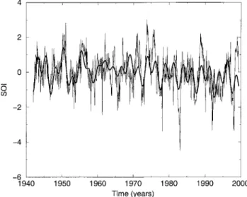
pro-cess, since the sum of all individual RCs gives back the original time series. Partial reconstruction is illustrated in Figure 6 by summing the variability of PCs 1–4, associated with the two leading pairs of eigenelements; it is common to refer to such a reconstruction (equation (11)), with᏷ ⫽ {1, 2, 3, 4}, as RCs 1–4. The portion of the SOI variability thus reconstructed contains 43% of the total variance. It captures the quasi-oscillatory be-havior isolated by these two leading pairs, with its two distinct near-periodicities.

[57] It is clear that the partial SOI reconstruction

(bold curve in Figure 6a) is smooth and represents the essential part of the interannual variability in the monthly SOI data (thin curve). Each of the two pairs of RCs, 1–2 and 3–4, can be thought of as retracing a ghost limit cycle in the phase space of the tropical climate system. These two limit cycles can then be said to form the robust skeleton of the attractor. It is unlikely that a time series of a few hundred points, like the SOI or other typical climatic time series, will suffice to capture the attractor’s fine structure [Vautard and Ghil, 1989].

[58] This robust skeleton, however, provides sufficient

information for most practical purposes. In particular, warm events (El Nin˜os) and cold ones (La Nin˜as) over the eastern tropical Pacific are captured quite well, dur-ing the 57.5 years of record, as minima and maxima of the partially reconstructed SOI. We check this statement by comparing the bold curve in Figure 6a with the vertical arrows along the figure’s upper and lower ab-scissae.

[59] These arrows correspond to strong (bold arrows)

or moderate (light arrows) El Nin˜o–Southern Oscillation (ENSO) events. The events are defined subjectively, calendar quarter by calendar quarter, from reanalyzed surface temperature data produced at NCEP and the U.K. Met. Office for the years 1950–1999 (see http:// www.cpc.noaa.gov/products/analysis_monitoring/ensostuff/ ensoyears.html).

[60] Large positive peaks in the partial SOI

recon-struction, i.e., those that exceed one standard deviation, match the strong La Nin˜as quite well (downward point-ing arrows on the upper abscissa). The only exceptions are the 1950 and 1971 cold events, which were of mod-erate strength, and the weak 1996 La Nin˜a.

[61] The same good match obtains between the large

negative peaks in the figure’s bold curve, i.e., those that exceed one standard deviation, and the strong El Nin˜os (upward pointing arrows on the lower abscissa). The only notable exception is the large peak in 1977–1978, which was classified subjectively as a weak warm event.

Figure 6. Partial reconstructions of the SOI time series. Fig-ure 6a is a reconstruction based on EOFs 1–4 (bold curve). The raw SOI series is shown as the light curve. El Nin˜os (warm events) are shown as upward pointing arrows on the lower abscissa, while La Nin˜as (cold events) are shown as downward pointing arrows on the upper abscissa; the arrows are aligned with the January closest to the event maximum. Figure 6b shows the trend of reconstructed component (RC) number 5 (RC-5); see text for details.

The 1957–1958 and 1991–1992 events appear as moder-ate-size minima in the partial SOI reconstruction. They are included in the NCEP list as strong El Nin˜os for one (January–March 1958) or two (January–June 1992) sea-sons, but neither was strong during the second half of the calendar year. Thus the only discrepancies among the oscillatory part of the SOI, based on RCs 1– 4, and the subjective NCEP classification are in the intensi-ties (moderate versus strong, or vice versa) of a few events.

[62] Earlier SSA results do support the present

em-phasis on the doubly periodic character of ENSO phe-nomena. They include the analyses of Rasmusson et al. [1990] for sea surface temperatures and near-surface zonal winds in the tropical Indo-Pacific belt, those of Keppenne and Ghil [1992] for a slightly different treat-ment of the SOI, as well as those of Jiang et al. [1995a] for sea surface temperatures and of Unal and Ghil [1995] for sea level heights in the tropical Pacific. In all these data sets and SSA analyses, a quasi-biennial and a lower-frequency, quasi-quadrennial oscillatory pair were reli-ably identified among the leading SSA eigenelements.

[63] Shown in Figure 6b is also a filtered version of

RC-5, which captures well the small but significant long-term trend of the SOI time series in Figure 2. To eliminate the oscillatory component apparent in PC-5 (Figure 5c), we applied SSA with the same 60-month window to the full RC-5. The two leading eigenmodes correspond to a pure trend, shown in Figure 6b, while the second eigenpair corresponds to a quasi-biennial oscillation (not shown). The SOI trend in Figure 6b agrees, up to a point, with the one captured by the multitaper reconstruction in section 3.4.2 (see Figure 16a there). Given the recent interest in the interdecadal variability of ENSO, we postpone further discussion of this result for the moment when its multitaper version is also in hand.

[64] Reliable S/N separation and identification of

os-cillatory pairs is not always as easy as in the case of interannual climate variability in the tropical Pacific. Global surface-air temperatures, for instance, present a considerably more difficult challenge for identifying in-terannual and interdecadal oscillations. Elsner and Tso-nis’s [1991] excessive reliance on eigenvalue rank order as a criterion of significance in SSA has led to consider-able confusion in this case [see Allen et al., 1992a, 1992b]. [65] Reliable identification of the true signal conveyed

by a short, noisy time series and of the oscillatory com-ponents within this signal requires effective criteria for statistical significance, which are treated in the next section. Subject to these caveats, a clean signal, obtained by partial reconstruction over the correct set of indices ᏷, provides very useful information on the underlying system, which is often poorly or incompletely known.

[66] Such a signal can then be analyzed further, both

visually and by using other spectral analysis tools that are described in section 3. The maximum entropy method (MEM), which we describe in section 3.3, works

partic-ularly well on signals so enhanced by SSA [Penland et al., 1991].

2.3. Monte Carlo SSA

[67] In the process of developing a methodology for

applying SSA to climatic time series, a number of heu-ristic [Vautard and Ghil, 1989; Ghil and Mo, 1991a; Unal and Ghil, 1995] or Monte Carlo [Ghil and Vautard, 1991; Vautard et al., 1992] methods have been devised for S/N separation or the reliable identification of oscillatory pairs of eigenelements. They are all essentially attempts to discriminate between the significant signal as a whole, or individual pairs, and white noise, which has a flat spectrum. A more stringent “null hypothesis” [Allen, 1992] is that of red noise, since most climatic and other geophysical time series tend to have larger power at lower frequencies [Hasselmann, 1976; Mitchell, 1976; Ghil and Childress, 1987].

[68] For definiteness, we shall use here the term red

noise exclusively in its narrow sense, of an AR(1) process given by (1) with M ⫽ 1 and 0 ⬍ a1⬍ 1, as required by

weak or wide-sense stationarity (see Appendix A for an exact definition). Other stochastic processes that have a continuous spectral density S( f ) which decreases mono-tonically with frequency f will be called “warm colored.” [69] The power spectrum S( f ) of the AR(1) process

is given by [e.g., Chatfield, 1984] S共 f 兲 ⫽ S0

1⫺ r2

1⫺ 2r cos 共2␲f/fN兲 ⫹ r2. (13)

Here 0 ⬍ S0 ⬍ ⬁ is the average value of the power

spectrum, related to the white-noise variance␴2_{in (1) by}

S0⫽

␴2

1⫺ r2, (14)

while r is the lag-one autocorrelation, r ⫽ a1, and the

Nyquist frequency fN⫽ 1/(2⌬t) is the highest frequency that can be resolved for the sampling rate⌬t. Note that in (1) and (5) we have used ⌬t ⫽ 1 for simplicity and without loss of generality, since ⌬t can always be rede-fined as the time unit. It is useful at this point to recall, for clarity’s sake, that it is not necessary to do so. The characteristic decay timescale␶ of the AR(1) noise can be estimated by

␶ ⫽ ⫺_{log r .}⌬t (15)

[70] In general, straightforward tests can be devised to

compare a given time series with an idealized noise process: The continuous spectrum of such a process is known to have a particular shape, and if a particular feature of the data spectrum lies well above this theo-retical noise spectrum, it is often considered to be sta-tistically “significant.” A single realization of a noise process can, however, have a spectrum that differs greatly from the theoretical one, even when the number of data points is large. It is only the (suitably weighted)

average of such sample spectra over many realizations that will tend to the theoretical spectrum of the ideal noise process. Indeed, the Fourier transform of a single realization of a red-noise process can yield arbitrarily high peaks at arbitrarily low frequencies; such peaks could be attributed, quite erroneously, to periodic com-ponents.

[71] More stringent tests have to be used therefore to

establish whether a time series can be distinguished from red noise or not. Allen [1992] devised such a test that compares the statistics of simulated red-noise time series with those of a given climatic time series. The principle of this test is implicit in some of Broomhead and King’s [1986a] ideas. The application of SSA in combination with this particular Monte Carlo test against red noise has become known as “Monte Carlo SSA” (MC-SSA) [see Allen and Smith, 1994, 1996].

[72] MC-SSA can be used, more generally, to

estab-lish whether a given time series can be distinguished from other well-defined processes. We only present here, for the sake of brevity and clarity, the original test against an AR(1) process. Allen [1992] proposes, in fact, to estimate the mean X0of the process at the same time

as the other parameters. We therefore rewrite (1) here for the particular case at hand as

X共t兲 ⫽ a1关X共t ⫺ 1兲 ⫺ X0兴 ⫹ ␴␰共t兲 ⫹ X0; (16)

here, as in (1),␰(t) is a Gaussian-distributed white-noise process with zero mean and unit variance.

[73] When testing against the process (16), the first

step in MC-SSA is to estimate the mean X0 and the

coefficients a1and␴ from the time series X(t) by using

a maximum likelihood criterion. Allen and Smith [1996] provide low-bias estimators that are asymptotically un-biased in the limit of large N and close to unun-biased for series whose length N is at least an order of magnitude longer than the decorrelation time ␶ ⫽ ⫺1/log r. Co-chrane and Orcutt [1949] have shown that when␶ is not very small relative to N, the use of a crude estimate for the mean X0, i.e., “centering” the time series first, can

lead to severe biases in the subsequent estimation of a1.

This is not the case for the SOI time series used here, as ␶ ⬍⬍ N for it. Hence we have used an SOI time series, based on the data in Figure 2, that has been centered.

[74] On the basis of estimated values Xˆ₀, aˆ₁, and␴ˆ of

these parameters, an ensemble of simulated red-noise data is generated and, for each realization, a covariance matrix CRis computed. In the nonlinear dynamics liter-ature, such simulated realizations of a noise process are often called surrogate data [Drazin and King, 1992; Ott et al., 1994].

[75] The covariance matrices of the surrogate data are

then projected onto the eigenvector basis EX of the original data by using (8) for their SVD,

⌳R⫽ EXt_C

REX. (17)

[76] Since (17) is not the SVD of the particular

real-ization CR, the matrix⌳Ris not necessarily diagonal, as

it is in (8). Instead, ⌳R measures the resemblance of a given surrogate set with the original data set of interest. The degree of resemblance can be quantified by com-puting the statistics of the diagonal elements of⌳R. The statistical distribution of these elements, determined from the ensemble of Monte Carlo simulations, gives confidence intervals outside which a time series can be considered to be significantly different from a random realization of the process (16). For instance, if an eig-envalue␭klies outside a 90% noise percentile, then the red-noise null hypothesis for the associated EOF (and PC) can be rejected with this level of confidence. Oth-erwise, that particular SSA component of the time series cannot be considered as significantly different from red noise. Additional problems posed by the multiplicity of SSA eigenvalues and other finer points are also dis-cussed by Allen [1992] and Allen and Smith [1996].

[77] As the next step in the analysis of our SOI time

series, we apply an MC-SSA noise test to it. In order to enhance the readability of the diagrams for the SSA spectra in the presence of MC-SSA error bars, we asso-ciate a dominant frequency with each EOF detected by SSA, as suggested by Vautard et al. [1992], and plot in Figure 7 the eigenvalues (diamonds) versus frequency, following Allen and Smith [1996].

[78] Such a plot is often easier to interpret, with

respect to the MC-SSA error bars, than plotting versus the eigenvalue’s rank k as in Figure 3. Care needs to be exercised, however, since the dominant-frequency esti-mate may be ambiguous or uncertain, due to the possi-ble anharmonicity of the EOFs, especially for low

fre-Figure 7. Monte Carlo singular spectrum of the SOI time series. The diamonds indicate projections of the noise eigen-vectors onto the data correlation matrix (see equation (17)); the lower and upper ticks on the error bars indicate the 5th and 95th noise percentiles. For each EOF, a characteristic fre-quency was estimated by maximizing its correlation with a sinusoid; therefore the frequency at which each diamond is plotted is just an average estimate. The frequencies in this figure and subsequent ones are given in cycles per month.

quencies. This is patently the case for the fifth mode in Figures 3–5. This mode appears at zero frequency in Figure 7, while we know very well that it has a quasi-biennial oscillatory component besides its capturing the SOI’s nonlinear trend.

[79] The error bars shown in Figure 7 for each EOF

represent 90% of the range of variance found in the state-space direction defined by that EOF in an ensem-ble of 1000 red-noise realizations; that is, it denotes the interval between the 5th and 95th percentile. Hence eigenvalues lying outside this interval are relatively un-likely (at the 10% level) to be due merely to the red-noise process (equation (16)) against which they are being tested.

[80] The high values in Figure 7 exhibit a significant

quasi-biennial oscillation and an oscillatory component with a period of about 50 months. The low values near 1 cycle yr⫺1_{are due to the fact that the seasonal cycle has}

been removed prior to the analysis, and the consequent suppression of power near annual-cycle periods has not been taken into account in the noise parameter estima-tion. Allen and Smith [1996] recommend that as far as possible, seasonal cycles should not be removed prior to the analysis, but that their presence should be taken into account explicitly in the parameter estimation [see also Jiang et al., 1995a; Unal and Ghil, 1995]. This recommen-dation has to be weighted against two related consider-ations. First, the reliable identification of a given peri-odicity becomes harder as the number of periodicities to be estimated increases, and second, the seasonal cycle and its physical causes are fairly well known and under-stood.

[81] The MC-SSA algorithm described above can be

adapted to eliminate known periodic components and test the residual against noise. This adaptation can pro-vide better insight into the dynamics captured by the data. Indeed, known periodicities, like orbital forcing on the Quaternary timescale or seasonal forcing on the intraseasonal-to-interannual one, often generate much of the variance at the lower frequencies manifest in a time series and alter the rest of the spectrum. Allen [1992] and Allen and Smith [1996] describe this refine-ment of MC-SSA which consists of restricting the pro-jections given by (17) to the EOFs that do not account for known periodic behavior.

[82] Monte Carlo simulation is a robust, flexible, and

nonparametric approach to assessing the significance of individual eigenmodes in SSA. Since it can be computa-tionally intensive, Allen and Smith [1996] suggest a much faster, albeit parametric alternative. In an appendix they also clarify the relationship between confidence intervals from MC-SSA and earlier heuristic approaches [e.g., Vautard and Ghil, 1989; Ghil and Mo, 1991a; Unal and Ghil, 1995].

[83] MC-SSA provides, furthermore, the means of

evaluating the significance of frequency separation be-tween apparently distinct spectral peaks, without appeal-ing to the application of additional spectral methods.

The associated “bandwidth” is 1/M and is discussed further in a multichannel context in section 4.2. Given the fact that the assignment of frequency to an eigenpair is not entirely unique (see discussion of the zero-frequency com-ponent in Figure 7), we still recommend the application of other spectral methods for the detailed study of spectral content, in addition to SSA and MC-SSA.

2.4. Multiscale SSA and Wavelet Analysis

[84] Wavelet analysis has become a basic tool for the

study of intermittent, complex, and self-similar signals, because it works as a mathematical microscope that can focus on a specific part of the signal to extract local structures and singularities [Strang, 1989; Meyer, 1992, 1993; Daubechies, 1992]. In climate dynamics [Meyers et al., 1993; Weng and Lau, 1994; Torrence and Compo, 1998], and geophysics [Kumar and Foufoula-Georgiou, 1997], wavelets have been used mostly to follow changes in frequency of one or more periodic signals. While SSA follows amplitude and phase modulation of a signal easily (see section 2.2, as well as Plaut and Vautard [1994] and Moron et al. [1998]), a narrow band of fre-quencies that vary in time, from one line in the band to another (see section 3.1), is captured typically by a single pair of SSA eigenmodes.

[85] A wavelet transform requires the choice of an

analyzing function or “mother wavelet” ␺ that has gen-eral admissibility properties [Meyer, 1992; Daubechies, 1992], as well as the more specific property of time and frequency localization; that is, ␺ and its Fourier trans-form Ᏺ␺ must decay rapidly outside a given interval. Functions ␺ based on a Gaussian, ␺( x) ⫽ exp (⫺x2_),

first proposed in this context by Gabor [1946], possess the localization property even though they do not satisfy the admissibility condition that their integral over the real line ⺢ vanish [Delprat et al., 1992].

[86] A ␺-wavelet transform W_␺ in continuous time

and frequency is simply a projection of a signal X(t),⫺⬁ ⬍ t ⬍ ⬁, onto b-translated and a-dilated versions of ␺:

W␺共a, b兲 ⫽ 1

冑

冕

冉

冊

equivalent (up to a normalization factor) to a␺ analysis of the successive derivatives of the time series X; this is easy to see through an integration by parts.

[87] The original signal, or a filtered version of it, can

be reconstructed from the family of wavelet transforms. Hence for scale values a in an interval I, a reconstructed version XIof the signal X(t) is

XI共t兲 ⫽ A␺

冕

冕

冉

冊