Vortex dynamics investigation using an acoustic technique

HAL Id: hal-02454256

https://hal.archives-ouvertes.fr/hal-02454256

Submitted on 24 Jan 2020

HAL is a multi-disciplinary open access

archive for the deposit and dissemination of

sci-entific research documents, whether they are

pub-lished or not. The documents may come from

teaching and research institutions in France or

abroad, or from public or private research centers.

L’archive ouverte pluridisciplinaire HAL, est

destinée au dépôt et à la diffusion de documents

scientifiques de niveau recherche, publiés ou non,

émanant des établissements d’enseignement et de

recherche français ou étrangers, des laboratoires

publics ou privés.

Vortex dynamics investigation using an acoustic

technique

S. Manneville, J Robres, A. Maurel, P. Petitjeans, M. Fink

To cite this version:

S. Manneville, J Robres, A. Maurel, P. Petitjeans, M. Fink. Vortex dynamics investigation using an

acoustic technique. Physics of Fluids, American Institute of Physics, 1999, 11 (11), pp.3380-3389.

�10.1063/1.870197�. �hal-02454256�

Vortex dynamics investigation using an acoustic technique

S. Manneville,a)J. H. Robres,b) A. Maurel,a),c)P. Petitjeans,b)and M. Finka)

Ecole Supe´rieure de Physique et de Chimie Industrielles, 10 rue Vauquelin, 75005 Paris, France

共Received 5 February 1999; accepted 22 June 1999兲

A new acoustic technique using the double time-reversal mirrors system and based on geometrical acoustics, is used to study a vortical flow. The interaction between the sound and a vortex is described in details. This technique has been applied to the study of a stretched vortex. This vortex is generated by stretching the vorticity of a boundary layer in a low velocity water channel. It is shown that the velocity field can be reconstructed from the phase distortion of an ultrasonic wave. The technique gives access to a complete characterization of the vortex dynamics, such as the temporal evolution of its size, its circulation and its position. © 1999 American Institute of Physics. 关S1070-6631共99兲02210-2兴

I. INTRODUCTION

The understanding of vortex dynamics or vorticity dis-tribution in a turbulent flow is of great interest. Indeed, struc-tures with concentrated vorticity, which are observed in vari-ous systems from laminar to turbulent regimes, seem to play an important role in the dynamics and in the life of most of turbulent flows. It is now clear that the dynamics of these vortical structures play a role in the intermittence of the en-ergy dissipation of turbulent flows. Intense vortices, which display complex dynamics, have been detected in experi-mental observations of turbulent flows1as well as in numeri-cal simulations.2–4 Most of the time, the vorticity filaments that appear in turbulent regimes are stretched vortices. In that case, resulting vortices are very intense and can concentrate up to 90% of the whole vorticity field.

Experimentally, these structures and their dynamics are very difficult to investigate. Classical techniques such as hot wire or laser Doppler velocimetry display only local mea-surements. Stretched vortices are usually nonstationary. They present very small scales共near the dissipation Kolmog-orov scale兲 as well as large scales 共integral scale兲 related to the size of the channel or the size of the ‘‘turbulent injector.’’ Strong velocity gradients increase the difficulties to measure the characteristics of such vortices. When the flow has to be seeded for measurements, the particles can migrate and con-centrate to particular regions, leaving some other parts al-most nonseeded.5In addition, in order to study the dynamics of such vortices, from birth to death, simultaneous, fast, and nonintrusive measurements at different locations and at dif-ferent times are required. Measurements in the stable and stationary case have been previously performed using laser Doppler velocimetry, leading to a better understanding of the vortex structure in this regime.6To our knowledge, no quan-titative measurements have been obtained in the unstable and/or nonstationary case so far.

In this paper, a new experimental acoustic technique is presented and illustrated by examples of measurements of the characteristics of a stretched vortex.

Indeed, acoustic waves provide a direct, nonintrusive and nonlocalized way of probing hydrodynamic flow fields and several approaches have been proposed in the literature.7–13 More recently, Lund et al..14–16have pointed out the possible measurement of vorticity using ultrasound by writing a direct relation between the scattered pressure field and the vorticity field. This relation has been experi-mentally verified by Baudet et al. in the case of Benard–Von Ka´rma´n flow in air17and has motivated a set of new experi-ments on wave-flow interaction.18–23

The study of sound propagation in turbulent flows is a very active research field both theoretically24–26 and experimentally.27–32

The acoustic technique presented here is based on geo-metrical acoustics, an approximation that results from the flow field and the ultrasound characteristics. The time-reversal procedure共explained in the paper兲 allows to amplify the effect of the flow on the wave, leading to very low ve-locity detection. This technique will be further used to study the structure and the dynamics of this stretched vortex, and this work will be presented in a forthcoming paper. The de-scription as well as the possibilities of such a technique are emphasized here in the complex cases of a stable and an unstable stretched vortex. The first part of this paper de-scribes the hydrodynamic experimental setup. Then, the acoustic system and the way to deduce the velocity field from the acoustical measurements are presented. In the third section, we show an example of our results in the case of a stable, stationary stretched vortex. Finally, the fourth section deals with the more complex case of an unstable, nonstation-ary vortex.

II. HYDRODYNAMIC EXPERIMENTAL SETUP

The experiments are performed in a water channel where the flow is generated by gravity from a constant level tank. The channel itself, of order 2 m length is made of Plexiglas. It consists of two sections: the first section generates a

lami-a兲_{Laboratoire Ondes et Acoustique, UMR CNRS 7587.}

b兲_{Laboratoire de Physique et Me´canique des Milieux He´te´roge`nes, UMR} CNRS 7636.

c兲_{Author to whom correspondence should be addressed.}

PHYSICS OF FLUIDS VOLUME 11, NUMBER 11 NOVEMBER 1999

3380

nar flow and the second is the working section. The water enters the first section of the channel through small holes directed perpendicularly to the main flow in order to avoid jet effects. The next section is a 2D divergent channel of rectangular cross section. It is 60 cm long and the divergent angle is less than 6°. Next is a channel of 20 cm long filled with straws aligned in the direction of the flow followed by a 2D convergent section which reduces the cross section to a rectangular section of 12 cm wide by 7 cm high.

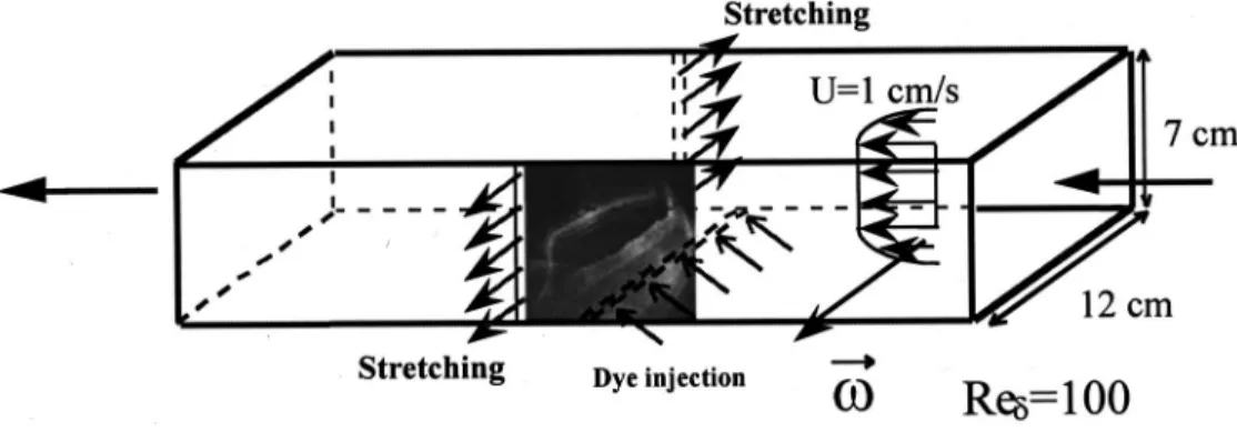
The purpose of this first part of the channel is to produce a well-controlled laminar flow. The second part of the chan-nel consists of a straight section 60 cm long 共Fig. 1兲. In the middle of this section, a slot is made in each lateral side and used to create a controlled suction of the main flow. At the end of this section, the flow is evacuated through a system which allows accurate measurement of the flow rate. In the first half of this straight section 共before the suction兲, the laminar flow creates a boundary layer on each side of the channel. Since the suction slots are located on the lateral walls, only the vorticity coming from the boundary layers on the upper and lower walls is stretched by the suction. This stretching is parallel to the initial vorticity. The flow rates of the suctions on each sides are identical, and can be measured and controlled. If the suction is constant at all slots, vortices are generated in phase on the upper wall and on the lower wall, and their vorticity is of opposite sign.33 Depending on the suction rate and on the flow rate of the main flow, these vortices interact, merge, or remain separate from each other or from the next pair of vortices generated on the same wall. In the experiments described in this paper, the suction is generated by a hole of 0.6 cm diameter on each lateral side located 0.5 cm up from the bottom of the channel 共Fig. 2兲.

The initial vorticity, stretched by these suctions, is enhanced and produces a vortex on the lower wall only. Below a cer-tain flow rate at the exit of the channel, the vortex remains stationary at this location,34sometimes with a low-amplitude precession. Above this flow rate, the vortex is elongated in the direction of the flow and may break up, in which case another one is generated in its place, and so on. In addition, in the experiments reported here a step of 1.1 cm high shown in Fig. 2 was placed just before the suction. This step pro-duces a more stable vortex with a smaller precessional mo-tion. In the following, x is the axis in the streamwise direc-tion, y is the vertical axis directed from the bottom to the top, and z is the spanwise axis parallel to the initial vorticity. 共0,0,0兲 is the origin at the bottom of the channel, in the stretching axis, and in the center as respect to the spanwise direction. The velocity component are (U,V,W), or (Ur,U␪,Uz) with respect to the center of the vortex. Q1 is

the downstream flowrate, Q2 is the flowrate through each

suction slot, the total incoming flow rate being Q₁⫹2Q₂.

III. ACOUSTIC EXPERIMENTAL TECHNIQUE

Our acoustic technique is based on the interaction be-tween an acoustic wave and the flow in the geometrical acoustics framework. Two 64 transducer arrays of 3.5 MHz central frequency are used. The size of each transducer is␭/2 关with ␭⫽0.42 mm) in width 共x direction on Fig. 1共a兲兴 and 10 mm in length 共z direction兲. Thus, the acoustic field is as-sumed to be bidimensional in the plane x⫺y 共perpendicular to the large size兲. Consequently, a plane wave is generated when all transducer of the array are emitting and a cylindri-cal wave when only one transducer is emitting.

The distance between two consecutive transducers is 0.42 mm. The transducer arrays can receive and emit. The electronic system which pilots the arrays can ‘‘time reverse’’ a wave 共see Sec. III B兲.

A. General context of the sound–flow interaction

The wavelength␭ of the ultrasonic wave at 3.5 MHz is 0.42 mm whereas the characteristic size d of the vortex core is around 5 mm so that the acoustic ray theory is valid (␭/dⰆ1).

Moreover, the characteristic flow velocity is around U

⬃10 cm/s. The Mach number is then M⫽U/c⬃10⫺4_,

where c is the speed of sound in the fluid at rest. Under these

FIG. 1. Experimental setup.

FIG. 2. Schematic view of the positions of the time-reversal mirrors in the channel共a兲 side view, 共b兲 top view.

conditions, the flow modifies locally the wave speed, leading to two effects to first order in M: an effect of deflection and an effect of acceleration.

The first effect is due to the vorticity ␻ of the flow which locally modifies the direction of the wave propagation,

n:dn/dt⫽␻丢n. If D is the distance between the two

trans-ducer arrays, the deflection produces a displacement ␦x be-tween the x location of the emitting transducer and the re-ceiving transducer which is of order of magnitude ␦x ⬃MD. In the experiment described in this paper, the chan-nel height is 7 cm and the distance D between the transducer arrays is 12 cm, leading to ␦x⬃10⫺2mm. The spatial reso-lution given by the array pitch being 0.42 mm, the refraction effect is expected to be negligible until about 40 time rever-sal processes 共see Sec. III C兲. For this reason, a straight-ray propagation is assumed in the following.

The second effect is due to the modification of the local wave speed v by the presence of the flow: v⫽c⫹u.n. The time shift of the acoustic signal after one crossing of the flow is given by␦t⬃ML/c, where L is the characteristic length of the flow. In our experiments, L corresponds to the vortex size d. The time shifts are inferred from Fourier transforms of the acoustic signals and the temporal resolution is fixed by the electronic noise level ␦t⬃10⫺9s, which allows a detection of fluid velocities above 10 cm/s.

It will be seen in the following that the onset of velocity detection is decreased when a time-reversal共TR兲 procedure is used. Finally, the analysis of the signal 共see Sec. III C兲 only includes the effect of acceleration of the ultrasound by the wave in the approximation of geometrical acoustics.

B. The time-reversal process

The acoustic technique is based on the interaction be-tween the sent ultrasound and the flow. However, because the effects of the flow on the ultrasonic wave are not strong enough, a time-reversal procedure is employed to artificially increase the velocity of the flow 共see Sec. III C兲 so that the effect of the flow becomes measurable. The analysis then consists in the reconstruction of the velocity field from the acoustic signal共see Sec. IV B兲.

Time-reversal invariance results from the invariance of the wave equation when changing the sign of the time. This invariance has been successfully verified in various media with scalar inhomogeneities, such as temperature or density gradients.35 A time-reversal procedure consists in sending a wave, for instance, a plane wave, through a medium by a transducer array, and to record the signal received by the second transducer array共see Fig 3兲. Then, ‘‘time reversing’’ the wave consists, for each transducer of the second array, in re-emitting the recorded signal after the sign of time has been changed, or, in other words, in emitting first the last part of the received signal. Since the medium is invariant under time reversal, the reversed wave lives again its anterior life until it recovers its initial shape of a plane wave, similarly to a movie seen backwards关Fig. 3共a兲兴.

Time-reversal invariance is broken as soon as the sound speed inhomogeneity depends on the direction of propaga-tion n, i.e., the inhomogeneity is vectorial rather scalar. This

is the case for the velocity of the flow. In such a case, the reversed wave does not recover its initial shape. Instead, the wave front deformation is amplified. In Fig. 3共b兲, this behav-ior is illustrated in the case of a vortex insonified by an initially plane wave. Heuristically, the acoustic rays forming the plane wave that cross the left part of the vortex are ac-celerated, they are the first to reach the receiving array. On the other side, the rays that cross the right side of the vortex are slowed down, they are the last to reach the array. In the TR procedure, the last received part of the signal, on the right side, is sent back first, and will cross a velocity field that, in this direction, speeds it up. Similarly, the first re-ceived part, on the left side, is the last to be sent back and will cross a velocity field that slows it down. Consequently, the distortion of the plane wave is increased by the TR procedure.36

Note that the whole system flow wave is time reversible. This has been experimentally checked by Roux.21In the ex-periments described in this paper, the violation of the time reversal invariance is obtained because the time is reversed for the wave and not for the flow.

C. Using time-reversal mirrors

We used the so-called double time-reversal mirrors 共double TRM兲 that has been described above 共two transduc-ers’ arrays located in front of each other on either side of the vortex as shown in Fig. 3兲. The TR procedure is repeated several times in order to significantly increase the effect of the flow on the wave.

The TRMs, arbitrarily numbered TRM1and TRM2关Fig.

3共b兲兴, send simultaneously a plane wave in opposite

direc-FIG. 3. Time-reversal experiment共a兲 for a medium with a scalar inhomo-geneity共time-reversal invariance兲 and 共b兲 in the presence of a vortex 共break-ing of time reversal invariance兲.

tions. S12(x) is the signal received by TRM2when TRM1 is

the emitter and S21(x) is the signal received by TRM1when

TRM2 is the emitter共x indicates the transducer position on

the arrays兲. These acoustic signals are then time reversed and simultaneously sent back by the two TRMs, and so on.

A phase shift⌬␾(x) is built as follows:

A first ‘‘blank’’ experiment is performed in order to measure the times-of-flight t₁₂0 and t₂₁0 in absence of flow. Indeed, in a fluid at rest, the acoustic wave is supposed to remain plane after several trips between the TRMs. How-ever, due to the finite aperture of the transducer arrays, the wave fronts are distorted by diffraction effects.36Those ref-erence times-of-flight t₁₂0 and t₂₁0 are then subtracted to t12

and t21 measured in the presence of a vortex, yielding the

time-shifts␦t12 and␦t21.

The time-shifts ␦t12 and␦t21 not only account for the

effect of the fluid motion but also for possible effects of the temperature or density inhomogeneities which modify the local speed of sound. However, these last effects do not de-pend on the direction of the acoustic propagation and cancel out in the difference ␦t12⫺␦t21.

12,13

Note here that ␦t12

⫹␦t21 allows to measure the temperature or concentration

gradients without being perturbed by the flow velocity. The phase shift is defined as: ⌬␾(x)⫽␻关␦t₂₁(x) ⫺␦t₁₂(x)兴/2. The dependence of ⌬␾(x) on the velocity field

u(r) is given by ⌬␾共x兲⫽␻₂

冉

冕

冕

冊

冉

冕

冕

冊

which, at the first order in M, reduces to ⌬␾共x兲⯝_c␻2

冕

TRM₁ TRM₂

u.nd y . 共3.2兲

It has been shown in previous works23 that the phase shift⌬␾N(x) increases linearly with the number N of itera-tions whereas noise only increases as the square root of N. Consequently, the signal-to-noise ratio is enhanced by time reversal. A typical phase shift ⌬␾_N(x)/N is shown in Fig. 5共a兲 for N⫽5 time-reversal processes.

IV. VORTEX CHARACTERIZATION

In the experiments described in this section, the flowrate of the suction Q2is fixed, equal to 6.2

l

down-stream flow rate Q1 is the control parameter. For small

val-ues of Q1, the vortex remains almost stationary, located near

the small step. Above a threshold Q1c⫽8.7

l

vor-tex goes unstable: it is advected with the main flow until a critical distance from the step where it breaks down. This behavior leads to periodic cycles of birth 共vortex formation near the step兲, advection and breakdown. In this section, ex-amples of results obtained with the double time-reversal mir-rors are presented when the flow rate Q1is below the

thresh-old Q1c. The next section deals with results in the unstable

regime of cycles.

A. Study of the precession motion

For Q1⬍Q1c, the vortex remains near the step.

How-ever, a small precession motion can be observed, which am-plitude increases when the flowrate Q1 is increased. The

double TRMs allows to follow easily this motion. Indeed, the zero value in the phase shift⌬␾(x0)⫽0 corresponds to a ray

which crosses the center x0 of the vortex. Figure 4共a兲 shows

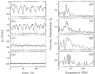
the temporal variation of x0for different flowrates Q1. It can

be seen that the precession amplitude increases with Q₁. Figures 4共b兲 shows the corresponding Fourier transforms. The frequency is of order 0.1 Hz and does not seem to de-pend significantly on the flowrate.

Experiments are in progress in order to characterize the precession as a function of the stretching. In the following, only vortices with a very slow and low amplitude precession will be presented for the velocity reconstruction.

B. Velocity field reconstruction

As already mentioned, the vortex can be considered as stationary for flowrates small enough. In this case, a recon-struction method to access the velocity field from the phase shift has been developed. An example of phase distortion is shown on Fig. 6共a兲 for Q1⫽1.3

l

ob-tained from an average on 200 samples on the same vortex. Let us recall that the effect of the velocity is integrated along the acoustic rays on the y direction 共sound propagation di-rection兲, so that it is not possible to get the y dependence of the velocity u( y ). On the x direction, on the contrary, u(x) is obtained with a spatial resolution given by the array pitch 共0.42 mm兲. In the case of an axisymmetric vortex, this re-striction has no consequence thanks to the invariance be-tween x and y. This case has been investigated in a previous study.23

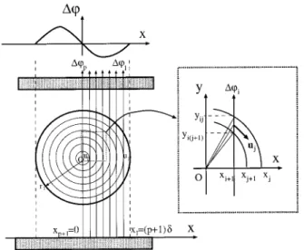
The axisymmetric reconstruction algorithm consists in dividing the propagation area into p small concentric rings r苸关ri⫹1,ri兴 of size corresponding to the distance between

FIG. 4. Study of the precession motion: time series of the x0position共center

of the vortex兲 for Q2⫽6.2l /min and 共a兲 Q1⫽8.4l /min, 共b兲 Q1

⫽7.2l /min, 共c兲 Q1⫽5.1l /min, 共d兲 Q1⫽3.0l /min共the position of the

suction hole is x⫽⫺35 mm). Graphs 共e兲, 共f兲, 共g兲, and 共h兲 are the corre-sponding normalized Fourier transforms.

two transducers. The orthoradial velocity u_␪ is sampled in each ring and takes the values ui 共see Fig. 5兲.

r1 is the edge of the vortex, defined as the first point

共coming from outside the vortex兲 where the phase shift ⌬␾(x) is not zero. rp⫹1is the center of the vortex, where the phase shift is also zero 关all the velocities u_␪(r) are perpen-dicular to the ray direction that crosses the vortex center兴, and p⫹2 is the number of experimental data points. The phase distortion ⌬␾i⫽⌬␾(xi⫹1) are sampled at the trans-ducer position xi⫹1.

In the first ring r1, the velocity u1 is deduced from the

experimental phase shift ⌬␾1 by a relation resulting from

Eq. 共3.1兲: ⌬␾1⫽2␻/c2r2ln((

冑

2 2_⫹r

1)/r2)u1. Then, in

the second ring r2, the velocity u2 can be obtained from

⌬␾2 and the velocity u1 previously calculated at the

previ-ous step: ⌬␾2⫽2␻/c2兵r2ln关(

冑

冑

冑

2)/r3兴u2其. This process is

re-peated until the center of the vortex is reached using the general relation: ⌬␾i⫽Mi juj, 共4.1兲 where Mi j⫽ 2␻ c2 rj⫹1ln

冑

冑

M is an invertible, triangular matrix. Thus, u can be reconstructed from the measurements of⌬␾.

This assumes that the vortex is axisymmetric, which is not exactly the case in our experiment. Indeed, the vortex has a slightly elliptical shape. It can be seen in Fig. 2 that, far from the vortex core, the shape is clearly non axisymmetric and, from these external contours, should rather be called elliptical. However, closer to the core, the streamlines be-come circular. Actually, visualizations only give a qualitative idea of the vortex shape but carry no information on the velocity distribution.

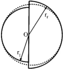
In this case, a possible way to obtain a bidimensional reconstruction is to make an assumption on the vortex shape coming from visualizations for instance. We chose an alter-native solution by mixing two axisymmetric reconstructions for both half parts of the phase distortion: ␾r 共right兲 for the negative phase distortion (n_r elements兲 and␾_l 共left兲 for the positive phase distortion (n_l elements, with n_r⫹n_l⫽64 transducers兲. The velocity profiles u_r and u_l are indepen-dently obtained by inverting the M_l and M_r. A typical phase distortion is shown in Fig. 6共a兲 and the corresponding reconstructed half profiles urand ulon solid line in Fig. 6共b兲 for Q1⫽1.3

l

can be seen that the right part is 18 mm long whereas the left part is 12 mm long. An elliptical shape is used to correct this discontinuity and to approach the real shape of the vortex 共see Fig. 7兲. The values of the velocity are then corrected with the help of this new shape关curve in dashed line on Fig. 6共b兲兴.

FIG. 5. Reconstruction principle for a circular vortex shape: in each ring, the velocity is taken constant and extracted from the phase profile 关Eqs. 共4.1兲 and 共4.2兲兴.

FIG. 6. 共a兲 Phase distortion as a function of the transducer position x for Q1⫽1.3l /min and Q2⫽6.2l /min.共b兲 Reconstructed orthoradial velocity as a

function of the radius r.

V. ACCESSING THE VORTEX DYNAMICS A. Determination of the vortex characteristics

The relevant characteristics of the vortex are the diam-eter of the vortex and its circulation, or its diamdiam-eter and its maximum velocity.

Let rmbe the radius where the velocity is maximum and takes the value Um, and xmthe transducer position where the phase shift is maximum and takes the value ⌬␾m.

⌬␾(x) and U(r) can be written: ⌬␾共x兲⫽⌬␾mf共x˜,Re,Restretching兲,

共5.1兲 u共r兲⫽Umg共r˜,Re,Restretching兲,

where x˜⫽x/rm and r˜⫽r/rm 共so that y˜⫽y/rm), Re is the Reynolds number of the mean flow and Restretchingis the

Rey-nolds number based on the stretching velocity and the diam-eter of the hole through which the stretching is produced.

If the distance between the two transducer arrays is large enough, the phase shift can be written:

⌬␾共x兲⫽_c␻2

冕

冕

This relation implies that the ratio⌬␾m/rmUm depends only on the two Reynolds numbers共Re and Restretching). The

circulation ⌫⫽兰cu(r).dr⬃2␲rmUm is then obtained only from the measurement of⌬␾m by the relation:

⌫⫽⌬␾mF共Re,Restretching兲. 共5.4兲

The diameter of the vortex 2rmcan be deduced from the measurement of xmusing the same relations and the fact that the position x1 of the zero phase shift corresponds to the

radius r1 where the velocity is also zero共see Fig. 5兲:

rm⫽xmG共Re,Restretching兲. 共5.5兲

Thus, it is sufficient for the characterization of the vortex to extract only xmand⌬␾mfrom the phase shift profile. The

FIG. 8. Temporal evolution of共a兲 x0, location of the center of the vortex, 共b兲 rm, the vortex radius, and共c兲 ⌫, the circulation of the vortex for four

consecutive cycles.共d兲, 共e兲, and 共f兲 show the average evolution of these parameters on 20 cycles. Q1⫽14l /min, Q2⫽6.2l/min.

FIG. 7. From the two circular reconstructions to the elliptical shape closer to the real vortex.

functions F and G have to be calculated only once for each given flowrate and stretching. If the vortex is not symmetric, an average value is taken.

B. Example of vortex dynamics

The instantaneous phase distortion is recorded as a func-tion of time. F and G are deduced from the first profile. Then, x0, xm, and ⌬␾m are extracted at each step and rm and⌫ are calculated.

Figure 8 shows the temporal evolution of these charac-teristics on a few periods of formation, advection and break-down of a vortex.

In Figs. 8共d兲, 8共e兲, and 8共f兲, these characteristics have been plotted on a mean cycle 共averaging over 20 cycles兲.

It can be seen that the vortex size remains roughly con-stant while the circulation increases until a maximum value before the vortex breaks down. The vortex is first advected with a constant velocity then slows down a little bit before it breaks.

C. Bidimensional tracking using cylindrical waves

The previous study was performed using plane waves. This was done for various reasons: the signal amplitude is higher because all the transducers are used, and the signal-to-noise ratio is better because time reversal process can be used.

However, we have seen that the vortex tracking using plane waves is only possible in one direction: the x direction along the chanel. In order to get the trajectory of the vortex in the x-y plane, another process using cylindrical waves has been developed. In that case, the time reversal process can-not be used any longer: the only effect of a time-reversal procedure would be the defocalization of the reversed wave without increasing the signal-to-noise ratio.36

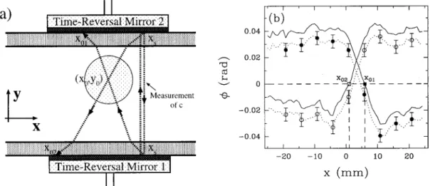
Only one transducer on each array emits. The sources are located in front of each other 关same position xs on the arrays, see Fig. 9共a兲兴. The received signals on both arrays are written as

FIG. 9.共a兲 Schematic view of acoustic ray trajectories in the case of cylindrical waves. The xs-xsrays are used to measure the sound speed. The xs-x01and

xs-x02rays are used to locate the center (x0,y0) of the vortex.共b兲 The experimental phase distortions␾12(x) and␾21(x) are plotted as a function of x in

dashed lines. The solid lines represent the phase shift␾v,12(x) and␾v,21(x) related to the vortex only, without the contribution of the propagation term. The

x positions x01and x02, where␾v,12and␾v,21vanish allow to deduce the position (x0,y0) of the vortex center. Q1⫽12.4l /min, Q2⫽6.2l/min.

FIG. 10. Temporal evolution of the position 共a兲 x0 and 共b兲 y0 of the center of the vortex for 6 different cycles where Q1⫽12.4l /min and Q2

⫽6.2l /min.

␾共␪兲⫽_c⫹U␻L meancos␪ ⫺␻ c2

冕

冕

where Umeanis the mean velocity in the chanel共constructed

with Q1), ␪ is the angle (Umean,n) and L is the distance

between emitter and receiver: L⫽D/sin␪ 共see Fig. 9兲. In the case of plane waves described before,␪⫽␲/2 so that the dependence of ␾ with Umean cancels out. On the

other hand, the reverse signal allows to eliminate the first term ␻L/c by subtracting the direct and reverse signals共see Sec. III C兲.

In the case of cylindrical waves, c has to be determined. For this, we use the direct ␾12 and reverse ␾21 signals as

described in Fig. 9: c⫽2␻D/(␾12⫹␾12). The second term

␻LUmeancos␪/c2 is much smaller that the others in our

ex-periment and can be neglected, mainly because ␪ remains close to ␲/2: ␻LUmeancos␪/c2⬃10⫺3rad, whereas

(␻/c2)兰₀Lu(r).ndl is of order 10⫺2rad.

The experimental phase distortions ␾12(x) and ␾21(x)

are plotted in Fig. 9 in dashed lines. The solid lines represent ␾v(x)⫽␾(x)⫺␻L/c⬃␻/c2兰0

L

u(r).ndl which is the phase

shift related to the vortex only.

The transformation between x and ␪ includes the effect of refraction on the interface Plexiglas/water. The positions x01 and x02 where ␾v,12(x) and␾v,21(x) vanish define two

acoustic rays crossing the vortex center. From xs, x01 and

x02, we first compute the angles ␪1 and ␪2 between the y

axis and the direction of propagation n corresponding to those two rays by solving for ␪_iin

x_0i⫺x_s⫽D tan␪_i⫹2d tan

冋

冉

sin␪_i

冊册

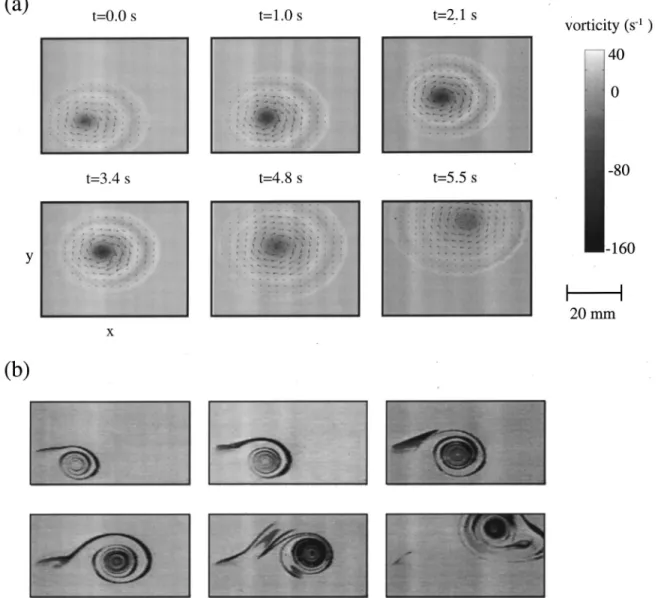
FIG. 11. 共a兲 Sequence of pictures showing the vorticity field 共gray level兲, the velocity field 共arrays兲 and the motion of the vortex. The vorticity and velocity are deduced from the maximum phase shift in the case of plane waves, so that the values are taken with an arbitrary scale.共b兲 Sequence of experimental pictures: the vortex is visualized with fluorescent dye.

where n_w and n_p are, respectively, the acoustic refractive indices of water and Plexiglas 共with n_w⫽2.7 and n_p⫽1.5), and d is the Plexiglas width. The coordinates (x0,y0) of the

vortex center are then given by the intersection of the two rays: x₀⫽1 2

冉

冊

冉

冊

The values are plotted in Fig. 10 as a function of time for six cycles of a same experiment. The evolution of the differ-ent cycles are similar even if they do not superimpose. Fig-ure 11 shows the position, the vorticity and the velocity fields at different times along a cycle.

VI. CONCLUSION

The acoustic technique presented in this paper has been applied for the first time to the study of the vortex structure and dynamics. The measured phase distortion gives directly the circulation. In the case of a vortex, the velocity field can be deduced with a good accuracy. The measurement is glo-bal and non intrusive. It allows the access to the whole vor-tex dynamics.

The results presented here prove that this technique is relevant for the study of vortices and adds to classical tech-niques such as laser doppler velocimetry, particles image ve-locimetry, hot wire, etc.

Most of the other nonintrusive experimental techniques need the injection of particles. The measured velocity is then the velocity of the particles which is not always the flow velocity. It has been shown by Wunenburger et al.5that, in the particular case of vortex flows, the measurements can be biased by the particles demixion. In the case of turbulent flows, the use of particules can be more irrevelant because of the complex behavior of the particles in such a flow.

Acoustical measurements based on flow-wave interac-tion 共without particles兲 are used by Baudet et al.37 for the study of turbulent flows. They show that acoustic measure-ments directly obtained in the Fourier space give access to the spatial scales of the flow 共without localization of the structures兲. Work is in progress to use this time-scale acous-tic interferometry technique on vortex breakdown.

ACKNOWLEDGMENTS

We would like to thank Eduardo Wesfreid and Claire Prada for fruitful discussions.

1

O. Cadot, S. Douady, and Y. Couder, ‘‘Characterization of the low-pressure filaments in a three-dimensional turbulent shear flow,’’ Phys. Fluids 7, 630共1995兲.

2_{E. D. Siggia, ‘‘Numerical study of small-scale intermittency in} three-dimensional turbulence,’’ J. Fluid Mech. 107, 375共1991兲.

3_{M. E. Brachet, ‘‘Direct simulations of three-dimensional turbulence in the} Taylor-Green vortex,’’ Fluid Dyn. Res. 8, 1共1991兲.

4_{J. Jimenez, A. A. Wray, P. G. Saffman, and S. Rogallo, ‘‘The structure of} instense vorticity in isotropic turbulence,’’ J. Fluid Mech. 255, 65共1993兲. 5_{R. Wunenburger, B. Andreotti, and P. Petitjeans, ‘‘Influence of precession} on velocity measurements in a strong laboratory vortex,’’ Exp. Fluids 26

共1999兲.

6_{P. Petitjeans, J. H. Robres, J. E. Wesfreid, and N. Kevlahan,} ‘‘Experimen-tal evidence for a new type of stretched vortex,’’ Eur. J. Mech. B/Fluids

17, 549共1998兲.

7_{P. R. Gromov, A. B. Ezerskii, and A. L. Fabrikant, ‘‘Sound scattering by} a vortex wake behind a cylinder,’’ Sov. Phys. Acoust. 28, 552共1982兲. 8_{A. L. Fabrikant, ‘‘Sound scattering by vortex flows,’’ Sov. Phys. Acoust.}

29, 152共1983兲.

9

P. V. Sakov, ‘‘Sound scattering by a vortex filament,’’ Acoust. Phys. 39, 280共1993兲.

10_{D. W. Schmidt and P. L. Tilman, ‘‘Experimental study of sound wave} phase fluctuations caused by turbulent wakes,’’ J. Acoust. Soc. Am. 47, 1310共1970兲.

11_{R. H. Engler, D. W. Schmidt, W. Wagner, and B. Weitemeier,} ‘‘Nondis-turbing acoustical measurement of flow fields; new developments and ap-plications,’’ J. Acoust. Soc. Am. 85, 72共1989兲.

12

K. B. Winters and D. Rouseff, ‘‘Tomographic reconstruction of stratified fluid flow,’’ IEEE Trans. Ultrason. Ferroelectr. Freq. Control 40, 26

共1993兲.

13

S. A. Johnson, J. F. Greenleaf, M. Tanaka, and G. Flandro, ‘‘Reconstruct-ing three-dimensional temperature and fluid velocity vector fields from acoustic transmission measurements,’’ ISA Trans. 16, 3共1997兲. 14

F. Lund and C. Rojas, ‘‘Ultrasound as a probe of turbulence,’’ Physica D

37, 508共1989兲.

15_{H. Contreras and F. Lund, ‘‘Ultrasound as a probe of turbulence. II,} Tem-perature inhomogeneities,’’ Phys. Lett. B 149, 127共1990兲.

16_{R. Berthet and F. Lund, ‘‘The forward scattering of sound by vorticity,’’} Phys. Fluids 7, 2522共1995兲.

17_{C. Baudet, S. Ciliberto, and J. F. Pinton, ‘‘Spectral analysis of the Von} Ka´rma´n flow using ultrasound scattering,’’ Phys. Rev. Lett. 67, 193

共1991兲.

18

J. F. Pinton, C. Laroche, S. Fauve, and C. Baudet, ‘‘Ultrasound scattering by buoyancy driven flows,’’ J. Phys. II 3, 767共1993兲.

19_{F. Vivanco and F. Melo, ‘‘Surface waves scattering by a vertical vortex,’’} Nonlinear Dynamics and Acoustics, ETSEIB, 1998, pp. 114–122. 20

M. Oljaca, X. Gu, A. Glezer, M. Baffico, and F. Lund, ‘‘Ultrasound scat-tering by a swirling jet,’’ Phys. Fluids 10, 886共1998兲.

21_{P. Roux and M. Fink, ‘‘Experimental evidence in acoustics of the} viola-tion of time-reversal invariance induced by vorticity,’’ Europhys. Lett. 32, 25共1995兲.

22

P. Roux, J. de Rosny, M. Tanter, and M. Fink, ‘‘The Aharonov-Bohm effect revisited by an acoustic time-reversal mirror,’’ Phys. Rev. Lett. 79, 3170共1997兲.

23_{S. Manneville, A. Maurel, P. Roux, and M. Fink, ‘‘Characterization of a} large vortex using acoustic time-reversal mirrors,’’ Eur. Phys. J. B 共un-published兲.

24_{M. Baffico, D. Boyer, and F. Lund, ‘‘Propagation of acoustic waves} through a system of many vortex rings,’’ Phys. Rev. Lett. 80, 2590共1998兲. 25_{D. Boyer and F. Lund, ‘‘Propagation of acoustics waves in disordered}

flows composed of many vortices’’共unpublished兲.

26_{V. E. Ostashev, ‘‘Acoustics in moving inhomogeneous media,’’ edited by} E. & FN SPON, London, ISBN 0 419 22430 0共1997兲.

27_{A. Petrossian and J. F. Pinton, ‘‘Sound scattering on a turbulent, weakly} heated jet,’’ J. Phys. II 7, 801共1997兲.

28

R. Labbe´ and J. F. Pinton, ‘‘Propagation of sound through a turbulent vortex,’’ Phys. Rev. Lett. 81, 1413共1998兲.

29_{B. Dernoncourt, J. F. Pinton, and S. Fauve, ‘‘Experimental study of} vor-ticity filaments in turbulent swirling flows,’’ Physica D 117, 181共1998兲. 30

B. Lipkens and P. Blanc-Benon, ‘‘Propagation of finite amplitude sound through turbulence: a geometric acoustics approach,’’ C. R. Acad. Sci., Ser. IIb: Mec., Phys., Chim., Astron. 320, 477共1995兲.

31_{P. Chevret, P. Blanc-Benon, and D. Juve´, ‘‘A numerical model for sound} propagation through a turbulent atmosphere near the ground,’’ J. Acoust. Soc. Am. 100, 3587共1996兲.

32_{V. E. Ostashev, P. Blanc-Benon, and D. Juve´, ‘‘Coherent function of a} spherical acoustic wave after passing through a turbulent jet,’’ C. R. Acad. Sci., Ser. IIb: Mec., Phys., Chim., Astron. 326, 39共1998兲.

33

P. Petitjeans, J. E. Wesfreid, and J. C. Attiach, ‘‘Vortex stretching in a

laminar boundary layer flow,’’ Exp. Fluids 22, 351共1997兲. 34

P. Petitjeans and J. E. Wesfreid, ‘‘Vortex stretching and filaments,’’ Appl. Sci. Res. 57, 279共1997兲.

35_{M. Fink, ‘‘Time-reserved acoustics,’’ Phys. Today 50, 34共1997兲.} 36_{P. Roux, ‘‘Applications des miroirs acoustiques a` retournement temporel a`}

la focalisation dans un guide d’onde et a` la caracte´risation d’e´coulements hydrodynamiques,’’ Ph.D. thesis, University of Paris VI, 1996. 37_{C. Baudet, O. Michel, and W. J. Williams, ‘‘Detection of coherent}

vortic-ity structures using time-scale resolved acoustic spectroscopy,’’ Physica D