Dealing with uncertainty : a comparison of robust optimization and partially observable Markov decision processes

Dealing with Uncertainty: A Comparison of Robust Optimization and Partially Observable Markov Decision Processes

by

Casey Vi Horgan

B.S., Mathematics US Air Force Academy (2012)

Submitted to the Department of Aeronautics and Astronautics in partial fulfillment of the requirements for the degree of

Master of Science in Aeronautics and Astronautics at the

MASSACHUSETTS INSTITUTE OF TECHNOLOGY June 2014

MASSACHUSETTS INSTITTE OF TECHNOLOGY

LIBRARIES

The author hereby grants to MIT and The Charles Stark Draper Laboratory, Inc. permission to reproduce and to distribute publicly paper and electronic copies of this thesis

document in whole or in part in any medium now known or hereafter created.

A u th or ... De

C ertified by ...

Signature redacted

AMay 22, 2014

Signature redacted

..

(//ichael J. Ricard Distinguished Member of the Technical Staff, Charles Stark Draper Laboratory, Inc. Tjiesis Supervisor

Certified by...

....

Signature redacted

Leslie P. Kaelbling Professor of Computer Science and Engineering Thesis Supervisor C ertified by ...

A ccepted by ...

Signature redacted

Signature redacted

Paulo C. Lozano Associate Professor of Aeronautics and Astronautics

Dealing with Uncertainty: A Comparison of Robust Optimization

and Partially Observable Markov Decision Processes

by

Casey Vi Horgan

Submitted to the Department of Aeronautics and Astronautics on May 22, 2014, in partial fulfillment of the

requirements for the degree of

Master of Science in Aeronautics and Astronautics

Abstract

Uncertainty is often present in real-life problems. Deciding how to deal with this uncertainty can be difficult. The proper formulation of a problem can be the larger part of the work required to solve it. This thesis is intended to be used by a decision maker to determine how best to formulate a problem. Robust optimization and partially observable Markov decision processes (POMDPs) are two methods of dealing with uncertainty in real life problems. Robust optimization is used primarily in operations research, while engineers will be more familiar with POMDPs. For a decision maker who is unfamiliar with one or both of these methods, this thesis will provide insight into a different way of problem solving in the presence of uncertainty. The formulation of each method is explained in detail, and the theory of common solution methods is presented. In addition, several examples are given for each method. While a decision maker may try to solve an entire problem using one method, sometimes there are natural partitions to a problem that encourage using multiple solution methods. In this thesis, one such problem is presented, a military planing problem consisting of two parts. The first part is best solved with POMDPs and the second with robust optimization. The reasoning behind this partition is explained and the formulation of each part is presented. Finally, a discussion of the problem types suitable for each method, including multiple applications, is provided.

Thesis Supervisor: Michael J. Ricard

Title: Distinguished Member of the Technical Staff, Charles Stark Draper Laboratory, Inc.

Thesis Supervisor: Leslie P. Kaelbling

Acknowledgments

First and foremost, I have to thank my amazing family for all of their love and support over the past two years. I know that I would not be here today if I did not have them. My wonderful roommate also made my time here very enjoyable. Meghan, you have been such a great roommate and have made our apartment a place where I enjoy spending my time. The value of that cannot be emphasized enough.

I must thank Draper Lab for giving me the opportunity to attend MIT. This thesis was prepared at Charles Stark Draper Laboratory, Inc. under Internal Research and Develop-ment funding number 29484-001. I especially want to thank my advisor, Dr. Michael Ricard. He has provided constant support and encouragement beyond the duties of a thesis super-visor. His dedication to his students and his community is inspiring.

I am thankful for the support of my MIT thesis supervisor, Professor Leslie P. Kaelbling.

Thank you for your help and expertise. I appreciate your flexibility and willingness to be my supervisor. Professor Frazzoli, thank you for overseeing my academics at MIT. I appreciate your support despite the long distance.

Finally, I would like to thank those who made the hours in the office not only bearable, but enjoyable. Amy, Matt, Will, and Rob, you are all awesome! I cannot imagine days at Draper without you.

The views expressed in this thesis are those of the author and do not reflect the official policy or position of the United States Air Force, Department of Defense, or the U.S.

Contents

3 Partially Observable Markov Decision Processes 3.1 Markov Decision Processes . . . .

17 17 18 18 21 . . . . 2 1 . . . . 23 . . . . 23 . . . . 25 . . . . 25 . . . . 26 . . . . 28 . . . . 35 . . . . 38 . . . . 40 . . . . 43 45 45

3.2 MDP Example ... 46

3.3 MDP Solution Methods . . . . 51

3.3.1 Value Iteration . . . . 51

3.3.2 Policy Iteration . . . . 56

3.3.3 Linear Programming . . . . 57

3.4 Partially Observable Markov Decision Processes . . . . 61

3.5 Tiger Problem . . . . 62

3.6 POMDP Solution Algorithms . . . . 65

3.6.1 Policy Trees . . . . 65

3.6.2 Adjusted Value Iteration Algorithm . . . . 67

3.6.3 Infinite Horizon . . . . 72

3.6.4 Incremental Pruning . . . . 74

3.7 Rock Sample Problem . . . . 77

3.8 Summary . . . . 83

4 Military Planning Problem 85 4.1 The Scenario . . . . 85

4.2 The POMDP Problem . . . . 87

4.2.1 POMDP Results . . . . 93

4.3 The RO Problem . . . . 96

4.3.1 The Linear Program Formulation . . . . 96

4.3.2 The Robust Optimization Formulation . . . 101

5 Comparison of the Methods 111 5.1 POMDP Reformulated as a Linear Program . . . 111

5.2 RO Reformulated as an MDP . . . 114

5.4 Robust Optimization Applications . . . 117

5.4.1 Transport Problems. . . . 118

5.4.2 Scheduling Problems . . . 119

5.4.3 M ixing Problems . . . 121

5.4.4 Com mon Features . . . 122

5.5 POM DP Applications . . . 123

5.5.1 Airplane Identification . . . . 123

5.5.2 W eapon Allocation . . . . 124

5.5.3 Robot Navigation . . . . 125

5.5.4 Com mon Features. . . . . 126

6 Conclusion 127 6.1 Sum m ary . . . . 127

List of Figures

2-1 Movement of Optimal Solution . . .

2-2 Variation of Objective Function . . .

2-3 Varying Objective Functions . . . . . 2-4 Original and Worst Case Constraints

3-1 Rock Sample Problem Environment

3-2 Rock Sample States . . . .

3-3 Horizon 1 Policy Trees . . . . 3-4 Horizon 2 Policy Trees . . . .

3-5 Horizon 1 a-Vectors . . . . 3-6 Horizon 2 a-Vectors . . . . 3-7 Horizon 3 a-Vectors . . . . 3-8 Horizon 4 a-Vectors . . . . 3-9 Horizon 49 a-Vectors . . . . 3-10 Horizon 50 a-Vectors . . . . 3-11 Infinite Horizon a-Vectors . . . .

3-12 Infinite Horizon Grid Position 1 . . .

3-13 Infinite Horizon Grid Position 2 . . .

3-14 Infinite Horizon Grid Position 3 . . .

32 36 37 40 47 . . . . 4 7 . . . . 6 6 . . . . 6 6 . . . . 6 8 . . . . 6 9 . . . . 7 1 . . . . 7 1 . . . . 7 2 . . . . 7 3 . . . . 7 4 . . . . 8 1 . . . . 8 2 . . . . 8 2

List of Tables

2.1 Factory Information . . . . 2.2 Chair Coefficient Uncertainty 2.3 Objective Function Uncertainty 2.4 Constraint Limit Uncertainty 2.5 Multiple Uncertainties . . . . . . . . 22 . . . 31 . . . 36 . . . 39 42 3.1 Rock Sample States . . . . 47

3.2 Move Left Transition Matrix . . . . 48

3.3 Move Right Transition Matrix . . . . 48

3.4 Collect Transition Matrix . . . . 49

3.5 Move Right Rewards . . . . 49

3.6 Move Left Rewards . . . . 49

3.7 Collect Rewards . . . . 50

3.8 Optimal State Transitions . . . . 51

3.9 Rock Sample Problem Value Iteration . . . . 55

3.10 Rock Sample Problem Value Iteration Policy . . . . 55

3.11 Optimal Policy . . . . 60

3.12 POMDP Components . . . . 62

3.13 Open Left Transition Matrix . . . . 63

3.15 Listen Transition Matrix 3.16 3.17 3.18 3.19 3.20 3.21 3.22 3.23 3.24 3.25 3.26 3.27 4.1 4.2 4.3 4.4 4.5 4.6 4.7 4.8 4.9 4.10 4.11 4.12

Train Transition Probabilities . . . . Inspect Transition Probabilities . . . . Declare Deployable Transition Probabilities. . Train Observation Probabilities . . . . Inspect Observation Probabilities . . . . Declare Deployable Observation Probabilities . Rew ards . . . . POMDP Example . . . . Linear Program Components . . . . Linear Program Variables . . . . Squadron Distribution . . . . Allocation Weights . . . . Open Left Observations

Open Right Observations. Listen Observations . . . .

Open Left Rewards . . . .

Open Right Rewards . . . Listen Rewards . . . . Check Transition Matrix . Check Rewards . . . . Move Right Observations Move Left Observations Collect Observations . . . Check Observations . . . . . . . . 63 . . . . 63 . . . . 64 . . . . 64 . . . . 64 . . . . 64 . . . . 78 . . . . 78 . . . . 79 . . . . 79 . . . . 79 . . . . 80 91 91 91 92 92 92 93 93 97 97 99 99 63

4.13 Task Weights ... ... 100

4.14 Resource Requirements . . . 100

4.15 LP Solution . . . 101

4.16 Robust Optimization Components . . . . 102

4.17 RO Variables . . . . 103

4.18 Task Weight Deviation . . . . 104

4.19 Allocation Weight Deviation . . . 104

4.20 Resource Requirement Deviation . . . 105

4.21 Robust Examples . . . 105

4.22 More Robust Examples . . . 106

4.23 Additional Task Constraints . . . 108

4.24 Additional Squadron Constraints . . . 108

Chapter 1

Introduction

1.1

Motivation

Real-world problems are subject to the uncertainties of life. The best way to deal with that uncertainty is often unclear. Various formal methods exist for decision making in the presence uncertainty, but their applicability differs greatly based on the structure of the problem. This thesis will examine two methods, robust optimization and partially observable Markov decision processes (POMDPs). An examination of the strengths of these methods will be provided, along with analysis designed to help a decision maker determine which is more suited to the problem at hand. Robust optimization is common in operations research, while POMDPs are prevalent in other engineering disciplines. When faced with uncertainty, researchers in each of these fields often reach for the method which is most familiar, then manipulate their problems into a form solvable by that method. This can sometimes work, but applying a different method could produce significantly better results. This thesis aims to give the decision maker familiarity with robust optimization and POMDPs, providing more flexibility in problem formulation.

1.2

Overview

The main body of this thesis is divided into four chapters. Chapter 2 provides a thorough overview of robust optimization (RO). This chapter first outlines several robust optimization techniques. Then, a detailed explanation of cardinality-constrained robust optimization is provided. This is followed by a fully worked example with a comparison of the RO solution to the nominal solution to the linear program (LP). In this example, RO is applied to several different types of uncertainty.

Chapter 3 is a detailed description of Markov decision processes (MDPs) and POMDPs. It includes an explanation of three solution methods for MDPs: value iteration, policy iter-ation, and linear programming. It then covers policy trees and POMDP solution methods, including incremental pruning. Several examples are provided.

Chapter 4 outlines a military planning problem that incorporates both robust optimiza-tion and POMDPs. Half of the problem is solved using POMDPs, while the other half is solved using RO. The differences in problem structure between the two parts-and how this impacts which method is used to solve each part-is discussed.

Chapter 5 analyzes the problem types to which each method is best suited. The problem from Chapter 4 is revisited, attempting to solve each part of the problem with the opposite method from Chapter 4. The resulting difficulties lead to a discussion of the differences in the purpose of each method. The sources of uncertainty in RO and POMDPs are examined. Finally, several applications of each method are discussed.

1.3

Contributions

This thesis provides a thorough examination of both robust optimization and POMDPs. Little work has been done comparing the problem formulations for these two methods. This thesis can serve as a guide for the decision maker, helping to determine which method is

best for a given problem structure. This thesis gives an in-depth look at the structure of each formulation, including the types of uncertainty each can handle. Additional comparison shows that the two methods are fundamentally different in the problem types they can solve.

Chapter 2

Robust Optimization

Linear programming is a useful tool for solving well-defined problems, allowing for efficient optimal solutions to an objective function and an unambiguous set of constraints. Unfortu-nately, we rarely have such precise data in real-world problems. Many details of a problem may be subject to uncertainty. While linear programming is good for precise problems, it is not equipped to handle potential variation. This is the domain of robust optimization. In this chapter, a linear programming problem will be presented as the driving example. Then, the theory of robust optimization will be discussed before the method is applied to the example problem.

2.1

Example Problem

Consider a furniture factory that makes tables and chairs. Each table requires a specific number of man-hours in carpentry and painting. The same is true for the chairs. The factory has limits on the available man hours of each type (carpentry and painting). The goal of the factory, of course, is to maximize profit, subject to the available labor constraints. Table 2.1 contains the factory information.

Tables Chairs Hours Available

Profit $6 $5

Carpentry 4 hrs 5 hrs 3000 Painting 3 hrs 2 hrs 1700

Table 2.1: Factory Information

That results in the following linear program:

max 6t

+

subject to 4t + 5c < 3000

3t + 2c < 1700

t c > 0

The objective function, 6t + 5c, represents the factory's profit, $6 for every table and $5 dollars for every chair produced. The goal is to maximize this profit. The first two constraints ensure that the factory's labor limitations are not exceeded. Finally, the number of tables and chair produced cannot be negative. This is a straightforward linear programming problem and the optimal solution is to produce 358 tables and 313 chairs for a total profit of $3713. For this thesis, the left side of the constraint inequalities will be referred to as the constraint matrix. The right side of the constraints will be called the constraint limits.

Assume now that the number of carpentry hours required to construct a chair may vary. Perhaps some days, it takes longer than 5 hours to build a chair. Straightforward linear programming is incapable of dealing with such uncertainty. In such scenarios, robust optimization can be used to find a solution that, though suboptimal, will remain feasible despite changes in problem input. Before we apply robust optimization to this problem, the next sections provide an overview of earlier robust optimization methods before explaining the details of cardinality-constrained robust optimization.

2.2

Previous Work in Robust Optimization

Because empirical data rarely conforms to ideal expectations, accounting for variation in data has been an important research topic. One method is sensitivity analysis. The problem is formulated and solved in the standard manner. Then, the solution is analyzed for sensi-tivity to changes in certain inputs. It can be determined how small changes in coefficients would affect the objective function value. The effect of constraint changes can be identified. Sensitivity analysis is a way for the problem solvers to know how robust their solution is to changes in the input. This differs from robust optimization. Robust optimization has the goal of finding the solution which is most robust to changes, instead of merely identifying the robustness of the optimal solution to the nominal problem. Sensitivity analysis is strictly a post-evaluation tool, operating on the nominal solution, while robust optimization actively influences the choice of solution. Since the 1970s, progress has been made toward a robust optimization framework that maintains feasibility without sacrificing too much optimality.

2.2.1 Soyster's Method

In 1973, Soyster developed the first approach to robust optimization, which was called inexact linear programming [13]. The typical representation of a linear program is as follows:

max cTx

subject to ajx < b

xi > 0

Soyster developed a new representation of the linear programming problem. He redefines the constraints in terms of set containment instead of inequalities. In this way, the sum of a finite number of convex sets must be contained within another convex set. Under Soyster's model, every coefficient in a column vector aj is known to belong to a given convex set Kj. This is called columnwise uncertainty. Each column vector aj is known as the jth activity

vector. Additionally, when b Ei R',the convex set K(b) =

{y

max cTx

subject to x1K1 + x2K2 + ... + x, Kn C K(b)

Xj > 0

In this way, the sum of of a finite number of convex sets must be contained within another convex set. The coefficients of the xj variables can vary, but only within some known convex set Kj. A solution x to this formulation must be feasible for every possible aj E Kj. Thus,

as long as the coefficients in the A matrix remain within some known limits, the solution to this formulation remains feasible. Note that the deterministic linear programming problem is simply a version of this formulation where each convex set Ki, K2, ... Kj and K contains

only a single vector.

Now, redefine K, as K, = {a E Rm I|a - aj < p. In words, this means the true value

of the jth activity vector is within some radius pj of a known vector a. With this in mind, Soyster further rewrites the inexact linear programming problem as

max c'x

subject to xi(ai +pe) + X2(a2 +p2e) + ... + x2 (a, + pne) < b

X > 0

where e is the vector of all ones. This formulation is equivalent to

max c'x

subject to E aijxj + E pj < bi Vi

X > 0

The value E pjxj provides a buffer between the deterministic portion of the constraint, j

Za

y

worst case variation in the coefficients. Then, if the true variation is less than the worst case, the same solution will remain feasible. This method sacrifices a lot of optimality. Computationally, however, Soyster's model is attractive because of its linearity.

2.2.2

Ben-Tal and Nemirovski's Method

In response to the overconservatism of Soyster's approach, Ben-Tal and Nemirovski developed a new method that produces a more optimal solution while retaining robustness [2].

max c'x

subject to

Z

&iJz bi Vi

j jEJi EJ

-Yij < j - Zij < yij VijE Ji

I < X < U

y ;> 0

This formulation is not linear, making it computationally less tractable than Soyster's method. However, the solution obtained by this method is less conservative than Soyster's method. Any solution x to Soyster's method is also a solution to Ben-Tal and Nemirovski's formulation, with -yij < xj < yj and zij = 0 Vi, j [2]. Ben-Tal and Nemirovski also offer probability bounds on the likelihood of constraint violation. The probability that the ith constraint is violated by more than some quantity 6 max[1, bil], with 6 > 0, meaning

Z

2.3

Cardinality Constrained Optimization

The method that will be examined in this thesis is called cardinality-constrained robust optimization and is due to Bertsimas and Sim [3]. For the remainder of this thesis, robust optimization or RO refers to this specific method.

2.3.1

Theory

The goal of Bertsimas and Sim's cardinality constrained robust optimization is to achieve a lesser level of conservatism than Soyster's method while maintaining the linearity of the formulation [3]. This provides a computationally tractable way to obtain a solution that is robust to changes in the input data.

Where Soyster's method considered uncertainty by column, cardinality constrained ro-bust optimization considers each row separately. For each constraint i, an uncertainty budget Fi is determined by the user. This value indicates how many of the coefficients in constraint i may vary from their nominal values. For example, Fi = 0 Vi corresponds to the deterministic case of the problem, because no coefficients are allowed to change. The solution provided by this robust optimization approach guarantees a feasible solution if fewer than Fi coefficients change in constraint i [3].

Additionally, we define the subsets Ji and Si for every constraint i. The subset Ji is the subset of coefficients in row i that is subject to uncertainty. All other coefficients do not vary from their nominal values. Furthermore, Si is defined as the subset of coefficients that will be allowed to vary for a particular iteration of this robust method. Thus, Si g J and

|si| = Fr.

Each coefficient in the A matrix is limited to vary within in a symmetric uncertainty set. For every nominal coefficient aij that can vary, the maximum divergence is noted as aij and the actual uncertain value is dij. Then, dij E

[aij

+

Bertsimas and Sim start with the following nonlinear program.

max cTx

subject to

Z

iESi -U3 xj Y y Vj l< x<

Uy >O

For each constraint, a protection function, max{sigcj;IsI=r} E ijyi, is added. This

en-j~si

sures that the constraint is not violated even if the coefficient of variable xj changes by as much as %ii. In words, if a certain number of coefficients, Si, is allowed to change in a given constraint, the protection function evaluates the maximum additional quantity this variation would add to the nominal value of the left-hand side of the constraint. By ensuring that the sum of the nominal value plus the maximum additional quantity due to variation is less than the original constraint limit, the solution remains feasible. Unfortunately, this formulation is nonlinear.

In order to make the formulation linear, the protection function, max{si;ji;IsI=ri} E 5-i yj, jcsi must somehow be replaced. The following linear program is equivalent to the protection function:

max Ej , eijIx*Izij

subject to EjEii zij < Fi

0 < zij < 1 Vj E Ji

At some point x, the value of the protection function is equal to the optimal objective function value of this linear program. The zij variables serve as weights, describing the deviation of the dij from its nominal value aij as a proportion of its max potential deviation, aij. In order to satisfy the uncertainty budget for row i, the zij variables must sum to no greater than Fi.

This linear program is feasible and bounded. By duality theory, its dual must also be feasible and bounded. The dual of the problem is shown.

min Fiqi + ZjEJ. rij

subject to qi + rij > eij Ix| Vj E Ji

rij > 0 Vj E Ji

The variable qi represents the unit price of violating the constraint EjEyi zii < ri. It

represents how much larger EjEy &ijlx Izij would be if I7i were one unit larger. Because

Ei E Ji x jzij is the buffer between the value of the original constraint and its limit

neces-sary to maintain feasibility, if Fi is exceeded in practice, the ith constraint may be violated. The rij represents the unit price of violating the constraint zij

<

By duality theory, this dual problem has the same optimal objective function value as the primal. Thus, the new objective function and its constraints can be substituted into the original problem in place of the nonlinear protection function. Note that qi]FJ

+

+

Z

jESi

new formulation is solved, it is the values of qi and rij which minimize qi]Fi + E3 rij that will

also maximize cTx. Bertsimas and Sim's complete formulation is shown below.

max cTx

subject to Ej aijxj + qiri

+

<

qi + rij > aij yj, Vi, j

y3 < Xi YY Vj 1 <x<u q O r>O

y2o

Example

Returning to the furniture company example, there are several potential areas for uncertainty. Consider the situation described before, where the carpentry labor hours required to make a

chair are uncertain. In this formulation, F, is the uncertainty budget for row 1, or carpentry labor hours. F2 is the uncertainty budget for row 2, or painting labor hours. The carpentry labor required to build a chair can vary by as much as &lc = 0.5, while painting labor can vary by as much as &2c= 0.05 hours. Here is the nonlinear formulation of the robust optimization

problem.

max 6t

+

subject to 4t + 5c + max{sigji;Isi=1} E 0.5yc < 3000

.iESi

3t + 2c + max{siJi;Isi=1} E 0.05yc < 1700

jEsi

-ye < c < yc

t,c > 0

Now consider the protection function for the first constraint. As explained previously, the protection function is equivalent to this linear program:

max 0.5c*z

subject to z < F1

0 < Z < 1

Note that in this formulation, the Icl value has become c. The absolute value can be dropped because c is constrained to be greater than 0. Because only one coefficient-the carpentry labor hours of chairs-is allowed to change in this row, the protection function is

fairly simply. Here is its dual:

min L1q1 + ri

subject to qi + ric > 0.5c* ri c > 0

q1 > 0

The same can be done with the second constraint in the nonlinear formulation. The primal and dual of the protection function for row 2 are shown here:

Now, the objective tuted into the original

max 0.05c*z subject to z < F2 0<z<1 min Fq2 + r2c subject to q1

+ r

functions and constraints from the dual subproblems can be substi-nonlinear formulation, resulting in the linear formulation seen here:

max 6t

+

subject to 4t + 5c + (17iq + ric) < 3000 3t + 2c +(F2q2 + r2c) < 1700

qi + ric > 0.5yc

q2 + r2, > 0.0 5y, t, c, q₁, q2, ri, r2c > 0

-Yc < c < Yc

The value F, serves as the uncertainty budget for the carpentry constraint, while F2 is the uncertainty budget for the painting constraint. The variables qi and ric help form the protection function that prevents the violation of a constraint as long as the carpentry and painting coefficients for chairs stay within 0.5 and 0.05 hours of their nominal values of 5 and 2, respectively [3].

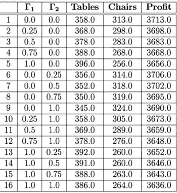
Table 2.2 shows the results of the optimization for various uncertainty budgets. All linear programs and robust formulations in this thesis were solved using Gurobi [7]. Note that when I1 and 1'2 are both 0, the solution is the same as the deterministic case, with a profit of

$3713. However, as the total uncertainty increases, the profit decreases.

the same as the deterministic case. In tests 2 through 5, uncertainty is only present in the carpentry labor hours for chairs and profit is lost. The profit loss is less pronounced when uncertainty is only present in the painting constraint, as in tests 6-9. Because the maximum potential deviation in painting is much smaller, the amount of profit lost is less. Tests 10-15 shows the result when both carpentry and painting are subjected to uncertainty. Note that the uncertainty budget need not be an integer. Finally, the last test is the worst case scenario, with maximum uncertainty budgets for both carpentry and painting constraints.

__ I r2 I Tables Chairs Profit

1 0.0 0.0 358.0 313.0 3713.0 2 0.25 0.0 368.0 298.0 3698.0 3 0.5 0.0 378.0 283.0 3683.0 4 0.75 0.0 388.0 268.0 3668.0 5 1.0 0.0 396.0 256.0 3656.0 6 0.0 0.25 356.0 314.0 3706.0 7 0.0 0.5 352.0 318.0 3702.0 8 0.0 0.75 350.0 319.0 3695.0 9 0.0 1.0 345.0 324.0 3690.0 10 0.25 1.0 358.0 305.0 3673.0 11 0.5 1.0 369.0 289.0 3659.0 12 0.75 1.0 378.0 276.0 3648.0 13 1.0 0.25 392.0 260.0 3652.0 14 1.0 0.5 391.0 260.0 3646.0 15 1.0 0.75 388.0 263.0 3643.0 16 1.0 1.0 386.0 264.0 3636.0

Table 2.2: Chair Coefficient Uncertainty

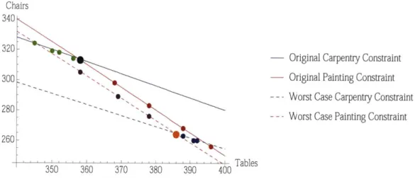
Figure 2-1 includes the worst case constraints and shows change in solution for changing uncertainty budgets.

Chairs 340

320O

Original Carpentiy Constraint

300--- Original Painting Constraint

- - Worst Case Carpentry Constraint

280-- Worst Case Painting Constraint 260

350 360 370 380 390 400

Figure 2-1: Movement of Optimal Solution

The red points show the change in the solution when r2 is held at 0 and F, is varied from 0 to 1. The green points show the change in the solution when 172 is varied from 0 to 1 while F, is held at 0. The purple points show the change when I1 is varied from 0 to 1 while

1F2 = 1. Finally, the blue points show the change when I1 is held at 1 and F2 is varied from

0 to 1. The black point is the deterministic solution, while the orange point is the worst

case solution. Note that not all of the points are located on the constraint. This is because the numbers of tables and chairs made must be integers. Thus, some of the solutions fall

slightly below the constraints. Additionally, notice that the slope of the constraints changes slightly from best to worst case. Because the deviation in the coefficients is small in this problem, the change in slope is difficult to see. It makes sense, however, that when the chair

coefficient is changes, the slope of the constraint changes as well.

Robustness to Uncertainty in Constraint Matrix

The purpose of robust optimization is to provide a solution that will remain feasible despite changes in the parameters of the problem. Comparing the best and worst case solutions in

Table 2.2, we can see that this goal is accomplished. The nominal values of the coefficients

values of I and F2, which are both equal to 1, these coefficients can vary up to 5.5 and 2.05. The solution to the nominal problem is to create 358 tables and 313 chairs, for a total profit of $3713. In this case, the constraints are as follows:

4(358) + 5(313) = 2997 < 3000

3(358) + 2(313) = 1700 < 1700

The painting constraint is binding, but there is a small amount of room for deviation in the carpentry constraint. It is impossible to create any more tables or chairs without violating these constraints. If, however, the true values of the chair coefficients are 5.5 and 2.05, the constraints look like this:

4(358) + 5.5(313) = 3153.5 3000

3(358) + 2.05(313) = 1715.65 1700

The constraints are violated, so the nominal solution is infeasible when the coefficients vary by their maximum allowed deviations. In fact, in order to be able to produce as many chairs and tables as in the nominal solution, an additional 153.5 hours of carpentry labor and 15.65 hours of painting labor would be required. Only then could the manufacturer make the same profit as in the nominal case.

What happens to the feasibility if the F values are less than the worst case? Clearly, F2 cannot be greater than zero. Because the painting constraint is the binding constraint in the nominal case, any change in the painting coefficient for chairs will render the nominal solution infeasible. We do have some room for variation in the carpentry constraint. In fact, as long as IF < 0.019, meaning the carpentry coefficient of the chairs remains below 5.00956, this constraint will not be violated. When F, just exceeds 0.019, the new best solution is

360 tables and 310 chairs, which results in a loss in profit of $3.

When both F values are 1, the robust optimization program solves for a solution that will remain feasible even in the worst case variation, meaning the chair coefficients for car-pentry and painting are 5.5 and 2.05, respectively. At these values, the nominal solution is infeasible. It is also infeasible for any value of the painting coefficient between 2 and 2.05. The nominal solution also becomes infeasible over a large percentage of the range between 5 and 5.5 for the carpentry coefficient. The manufacturer, in choosing the F values, indicated his belief that the true coefficients will be somewhere in the ranges [4.5, 5.5] and [1.95, 2.05]. Of course, any solution to the nominal problem would also be a solution to a problem where these coefficients are actually smaller than the nominal. If it truly takes less time to make and paint a chair, then we can make at least as many chairs as we thought we could before. The infeasibility issues arise when the actual time to make and paint a chair is increased from the nominal. There is only one solution that remains feasible across this whole range, and it is very unlikely that the nominal solution will be feasible. Thus, the robust optimiza-tion soluoptimiza-tion is the safest. However, an addioptimiza-tional analysis measuring the trade-off of profit gained versus the price of paying laborers for extra hours could influence the manufacturer's decision. As state above, an additional 153.3 hours of carpentry labor and 15.65 hours of painting labor would be required to manufacture the nominal solution at the worst case values. If the cost of wages for these hours were less than the profit difference of $377, then of course the manufacturer should just pay for the extra hours. Additional constraints could be added to the linear program to better plan for situations like this.

Unless both constraints are binding in the nominal solution, there will always be some small amount of room for variation where the robust solution is the same as the nominal solution. This is because we are dealing with integer variables. However, in real life appli-cations, it is unlikely that the allowable variation of a coefficient or the F of a row will be so small that the nominal solution remains optimal.

2.3.3

Uncertainty in the Objective Function

The above example demonstrates cardinality constrained optimization for uncertainty in the A matrix. However, this framework is also useful for uncertainty in other parts of the problem. Returning to the furniture example, perhaps the uncertain value is the price that can be charged for each item. This creates uncertainty in the objective function. To deal with this, the objective function can be brought down into the constraint matrix and then treated the same way as the other constraints. In the furniture example, that would look like this: max z subject to 6t + 5c - ( 1q1 + rt + r1) > z 4t + 5c < 3000 3t + 2c < 1700 qi + ric > lYc qi + rit > 2yt t, C, q1, ric, rit > 0 -Yc < c < Yc -Yt < t < Yt

The value F1 represents the uncertainty budget in the new profit constraint. Table 2.3 shows the effect of varying F1.

The first test shows that the results are the same as the nominal case when the uncertainty budget for the first constraint is set to zero. The remaining tests show the result of increasing the uncertainty budget in the first constraint. Notice that the number of chairs and tables changes slightly. This is because the slope of the objective function is changing, so the best point within the feasible region changes. However, the change in the objective function is not enough to force the solution to be located near a different vertex of the feasible region. The last test is the worst case scenario for this problem, with the maximum uncertainty

budget for the profit constraint.

Ir

1 0.0 358.0 313.0 3713.0 2 0.2 358.0 313.0 3569.8 3 0.4 358.0 313.0 3426.6 4 0.6 355.0 316.0 3284.0 5 0.8 355.0 316.0 3142.0 6 1.0 355.0 316.0 3000.0 7 1.2 355.0 316.0 2936.8 8 1.4 355.0 316.0 2873.6 9 1.6 355.0 316.0 2810.4 10 1.8 355.0 316.0 2747.2 11 2.0 357.0 314.0 2684.0

Table 2.3: Objective Function Uncertainty

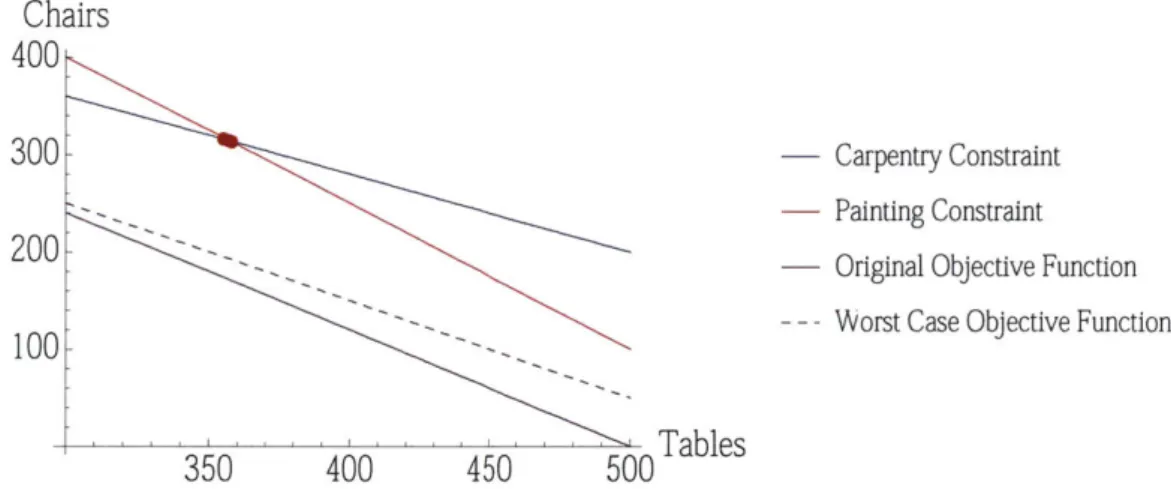
Figure 2-2 shows the change in the objective function as the coefficients are allowed to vary. Notice that the change in the objective function is not enough to change the vertex near which the optimal integer solution is located.

Chairs

400

300.3001 - Carpentry Constraint

-Carpentry Constraint

- Painting Constraint - Original Objective Function -- - Worst Case Objective Function

350 400 450 500 Tables

Figure 2-2: Variation of Objective Function 20C

Robustness to Uncertainty in the Objective Function

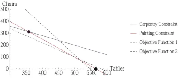
Because the the variables in this problem must be integers, there is some small change in the optimal solution over the range of uncertainty in Table 2.3. Slight changes in the slope of the objective function have the effect of shifting the optimal solution from one integer point near the vertex to another. The value of these solutions decreases as the uncertainty budget increases. The purpose of using robust optimization on the objective value is to provide an estimate of the worst case profit. However, it is possible for variation in the objective function to effect a major change in the optimal solution, not just the objective function value. Figure 2-3 shows the change in the optimal solution with the change in the uncertainty budget.

Chairs

3007

Figure 2-3: Varying Objective Functions

The optimal solution to a linear program occurs at the point where no part of the ob-jective function line is inside of the feasible region. When the variables in the problem are continuous, this means the optimal solution will always occur either at a vertex or along a constraint. In the integer case, the optimal solution will be an integer point close to a vertex. In the nominal case for this problem, the optimal integer solution occurs near the vertex where the two constraints intersect. The purple dashed line represents the nominal objective function and the purple dot is the optimal solution for this objective function. If,

however, the objective function were 3t + c, the solution would occur near a different vertex-the intersection of vertex-the painting constraint and c = 0. This is shown by the black dashed line and black point.

For this objective function, the optimal solution is achieved when 566 tables and 0 chairs are produced, for a profit of $1699. For comparison, the nominal solution of 358 tables and 313 chairs would result in a profit of $1387. In fact, the optimal solution changes when the slope of the objective function exceeds the slope of the painting constraint. So if these two slopes were close to begin with, a small uncertainty budget could effect large changes in the optimal solution. If these slopes are very disparate, then changes in the objective function will only result in changes in the total profit, not the number of tables and chairs that should be made.

2.3.4 Uncertainty in Constraint Limits

If instead, the uncertainty is only in the b vector, the dual of the problem becomes more useful. In the dual, the b vector becomes a row in the dual A matrix, which is easily dealt with using this formulation. Another option that does not require the dual is to subtract the b vector to the left side of the constraint. Create another variable and set it equal to 1. Then treat the b vector as the coefficient of this variable for each row. Now the original robust optimization formulation can be applied to the new constraint matrix. This method is shown below.

max 6t

+

subject to 4t + 5c - 3000x + (F1qI + rix) < 0

3t + 2c - 1700x +(F 2q2 + r2x) < 0 q1 + rix > 1 0 0_YX q2 + r2x > 50yx x -Yx < X < Yx t, C, q1, q2, rix, r2x > 0

The results of varying the uncertainty budget are shown in Table 2.4. Again, the first test shows that the problem is equivalent to the deterministic case when the uncertainty budget is zero. The remaining tests show the effects of varying the uncertainty budgets. Test 10 is the worst case scenario for this formulation.

F1 I2I Tables Chairs Profit

1 0.0 0.0 358.0 313.0 3713.0 2 0.5 0.0 372.0 292.0 3692.0 3 1.0 0.0 386.0 271.0 3671.0 4 0.0 0.5 341.0 326.0 3676.0 5 0.0 1.0 322.0 342.0 3642.0 6 1.0 1.0 350.0 300.0 3600.0

Table 2.4: Constraint Limit Uncertainty

Robustness to Uncertainty in Constraint Limits

Figure 2-4 shows how the constraints move with variations in the b vector. From this figure, it is obvious that the nominal solution, at the intersection of the two solid lines, will be outside of the feasible region when the b vector changes. The optimal solution for the worst case values, on the other hand, is clearly within the feasible region for any values of the b vector up to and including the worst case. Because the solutions for the furniture problem is limited

to integers, there may be some small region around the nominal b vector values in which the nominal solution remains optimal. However, it is so small as to be inconsequential.

In contrast to Figure 2-1, the slope of the lines remains constant in Figure 2-4. The constraints merely shift down, but remain parallel.

Chairs -0Carpentry Constraint 300- -Painting Constraint 280 Tables 340 350 360 370 380

Figure 2-4: Original and Worst Case Constraints

2.3.5 Combined Uncertainty

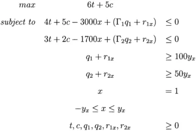
Of course, any combination of these uncertainties-A matrix, objective function, or b vector-is possible. By moving the objective function down into the constraint matrix and moving the constraint limits into the constraint matrix, we can address uncertainty in all three locations-objective function, constraint matrix, and constraint limits-simultaneously. We require three ' values because uncertainty is present in three rows of the problem. A total of eight parameters can be allowed to vary, so we have eight r variables. The resulting formulation is shown here:

max z

subject to 6t + 5c - (P1qi + Tit + nic) > z

4t + 5c - 3000x + (F2q2 + 2t + 2c + 72x) 5 0 3t + 2c - 1700x + (F3q3 + t r3+ c r3+ TU) 0 qi + ?,it > 2t q1 + rc >1c q2 + r2x > 10Ox q2 + r2t > .5x q2 + r2c > .5x q3 + r3x > 50x q3 + r3t > .5x q3 + r3c > .05x t, C, i, ,it, T2x, r2c, 72t, 3x, r3c, r3 > 0

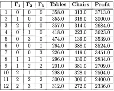
The results of this formulation are shown in Table 2.5. The first test again shows that

this formulation is equivalent to the nominal formulation when the uncertainty budget is zero for every row. Tests 2 and 3 correspond to allowing uncertainty only in the objective function. These values can be verified with the data in Table 2.3.

I1 L' 2 r3 Tables Chairs Profit 1 0 0 0 358.0 313.0 3713.0 2 1 0 0 355.0 316.0 3000.0 3 2 0 0 357.0 314.0 2684.0 4 0 1 0 418.0 223.0 3623.0 5 0 3 0 474.0 139.0 3539.0 6 0 0 1 264.0 388.0 3524.0 7 0 0 3 226.0 419.0 3451.0 8 1 1 1 296.0 330.0 2834.0 9 1 2 2 201.0 381.0 2709.0 10 2 1 1 298.0 328.0 2504.0 11 2 2 2 300.0 300.0 2400.0 12 2 3 3 312.0 272.0 2336.0 Table 2.5: Multiple Uncertainties

The result of the next test does not appear in any of the other tables in this section. With IF, = 0, 1F2 = 1, and 13 = _{0, we are saying that for the coefficients in the second constraint-4,}

5, and 3000-the variation as a percentage of total allowable variation must not exceed 1. This means the sum of the percent variation of the table carpentry coefficient, the percent variation of the chair carpentry coefficient, and the percent variation of the carpentry labor hours available must not exceed 1. For example, the table coefficient may vary by 0.3 of its maximum deviation, the chair coefficient by 0.5, and the labor hours by 0.2. For another example, the labor hour coefficient could be allowed to vary by its maximum deviation, while the table and chair constraints are held at their nominal values. This, too, would result in a total variation of 1. In section 2.3.2, we discussed the results when only the chair coefficient is allowed to vary. If the full uncertainty budget were allocated to the chair coefficient, we would get the same result as test 5 of Table 2.2. if the uncertainty budget were applied to only the labor hours, we would get the same result as test 5 of Table 2.4. The RO calculates which allocation of deviation results in the worst case profit. In this particular case, the worst case is to allocate the entire uncertainty budget to the table constraint, allowing it to

deviate by its maximum deviation, 0.5. This result in a solution of 418 tables and 223 chairs, for a profit of $3623, which is indeed worse than the profits of $3656 and $3671 obtained from allocating the full uncertainty budget to either the chair coefficient or the labor hours, respectively.

In test 5, the uncertainty budget is now 3. Since no single coefficient may deviate beyond

100% of its maximum deviation, the total uncertainty budget must be divided evenly among

the three coefficients. Each of the three coefficients deviates by its maximum amount in this case, for a total profit of $3539.

Test 6 is similar to test 4. The worst case allocation of the uncertainty budget for row

3 allows the table coefficient to vary by its maximum value while holding the other two

coefficients at their nominal values. Test 7 is similar to test 5, with each coefficient of the third constraint being allowed to vary by its maximum deviation.

The remaining tests show the results of various uncertainty budgets for each row. The worst case, in which all eight coefficients are allowed to vary by their maximum deviations, is shown in test 12.

2.4

Summary

Robust optimization is a valuable framework for dealing with real-life problems, which rarely meet the precision required for standard linear programming approaches. Several different approaches have been made, but cardinality-constrained robust optimization is unique in its linearity and level of optimality. The examples in this chapter illustrated the details of the method, including what happens when uncertainty is present in different places in the formulation. The robustness of these results was demonstrated by applying the nominal solution to the altered problem. In some cases, the nominal solution is infeasible when the parameters change. In others, the nominal solution is simply inferior to the robust solution.

Chapter 3

Partially Observable Markov Decision

Processes

This chapter introduces Markov decision processes (MDPs) and three different solution meth-ods for them. The three methmeth-ods are value iteration, policy iteration, and linear program-ming. Then, it discusses partially observable Markov decision processes (POMDPs) and the difficulties associated with solving them. Two solution methods are provided. Multiple examples are used to illustrate these problems and their solution methods. All MDP and POMDP solutions in this thesis were calculated using APPL [14].

3.1

Markov Decision Processes

Markov decision processes (MDPs) are used to model sequential decision making. An agent with a specific goal has a set of available actions. An MDP determines the optimal policy, which specifies which action the agent should take based on the current state of the system. A Markov decision process is defined by a set of four components:

S Set of possible states

A Set of possible actions

R Reward function

T State transition matrix for each action

A state of a system is its current condition.The set of possible states, S, encompasses both the state of the agent and the state of its environment. The state is fully observable, meaning at any time the current state of the system is known.

The set of possible actions, A, lists the actions available to the agent. Actions can be repeated and not every action must be used.

The reward function maps actions and states to rewards or costs. Some actions may have costs or rewards that are constant across different states. Some actions may be more valuable in certain states than in others.

The transition matrix T describes how the state of the system changes when an action is taken. The transition probabilities are independent of the state history, meaning that the effects of a specific action depend only on the current state, not on the path taken to arrive at the current state. This is known as the Markov property.

3.2

MDP Example

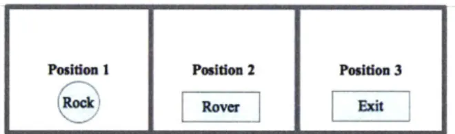
Consider this very simple MDP. A rover on the surface of Mars is constrained to move in a 1x3 matrix, labeled from left to right as positions 1, 2, and 3, respectively. The purpose of this rover is to gather rock samples and then reach an exit state. The exit state is position 3. The rover is only supposed to collect good rock samples. If the rock is bad, the rover should leave it and move directly to the exit. The rock is in position 1. There are two components of the state for this example: position of the rover and the quality of the rock sample. The rover starts in position 2 and the rock is of good quality, as shown in Figure 3-1.

Posiion 1 Posiden 2 Posidon 3

EIZ

i]

Ei']

Figure 3-1: Rock Sample Problem Environment

The actions available to the rover are Move Left, Move Right, and Collect. The reward function specifies a reward or cost of taking each action in any given state. The transition probability matrix encodes how each action changes the state of the system. Note that each combination of rover location and rock quality is a state. Thus, there are six states, shown in Table 3.1 and Figure 3-2

Sta 1 2 3 4 5 6 te Rover Position Ro 1 1 2 2 3 3

Table 3.1: Rock Sample

ck Quality Good Bad Good Bad Good Bad States

Figure 3-2: Rock Sample States

State I State 3 State 5

Position 1 Position 2 Psto Good Rock GodRock G oodtiRock

State 2 State 4 State 6

Position I Position 2 Position 3

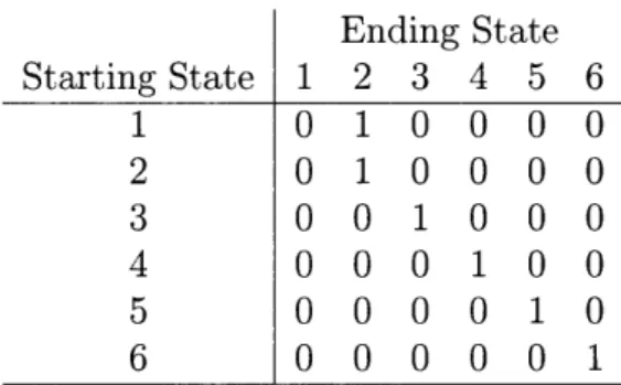
The transition matrices are shown in Tables 3.2 to 3.4. The transitions are deterministic, which makes this a very simple problem that could easily be solved by hand. Often, MDP transitions are probabilistic. In this case, though, probabilistic transitions would not make much sense. When a rover is given a direction to travel, there is no reason why it would move in the opposite direction. Probabilistic transitions could be useful for the Collect action, because it may be possible for the rover to fail to grab the rock. In this example, however, we will assume that the rover is very accurate and does not miss the rock.

Starting State 1 2 3 4 5 6 Table 3.2: Move Starting Stat 1 2 3 4 5 6 Table 3.3: Move 1 1 0 1 0 0 0 Left Ending State 2 3 4 5 0 0 0 1 0 0 0 0 0 1 0 0 0 0 0 0 0 0 Transition 6 0 0 0 0 0 0 0 0 1 0 0 1 Matrix Ending State 1 2 3 4 5 6 0 0 1 0 0 0 0 0 0 1 0 0 0 0 0 0 1 0 0 0 0 0 0 1 0 0 0 0 1 0 0 0 0 0 0 1 Right Transition Matrix

Ending State Starting State 1 2 3 4 5 6 1 0 1 0 0 0 0 2 0 1 0 0 0 0 3 0 0 1 0 0 0 4 0 0 0 1 0 0 5 0 0 0 0 1 0 6 0 0 0 0 0 1

Table 3.4: Collect Transition Matrix

For every action in every state, there is an associated reward. Tables 3.5 through 3.7 contain these rewards.

State 1 2 3 4 5 6 Reward -5 -5 -5 -5 -50 -50

Table 3.5: Move Right Rewards

State 1 2 3 4 5 6 Reward -50 -50 -5 -5 0 0

State Reward 1 75 2 -500 3 -50 4 -50 5 -50 6 -50

Table 3.7: Collect Rewards

The state transition matrix for the actions Move Left and Move Right do not depend on the quality of the rock, nor do they affect the quality of the rock. Thus, if the rover is in state 3 and moves left, it moves to state 1. If it is in state 3 and moves right, it moves to state 5. The rock quality remains unchanged. The reward matrix for Move Right and Move Left include penalties for attempting to move beyond the confines of the 1x3 world. The action Collect does not affect the current position of the rover, but it can affect the current state. If the rover is in state 1 and Collects the good rock, the rock quality changes to Bad and the rover moves to state 2. This is done so that the rover cannot continually recollect a good rock. The rock can only be collected once. If the rover is in state 2 and attempts to Collect the bad rock, a large penalty is incurred. If the rover is in position 2-hence, states 3 or 4-and chooses to Collect, a penalty is incurred because there is no rock there to sample. Notice that position 3 is an absorbing state. Once position 3-states 5 and 6- has been entered, no action will move the rover away. The zero cost of moving left from either state 5 or 6 make these states desirable end states. All of the transitions are deterministic, which makes this

a very simple MDP with an obvious solution.

In this case the rover starts in position 2 and a rock of good quality is located in position 1. By observation, it is clear that the best plan is for the rover to Move Left, Collect, Move Right, Move Right, then always Move Left. This will allow the rover to collect the good sample, travel to the exit position and accrue no more cost. Table 3.8 shows how each action changes the state of the system.