Distributionally robust optimization for design under partially observable uncertainty

Distributionally Robust Optimization for Design

under Partially Observable Uncertainty

by

Michael George Kapteyn

BE. (Hons) Engineering Science, The University of Auckland (2016)

Submitted to the Department of Aeronautics and Astronautics

in partial fulfillment of the requirements for the degree of

Master of Science in Aeronautics and Astronautics

at the

MASSACHUSETTS INSTITUTE OF TECHNOLOGY

June 2018

Massachusetts Institute of Technology 2018. All rights reserved.

Signature redacted

A uthor ...

Department of Aena ics and Astronautics

May 24, 2018

Signature redacted

Certified by...K

V//

Karen E. Willcox

Professor of Aeronautics and Astronautics

Thesis Supervisor

Accepted by

...

Signature redacted

Hamsa Balakrishnan1

Associate Professor of Aeronautics and Astronautics

Chair, Graduate Program Committee

MASSACHUSETTS INSTITUTE

OF TECHNOLOGY

JUN 28 2018

LIBRARIES

Distributionally Robust Optimization for Design

under Partially Observable Uncertainty

by

Michael George Kapteyn

Submitted to the Department of Aeronautics and Astronautics on May 24, 2018, in partial fulfillment of the

requirements for the degree of

Master of Science in Aeronautics and Astronautics

Abstract

Deciding how to represent and manage uncertainty is a vital part of designing complex systems. Widely used is a probabilistic approach: assigning a probability distribution to each uncertain parameter. However, this presents the designer with the task of assuming these probability distributions or estimating them from data, tasks which are inevitably prone to error. This thesis addresses this challenge by formulating a distributionally robust design optimization problem, and presents computationally efficient algorithms for solving the problem. In distributionally robust optimization (DRO) methods, the designer acknowledges that they are unable to exactly specify a probability distribution for the uncertain parameters, and instead specifies a so-called ambiguity set of possible distributions. This work uses an acoustic horn design problem to explore how the error incurred in estimating a probability distribution from limited data affects the realized performance of designs found using traditional approaches to optimization under uncertainty, such as multi-objective optimization. It is found that placing some importance on a risk reduction objective results in designs that are more robust to these errors, and thus have a better mean performance realized under the true distribution than if the designer were to focus all efforts on optimizing for mean performance alone. In contrast, the DRO approach is able to uncover designs that are not attainable using the multi-objective approach when given the same data. These DRO designs in some cases significantly outperform those designs found using the multi-objective approach.

Thesis Supervisor: Karen E. Willcox

Acknowledgments

Firstly I would like to thank Professor Karen Willcox, who provided me with an incredible opportunity when she welcomed me into her research group, and who con-tinues to offer me unrivaled guidance, teaching, mentorship, and support. I would also like to thank Professor Andy Philpott for the initial idea for this research, and for his

guidance and insightful, thought-provoking discussions throughout it's completion.

I would like to thank the SUTD-MIT International Design Center for providing

me with the opportunity to visit Singapore, and Karen, Max and Alex for making the experience an enjoyable and memorable one.

I would also like to thank all of my fellow students in the Aerospace Computational Design Lab (ACDL) for their support, friendship, and welcome distractions from productive work. Additional thanks go out to my housemates Conor, Tim, Andrew and Gary, as well as Richard, Ben, Jeff, Nicole and the rest of my expatriated Kiwi friends for providing me with a home away from home.

Last but certainly not least I would like to thank my family. Mum, Dad, Carmen, Andy, and Megan-Thank you for your everlasting love and support. I hope I can make all of you proud.

None of this would have been possible without financial support. This work was supported in part by AFOSR grant FA9550-16-1-0108 under the Dynamic Data Driven Application Systems Program, by the Defense Advanced Research Projects Agency [EQUiPS program, award W911NF-15-2-0121, Program Manager F. Fahroo],

by a New Zealand Marsden Fund grant under contract UOA1520, and by the

TABLE OF CONTENTS

Nomenclature 9 List of Abbreviations 13 List of Figures 15 List of Tables 17 1 Introduction 19

2 Design Optimization Under Partially Observable Uncertainty 23

2.1 Direct optimization using sample average approximation . . . . 23

2.2 Motivating example: the challenges of optimization under uncertainty 26

2.2.1 Model problem formulation . . . . 26

2.2.2 The consequences of partial observability . . . . 32 2.3 Robustness through multi-objective optimization . . . . 35

3 Distributionally Robust Design Optimization 43

3.1 Form ulation . . . . 43 3.2 Constructing the ambiguity set and finding the worst-case distribution 46

3.2.1 L2-norm ambiguity . . . . 47 3.2.2 Kullback-Leibler (K-L) divergence ambiguity . . . . 52

4 Performance of the Distributionally Robust Approach 57

4.1 M ean-risk tradeoff . . . . 57

4.2 Sizing the ambiguity set . . . . 61 4.3 Effect of the underlying distribution . . . . 68

5 Conclusions and Future Work 73

Appendix A Additional Results for the L2-Norm Ambiguity Set 75

NOMENCLATURE

Greek Symbols

Symbol Description

Fin Computational boundary at the acoustic horn inlet FN Computational Boundary at the acoustic horn walls

IFR Truncated absorbing boundary of the computational domain in the acoustic horn problem

K Kolmogorov-Smirnov (K-S) distance between a random sample and the true underlying distribution

A Mean versus standard deviation trade-off parameter in the Multi-Objective Optimization M

Average of the argument over T samples

Q"M _{Space of all vectors of representing discrete probability measures}

over m support values

0() CVaR10 of the argument over T samples

Roman Symbols

Symbol Description

a Half-width of the horn inlet

b Half-width of the horn outlet

'D Distributionally robust design optimization problem

DL2(-,-) Function measuring the K-L divergence between two discrete prob-ability vectors

DKL ( Function measuring the L2-norm of the difference between two

dis-crete probability vectors

e. Unit vector with a 1 in position j

i Imaginary unit, I

k Wave-number in the acoustic horn problem

L Length of the horn from inlet to outlet M Multi-objective design optimization problem

m Sample size

'P Full observability design optimization problem

P Ambiguity Set

p Empirical distribution from a sample of the uncertain parameters

PQ Probability density function of the quantity of interest

p* Worst-case distribution within the ambiguity set

Pu Probability density function of the uncertain parameters

Q

Quantity of interest (Qol)

R Radius of the truncated absorbing boundary in the horn model

r Radius of ambiguity

Normalized radius of ambiguity (0-1)

S Sample average approximation-based design optimization problem

s Reflection coefficient of the acoustic horn

Sm Standard deviation in performance of design xm under the true

distribution Pu

T Number of random samples used in computational experiments

u Vector of uncertain parameters

U Space of possible uncertain parameter vectors

v Non-dimensionalized pressure

x Vector of design variables

X Space of possible design vectors

xec True optimal design-an optimizer of '

xmI Optimal design computed using a sample size m

z Dummy variable used in the optimization over a K-L divergence ambiguity set

zoo True optimal mean performance-the optimal objective value in 'P

Zm Mean performance of design xm under the true distribution P,

LIST OF ABBREVIATIONS

CDF cumulative distribution function. 61 CVaR conditional value-at-risk. 32, 38

DRO distributionally robust optimization. 3, 16, 21, 43-48, 52, 57-60, 65-71, 74-80 K-L Kullback-Leibler. 7, 11, 16, 21, 52-54, 58-60, 62, 65-68, 70, 71, 73-76

K-S Kolmogorov-Smirnov. 9, 16, 61, 62, 65-67, 69, 71, 75, 77-79

MOO multi-objective optimization. 15, 16, 21-23, 35, 37-39, 42, 45, 48, 58-60, 73 QoI quantity of interest. 15, 19, 24, 28-30, 33, 58, 75

SAA sample average approximation. 17, 21-26, 32, 35, 40, 44, 46, 59-61, 63, 69, 73, 76

14

2:Eti?'P."

A'

t-V

7''

WP'''f3at"--"??

.7

ny~~y

-t-I+'l-.wir-p?.Ytd~f'PurjfJM

-.

eg

n

are

..

piw

rrgg

-ao--fj .1

stur~prEloa

t

: !

ot-

s-r/fz-

s

tar

y:-9:w-ppe-yr-.

..... ...;'-' -.7 .-..'..''. ' ....

LIST OF FIGURES

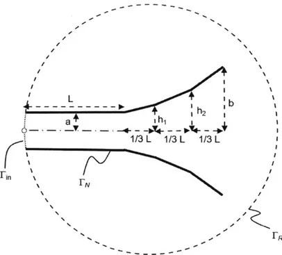
2-1 The geometry of the acoustic horn model (Adapted from Ng et al.1). The design variables used in this thesis are h, and h2, while the

re-maining parameters shown are considered fixed. . . . . 27

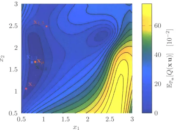
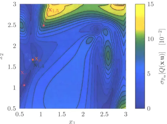
2-2 Mean value of the quantity of interest (Qol) over the acoustic horn design space, for a uniformly distributed wave number. . . . . 29 2-3 Standard deviation in the QoI over the acoustic horn design space, for

a uniformly distributed wave number. . . . . 30

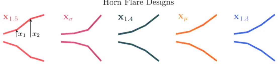
2-4 _{Performance of designs that exhibit optimal mean performance (x,),} minimal variation in performance (x,), or optimal performance at a particular value of the uncertain variable (x1.3, x1.4, x1.5). . . . . 31 2-5 Histograms showing the mean performance of designs computed from

T = 500 sample draws of size m. The optimal, mean, and CVaRio

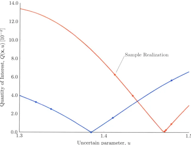
values over all sample draws are indicated. . . . . 33 2-6 Performance of two designs over the uncertainty space U. These are

the designs that exhibit the best and worst mean performance over all designs computed using different sample draws of m = 5 realizations of the random variables. . . . . 34

2-7 Mean versus standard deviation curves generated using multi-objective optimization (MOO), with varying sample size, for the acoustic horn design problem. Each curve corresponds to a sample size m = 5, 10, 20, and is computed by averaging over T = 1000, 600, 200 samples,

respec-tively. Each point on a curve corresponds to a particular value of

A E [0, 1]... 38

2-8 Mean versus CVaRio curves generated using MOO, with varying sam-ple size, for the acoustic horn design problem. Each curve corresponds to a sample size m = 5,10, 20, and is computed by averaging over

T = 1000, 600, 200 samples, respectively. Each point on a curve

corre-sponds to a particular value of A E [0, 11. . . . . 39 2-9 Performance over the uncertainty space, U, of designs computed by

solving M(A), with A = 0, 0.5, 0.95 and the worst-case sample of size

m = 5 realizations. . . . . 40 2-10 Performance over the uncertainty space U of designs computed using

A = 0, 0.5, 0.95 and the best-case sample of size m = 5 realizations of

the uncertain parameter. . . . . 41

3-2 Plot of K-L ambiguity sets in 3-dimensional barycentric co-ordinates. 4-1 Mean-Risk tradeoff curves for designs computed using sample draws

of size m = 5, 10,20 and the DRO approach with L2-norm and K-L

divergence ambiguity sets. Also shown are the corresponding curves for the MOO approach, as well as the true optimal performance. . . . 59

4-2 Surface plot showing the relationship between the K-S statistic of a sample, the ambiguity set size, and the resulting design performance using uniformly distributed samples of size m = 5 and the DRO

ap-proach with a K-L divergence ambiguity set. . . . . 65

4-3 Surface plot showing the relationship between the K-S statistic of a sample, the ambiguity set size, and the resulting design performance using uniformly distributed samples of size m = 10 and the DRO

approach with a K-L divergence ambiguity set . . . . . 66

4-4 Surface plot showing the relationship between the K-S statistic of a sample, the ambiguity set size, and the resulting design performance using uniformly distributed samples of size m = 20 and the DRO approach with a K-L divergence ambiguity set. . . . . 67

4-5 Comparison between the uniform and normal probability density func-tions used in the acoustic horn design experiments. . . . . 68

4-6 Comparison between mean-risk trade-off curves for designs computed using normally distributed and uniformly distributed uncertainty. Re-sults are for sample sizes m = 5,10, 20 and the DRO approach with

K-L divergence ambiguity set. . . . . 70

4-7 Surface plot showing the relationship between the K-S statistic of a sample, the ambiguity set size, and the resulting design performance using normally distributed samples of size m = 10 and the DRO ap-proach with a K-L divergence ambiguity set. . . . . 71 A-1 Surface plot showing the relationship between the K-S statistic of a

sample, the ambiguity set size, and the resulting design performance using uniformly distributed samples of size m = 5 and the DRO ap-proach with a L2-norm ambiguity set. . . . . 77 A-2 Surface plot showing the relationship between the K-S statistic of a

sample, the ambiguity set size, and the resulting design performance using uniformly distributed samples of size m = 10 and the DRO

approach with a L2-norm ambiguity set. . . . . 78 A-3 Surface plot showing the relationship between the K-S statistic of a

sample, the ambiguity set size, and the resulting design performance using uniformly distributed samples of size m = 20 and the DRO approach with a L2-norm ambiguity set. . . . . 79

A-4 Comparison between mean-risk trade-off curves for designs computed using normally distributed and uniformly distributed uncertainty. Re-sults are for sample sizes m = 5,10, 20 and the DRO approach with

L2-norm ambiguity sets. . . . . 80 16

LIST OF TABLES

4-1 Best average mean and average CVaRio values attained by each method for sample sizes of m = 5, 10, 20. Also shown is the percentage

reduc-tion in the optimality gap relative to the sample average approximareduc-tion

CHAPTER 1

INTRODUCTION

In designing a system to achieve optimal performance, the designer typically evalu-ates system performance using some quantity of interest (QoI) (e.g., cost, efficiency, weight). The QoI depends on design variables, which the designer wishes to select optimally. Typical design variables include geometric quantities (e.g., span, sweep angle for an aircraft wing), material properties (e.g., material stiffness, density for an aircraft wing spar), or operational decisions (e.g., nominal altitude for an aircraft). The QoI will also depend on other parameters which are out of the designers control. Furthermore, in any real-world system the designer may have imperfect knowledge of their true values, rendering these parameters uncertain. Typical examples of such uncertain parameters in the design of an aircraft are windspeed (and thus operational Mach number), or cargo weight.

Computational modeling of the system of interest provides the designer a means to cheaply and rapidly explore how changes in the underlying parameters affect the output quantity of interest, and thus supports more informed design decisions. We consider the setting in which the designer has access to a high-fidelity computational model of the system of interest. The model takes, as input, values for the design variables and the uncertain parameters, and returns an accurate evaluation of the QoL. In practice, such computational models are often complex, proprietary, legacy, and/or written in poorly documented code that the designer may not have time to decipher. With these settings in mind, we treat the model as a black-box. This means we assume no knowledge of the model structure or the behavior of the output variable

and its functional relationship to input variables. This makes the design methodology discussed herein general in the sense that it can be applied to any system, provided the designer has a computational model with input and output as described above.

The field of design optimization under uncertainty concerns the specification, rep-resentation, and treatment of uncertain parameters during a design process. The importance of considering the nature of the uncertain parameters in engineering de-sign has long been established," the primary reason being that methods that simply consider all parameters to be deterministic tend to over-fit designs to the chosen pa-rameter values. This often results in degraded performance of the system when it is exposed to the true uncertain operating environment.5'6

One decision a designer must make is in how to characterize and represent the uncertainty. The most prevalent approach is to treat the uncertain parameters as random variables, with each parameter being assigned a probability distribution de-scribing how it varies.2'5 Other treatments and representations of uncertainty have also been established,7 such as interval or set-based uncertainty,8-10 and possibility theory." In this work we focus on the case of probabilistic uncertainties, where the designer must specify a probability distribution for the uncertain parameters.

In practice the designer will never have perfect knowledge of how the underlying system parameters vary, and thus they will not have access to the exact probabil-ity distribution governing an uncertain parameter. Consequently, the designer will be forced to assume a probability distribution, or to estimate it from known data, processes that will always be prone to error.

Fortunately, the designer usually has some incomplete knowledge about the uncer-tainty, which can help mitigate this error. In this case we say the designer has partial

observability over the uncertainty. One situation in which partially observable

un-certainty commonly arises is the case when the designer has no knowledge about the distribution of uncertain parameters itself, but instead has access to a sample of pa-rameter values drawn from this distribution. This is the case, e.g., when the designer takes discrete measurements of the uncertain parameters. In this work we will con-sider this scenario, denoting by m the size of the sample (number of measurements).

Of particular interest is the case where the sample size, m, is low. This represents

the situation where only limited data are available to characterize the probability distribution.

Recently, a body of work has emerged from within the optimization community studying an approach that explicitly accounts for the fact that one is never able to exactly specify a probability distribution in practice.12_-8 _{This approach, called} distributionally robust optimization (DRO), weakens the assumption of specifying a single probability distribution for the uncertain parameters. Instead, it only requires the designer to select a set of possible probability distributions-the optimization considers all distributions within this set.

In this work we explore how imperfect knowledge of uncertainties affects the per-formance of traditional optimization under uncertainty methods. In particular, we show that these methods often produce designs that perform poorly when realized un-der the true distribution of uncertainty. We then present a formulation of the design optimization as a DRO problem. This formulation explicitly seeks designs that are robust to deviations in the distribution of the uncertainty. We present computation-ally efficient algorithms for solving the DRO problem, when the set of distributions is constructed using either the L2-norm or the Kullback-Leibler (K-L) divergence.

We apply this formulation to a model design problem and show that it outperforms traditional design optimization under uncertainty methods when the uncertainty is only partially observable.

The outline of this thesis is as follows. Chapter 2 formulates the problem of de-sign optimization using only m, realizations of the uncertain parameters and presents two traditional methods for solving this problem using sample average approxima-tion (SAA), and multi-objective optimizaapproxima-tion (MOO). A model design problem is also presented, which serves as a motivating example to illustrate the challenges as-sociated with design under partially observable uncertainty. Chapter 3 presents a formulation of the design problem as a DRO problem, and presents algorithms for solving the resulting optimization problems. Chapter 4 presents the results of the DRO approach applied to the model design problem. These results are used to

an-alyze the performance of the approach, and compare it to both the SAA and MOO approaches. Finally, Chapter 5 concludes the thesis and suggests possible areas to explore in future work.

CHAPTER 2

DESIGN OPTIMIZATION UNDER

PARTIALLY OBSERVABLE UNCERTAINTY

In this chapter we formulate a design optimization under uncertainty problem adapted to the setting in which the designer only has access to a sample of realizations of the uncertain parameters. In Section 2.1 we introduce a methodology for optimizing the mean performance of designs using sample average approximation (SAA). In Section 2.2 we introduce a model design problem, to which we apply the SAA approach and illustrate the consequences of partial observability. Finally, Section 2.3 discusses multi-objective optimization (MOO), and explores how this widely used approach to optimization under uncertainty performs in the partial observability setting.

2.1

Direct optimization using sample average

approx-imation

We denote the vector of design variables by x E X, where X is the feasible design space encoding constraints on the design. To represent the uncertain parameters, we define a probability space (Q, Y, Pu) with sample space Q, --algebra F, and probability measure Pu. We define the random variable u : Q - U, which has dimension equal

to the number of uncertain parameters in the design problem. The uncertainty space,

U, represents the space of all possible realizations of the random variable, u. We use subscripts to denote particular realizations of the uncertain parameters, i.e.,

U1

=

u(wo)

for some wi E Q. We represent the QoL of our system as a function,

Q

(x, u),

of the design variables x, and the uncertain variables, given by the random variable u. As the QoI,

Q

(x, u), is a function of the random variable u, it too is a random variable, with probability measure denoted PQ. Thus, the performance of a design x is completely characterized by the distribution PQ. Note that the randomness in the QoI is induced only by the randomness in u. In a slight abuse of notation, we will use Q(x, ui) to denote the deterministic value of the QoI evaluated at a realization of the uncertain parameters, ui. The problem of design optimization under uncertainty is thus to find a set of optimal design variables that produce a favorable distribution of performance, PQ.

In this work we will be focus on optimizing the mean of the distribution in design performance. In this case, assuming that a lower QoI is favorable, the optimization problem we wish to solve is

'P: min Eo [Q (x, u)]. (2.1)

xEX

We denote the optimal objective value of ' by Z,, and a corresponding minimiz-ing design by x,. A key limitation in solvminimiz-ing 'P is that it requires the designer to have exact knowledge of the probability distribution, P, governing the uncertain parameters. In practice the designer will not have complete knowledge of the exact distribution of the uncertainty. In the setting we consider, the designer has access to a sample of m realizations of the uncertain parameters, drawn from the distribution Pu. Consequently, the designer will be forced to use this sample to make an assump-tion about the true probability distribuassump-tion, with unknown impacts on the resulting optimal design.

In this setting, a simple and commonly used approach is to use SAA. This amounts to approximating the true distribution Pu using the empirical distribution p associ-ated with the sample. In this case

j1,..

,pm denote the likelihood that the uncertain parameters u are realized as u, ... , um respectively. This approach is justified by the fact that as m. -+ o the empirical distribution p is will converge to the true

dis-24

- - IM, 11 VM"M. - P , -- -- , , - I IMM T ,1.11,V , ' 11r,", ',,,,,,"In, 'I' l"vn"lprl" ll" ",,",,P l-", ,," ,,Im- , ,IIKI."""M ,11mlrlm"?.","","",,', ',tlif7lr 1.11Mlt",1-1"q"",","T,",,' '' I I 1 -1 1- 1 1 "1.""", -11. . I-, I'll -- .. . ... ....

tribution Pu for most well-behaved distributions encountered in practice. For a given random sample u1,..., um, with associated empirical distribution

p,

we use SAA to write a finite sample analogue to 'P:

5: min E

[Q(x,u)

= mmin EpiQ(x, ui). (2.2)

xEX xEX

We denote the optimal objective value of 8 by Zm, and the corresponding optimal design by xm. Note that

Zm

is the expected performance of xm under the sample

distribution ]. In practice, what we really care about is how the design xm performs

under the true distribution Pu. To this end, we define the expected performance of the design xm under the true distribution of uncertainty, Pu, and denote this by

Zm = Ep [Q (xm, u)] . (2.3)

Note that

Zm

is able to be calculated by the designer, as it requires only the sampled values of the uncertainty, whereas Zm is not observable by the designer, since it requires knowledge of the true distribution P,.

As m -+ oc we expect 'P and 8 to be equivalent, so that Zm -4 Z, and x -+ x,0.

However, for finite m this approximation will be subject to sampling error. Conse-quently, the solution x, obtained by the designer in the finite sample setting will

differ from the true solution x,. Moreover, xm and Zm will vary between different draws of the random sample. If the empirical distribution p generated by a partic-ular sample draw is a good approximation of the true distribution Pu, then we can reasonably expect x,, to be close to the true optimal design x.. On the other hand, if the sample is not representative of the true distribution P, then x, may differ greatly from the true solution x,, and the corresponding design performance, Zm, may be poor.

The designer has no control or a priori knowledge of whether a particular sample draw is representative of the true distribution. We thus seek design methodologies that are robust to this sampling error, in the sense that over all possible sample

draws the methodology consistently results in designs that perform well under the true distribution. To this end, we will be primarily interested in the performance of designs averaged over all possible sample draws of size m. We will also be interested in the risk level of the methodology, as indicated by how designs perform in the worst-case sample draws.

2.2 Motivating example: the challenges of

optimiza-tion under uncertainty

In Section 2.2.1 we introduce a motivating example: the problem of designing an acoustic horn for maximum efficiency subject to an uncertain operating condition. In Section 2.2.2 we apply the SAA approach outlined in Section 2.1 to the horn design problem, and investigate how partial observability affects the performance of the resulting designs.

2.2.1

Model problem formulation

In this section, we introduce an example design problem that will be used throughout this thesis to explore different design methodologies, and illustrate various aspects of their performance. We suppose that we are tasked with optimizing the design of an acoustic horn in order to minimize the amount of internal reflection present, and thus maximize the efficiency of the horn. In order to analyze how the design of the horn affects the amount of internal reflection, we utilize a computational model. A brief summary of the model is presented in Figure 2-1 below and the description that fol-lows. For more details on the theory behind the acoustic horn and the computational model used, we refer the reader to References 19,20 and 21.

+ h, L

1/3 L 1/3 L 1/3 L

rN

Iin I

Figure 2-1: The geometry of the acoustic horn model (Adapted from Ng et aL.').

The design variables used in this thesis are h1 and h2, while the remaining parameters

shown are considered Eixed.

The exterior domain is truncated by a circular absorbing boundary of radius

R = 25. The non-dimensional horn geometry is axisymmetric and is parameterized

by five variables. We consider three of these to be fixed parameters: the horn inlet

length L = 5, and half-width a = 0.5, and the outlet half-width b = 3. The remaining two variables are design variables h, and h2, corresponding to the half-widths at two uniformly spaced points in the horn flare (see Figure 2-1). Both design variables hi, and h2 are constrained to lie within the interval [a, b) =0. 5, 3 ]. The governing

equation is the non-dimensional Helmholtz equation,

V2V + k 2V = 0, (2.4)

where v is the non-dimensionalized pressure, and k is the wave-number, which we treat as the uncertain operating condition of the horn. The boundary conditions on

the horn inlet

Fin,

horn surface FN, and far field boundary FR are given by

Fin ikv + = 2ik, (2.5)

N: On -0, (2.6)

FR: a - (ik - -L + 8R(1 kR) , (2.7)

where n is a unit vector normal to the corresponding boundary, and i =

v

.

The governing equation is solved to compute v using a reduced basis finite element model with n = 116 basis vectors. The QoI for the acoustic horn model is the reflection coefficient:

S

= f

vdf-1

, (2.8)

which is a fractional measure describing how much of an incoming wave is internally reflected in the horn, as opposed to being transmitted out into the environment. It is thus considered a measure of the horn efficiency, with a lower reflection coefficient giving more favorable performance. Thus, framing the acoustic horn design problem using the notation introduced in Section 2.1, we have:

Design variables: x = [h1, h2 ]T, (2.9)

Design space: X = [0.5, 3 ] x [ 0.5, 31, (2.10)

Uncertain parameters: u = k, (2.11)

Uncertainty space: U = [1.3,1.5], (2.12)

Output Qol Q (x, u) = s. (2.13)

We perform an exploratory analysis of the acoustic horn design space to show how the uncertain wave number affects the reflection coefficient for different horn designs. For this study, we suppose that the wave number follows a fixed truth probability distribution

u - P,, = Uniform(1.3, 1.5). (2.14)

The design points explored comprise a 50 x 50 point, uniformly spaced grid in the

de-sign space X. For each dede-sign, the mean and variance of the Qol under the uniformly

distributed uncertainty is computed using 10-point Gaussian quadrature. Figures

2-2 and 2-3 show contour plots of the mean and standard deviation of the reflection

coefficient over the design space X.

3

2.5

60

2

40

1.5

20

0.5

0

0.5

1

1.5

2

2.5

3

x

₁

Figure 2-2: Mean value of the QoI over the acoustic horn design space, for a

uni-formly distributed wave number.

We see that the reflection coefficient has a non-linear dependence on the design

variables. Horn designs in which x,

> X2

result in poor mean performance. This is

expected since such designs feature a concave horn flare, resulting in a high degree

of internal reflection. We denote the design that achieves optimal (minimal) mean

reflection coefficient x,,, and the design that achieves minimal standard deviation

in the reflection coefficient by x,. The fact that these designs are distinct suggests

that it is possible to trade-off between improving the mean performance of the

horn

design, and reducing the degree of variability in this performance. This type of

mean-standard deviation tradeoff will be explored further in Section 2.3.

3

15

2.5

10

0

2

1.5

5

1

0.5

0

0.5

1

1.5

2

2.5

3

X1

Figure 2-3: Standard deviation in the QoI over the acoustic horn design space, for

a uniformly distributed wave number.

In addition to these designs, Figures 2-2 and 2-3 also show three point-wise

opti-mal designs. These are the designs that achieve optiopti-mal performance at point-wise

values of the uncertain parameter, i.e. wave numbers of u = k = 1.3, 1.4, and 1.5,

respectively. Figure 2-4 shows the horn flare geometry of each of the aforementioned

designs, and the corresponding design performance-given by the Qol-over the range

of the uncertain variable.

We see that designs x1

.

3, x1.4 and x1. all exhibit low reflection at the corresponding

design wave numbers, but also exhibit reduced off-design performance. We also see

from the performance of x, that it is possible to obtain a horn design with consistent

performance over the range of wave numbers, however, this comes with the downside

that QoI is relatively high everywhere. In fact, the performance of x, ends up being

superior to x, at almost all wave numbers. In this case we say that x, stochastically

dominates x,, since it performs better at every point in uncertainty space.

Horn Flare Designs

Xy

X2#

L

3

Design Performance over the Uncertainty Space, U

25 20 15 * 10 0x O-4~ 0 1.3 1.4 1.5 Uncertain parameter, u

Figure 2-4: Performance of designs that exhibit optimal mean performance (x,), minimal variation in performance (x,), or optimal performance at a particular value

2.2.2 The consequences of partial observability

In this section we apply the SAA approach to the acoustic horn design problem. We

simulate T sample draws, each consisting of m random realizations from P,. For

each draw t = 1, ... , T, we solve 8 using an interior point methoda to obtain xm. We

then evaluate Zm, the performance of

xm

under the true distribution P,, by solving

Eqn. 2.3 using 10-point Gaussian quadrature.

In order to evaluate how the methodology performs across all sample draws, we

compute the average of Zm over the T sample draws, denoted by

1 T

1-p(Zm) = E [f{Zm,.. Z }] = T

:ZM,

(2.15)

t=1

where Z denotes the value of Zm in sample draw t. We evaluate the risk level of

the methodology using the notion of conditional value-at-risk (CVaR) (sometimes

referred to as expected shortfall (ES) or expected tail loss (ETL)). In our setting, the

CVaR at level 10% (CVaRio) is defined as the expected value of the worst 10% of all

sample draws. We approximate the true CVaRiO using T sample draws. Assuming

we have ordered the sample indices so that Z,

...

, ZT

is in ascending order, we can

define the approximate CVaRiO of Zm, denoted

q(Zm),

as

#(Zm) = E

[{Z

I t > 0.9T}] .

(2.16)

For the sake of comparison, we also compute

x,

and Z,. Recall that these are the

solutions to the full optimization problem ' (Eqn. 2.1), which requires knowledge of

the true distribution P.. This problem is again solved using 10-point quadrature, this

time using the empirical distribution support and probabilities as quadrature nodes

and weights respectively. We simulate T

=

500 realizations of random samples. For

each random sample we compute an optimized design, and evaluate the mean design

performance under the true distribution Zm, as described above. Figure 2-5 gives a

histogram of Zm values across the 500 sample draws, for sample sizes m = 5, 10, 20.

aAs implemented in the function fmincon, included in the MATLAB Optimization Toolbox2 2

m =5

8

6

4-m=O

-10 8 -p2 Sm=20 $a) 8

-

64 -2 -L N1 . U .- '.

3.0

4.0

5.0

6.0

7.0

Mean performance of the optimized design, Zi [x 10-2

Figure 2-5: Histograms showing the mean performance of designs computed from

T = 500 sample draws of size m. The optimal, mean, and CVaR

1

O values over all

sample draws are indicated.

We see that for some sample draws,

Zm

is close to the true optimal objective

Z,

=

0.0289. However, the long right tails of the histograms indicate that there are

also many sample draws for which

Zm

is far from Z,. This is especially the case as

we decrease the sample size m. In the m = 5 case, the CVaR

1

O is

#

=

0.0550. This

indicates that, in the worst 10% of sample draws, the QoI is over 90% higher (worse)

than the true optimum. This drop in performance is the consequence of designing

with only partial observability over the distribution of uncertainty.

In order to see how partial observability can lead to such a fall in performance,

we investigate how it is manifested in the resulting horn designs. Figure 2-6 displays

the performance of the best and worst performing horn designs obtained over all the

14.0 12.0 a 10.0 8.0 Sample Realization -4D 9 6.0 0 4.0 2.0

0.0

1.3 1.4 1.5 Uncertain parameter, u

Figure 2-6: Performance of two designs over the uncertainty space U. These are the designs that exhibit the best and worst mean performance over all designs computed using different sample draws of m = 5 realizations of the random variables.

We see that in the worst sample draw the realizations are clustered around one end of the range of the uncertainty. As a result, the empirical distribution associated with this sample is a poor estimate of the true uniform distribution. The design computed using this sample is over-fitted to the empirical distribution, ultimately leading to poor performance under the true distribution. In contrast, the best sample draw has an empirical distribution that more accurately reflects the underlying uniform distribution. These results show how using the SAA approach and neglecting to acknowledge that we are dealing with partial observability often produces designs

that are over-fitted to the sample data.

2.3 Robustness through multi-objective optimization

Directly optimizing for mean performance under the empirical distribution using SAA is one widely-used approach to optimization under uncertainty. A common approach to introducing robustness is to augment the SAA objective by adding a weighted penalty on the variability in the performance of the design. This amounts to casting the problem as a multi-objective optimization (MOO) problem, in which the designer optimizes for mean performance across the sample, while simultaneously minimizing the variability in performance within the sample. This section illustrates the potential benefits of this approach in the partially observable uncertainty setting.

Reducing the variability in performance aims to prevent the optimization from over-fitting to the given sample, thus leading to better performance under the true distribution. To see this, consider the extreme case of a design with perfectly consis-tent performance over the entire range of the uncertainty. Such a design will exhibit identical performance under both the sample distribution and the true distribution. However, minimizing the variability in performance alone has the downside that it often leads to bad mean performance, as was illustrated in the exploratory design analysis in Section 2.2.1.

In order to optimize for both mean and variability in performance, we introduce the trade-off parameter A, which governs the relative importance placed on the mean objective versus the standard deviation objective. Note that in the case A = 0, the

designer optimizes for the mean performance under the empirical distribution, and thus the MOO problem reduces to the SAA problem, 8 (Eqn. 2.2). The MOO problem for jointly optimizing the mean and standard deviation in performance over a sample of the uncertain parameters, ui, ... , urn, with associated empirical distribution

p,

can be written as

M(A)

min

(1-A)Ef [Q(x,u)]+Ao-,[Q(xu)],

(2.17)

xEX %

Mean Std. Dev.

where

m

Ef [Q(x, u)]

=

PiQ(x, uj),

0-0

[Q(x, u)] =

PZ(Q(x, uj)

-

EO [Q(x, u)])

2

_,

A E

[0, 1].

We solve M(A) using an interior point methodb, and denote the resulting optimal design by xm, where the value of A used will be clear from the context or explicitly denoted using the notation xmIA. In this section, we suppose that the fixed truth distribution of the uncertainty is Uniform[ 1.3, 1.5]. We are interested in how the optimal design, xm, performs under this true distribution P, rather than the

sam-ple distribution ]5. To this end, we define the mean and standard deviation in the performance of the design xm under the true distribution, and denote these by

Zn Ep [Q (Xm, u)], (2.18)

Sm OPu

[Q

(Xm, u)] (2.19)

As in Section 2.2.2, we solve these equations using 10-point Gaussian quadrature. For comparison, we also define the true optimal designs that the designer is only able to obtain if they have full observability over the uncertainty. These are denoted by

x.1,, and are solutions to M(A), with the empirical distribution p replaced by the true distribution P,. The mean and standard deviation in performance of these designs are denoted by

ZIA

and Sook, _{and are computed using Eqn. 2.18 and Eqn. 2.19,}

respectively. Again, the notation "A" will often be dropped when the value of A used is clear from the context.

bAs implemented in the function fmincon, included in the MATLAB Optimization Toolbox2 2

The canonical result sought in MOO is the trade-off curve between the two

ob-jectives, parameterized by the trade-off parameter A. In the full observability case

this curve is termed the Pareto Frontier, and describes the performance of the set

of designs that achieve an optimal affine combination of

Z.

and S,. In the partial

observability case, the designer is unable to generate the true Pareto Frontier, as they

do no not have access to the true distribution P.. Instead, for each random sample,

we can generate a set of designs that achieve an optimal affine combination of sample

mean and sample standard deviation, i.e., a set of solutions to M(A) for A E [0, 1].

Note that being an optimizer of M does not necessarily guarantee good mean and

variance in performance under the true distribution, which are given by

Zm

and

Sm

respectively.

To illustrate this, we solve M(A) repeatedly, T

=

1000, 600, 200 times, for different

samples of size m

=

5,10, 20 respectively. For each resulting optimal design,

xm,

we

evaluate the mean,

Zm,

and standard deviation,

Sm,

in performance under the true

distribution. We repeat this for 20 uniformly spaced values of A E [0, 0.95]. Figure

2-7 shows the mean versus standard deviation trade-off curves for each sample size,

with the full observability Pareto Frontier included as a baseline. Recall that the

p(-) operator computes the average of these values over all of the T realizations (see

Eqn. 2.15).

The first thing to note is that the mean-variability curves for a finite sample size,

m, do not coincide with the Pareto frontier. As the sample size is decreased, the

trade-off curve moves away from the optimal Pareto Frontier, becoming sub-optimal. The

shape of the curve also changes as we decrease the sample size. For small m, we see

that optimizing for the sample mean alone no longer gives the best mean performance

under the true distribution. Instead, shifting some of the objective weight onto the

standard deviation objective actually results in an improvement in the true mean

performance.

7.0 A =1

d 6.0

e 5.0

40 Increasing A 4.0 m -5 m =10 3.0 m = 20 True Optimum 2.5 0.0 0.5 1.0 1.5 2.0 2.5

Average Standard deviation in performance, p(Sm) [102]

Figure 2-7: Mean versus standard deviation curves generated using MOO, with varying sample size, for the acoustic horn design problem. Each curve corresponds to a sample size m = 5,10,20, and is computed by averaging over T = 1000,600,200

samples, respectively. Each point on a curve corresponds to a particular value of

A E [0, 1].

In addition to the average performance over all realizations, we are also interested in how the performance of designs varies between different sample realizations. To

investigate this, we analyze the trade-off between average mean performance over

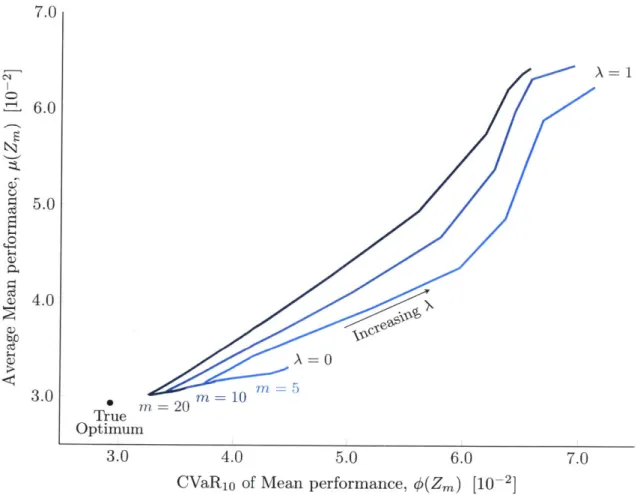
all realizations, pt(Zm), and the CVaRi₀ in mean performance between realizations, < (Zm) (see Eqn. 2.16). These mean-risk trade-off curves are shown in Figure 2-8.

7.0

L 6.0

5.0 Ce 4.0

3.0

3.0 m =0 10 M= 5 True m =20 Optimum 3.0 4.0 5.0 6.0 7.0

CVaR_{1 0 of Mean performance, <(Zm) [10-2]}

Figure 2-8: Mean versus CVaR_{10 curves generated using MOO, with varying sample} size, for the acoustic horn design problem. Each curve corresponds to a sample size m = _{5, 10, 20, and is computed by averaging over T = 1000, 600,200 samples,}

respectively. Each point on a curve corresponds to a particular value of A

e

[ 0, 1 ].

We see that increasing A from zero (i.e., adding some importance to the variability objective) improves both the average and CVaR_{10 in performance over repeated trials.} In particular, we see that if the optimal value of A is chosen for a sample size m =

5, the average performance of the resulting designs is better than a sample of size m = _{10 with A = 0. Similarly, samples of size m = 10 with the optimal A parameter}

outperform samples of size m = 20 with A = _{0. This suggests that introducing a}

variance reduction objective and optimally selecting the trade-off parameter A can result in an improvement in the mean performance of designs, in terms of both the

average and CVaR_{1 0} over many sample realizations.

However, increasing A past a critical value leads to a sharp reduction in the average

this trend more concretely, we revisit the sample realizations studied in Figure 2-6.

Recall that these so-called best and worst realizations produced the best and worst

performing designs (respectively) using the SAA approach. Figure 2-9 shows the

performance of horn designs found by solving M for A

0, 0.5, and 0.95, using the

worst case sample of size m

5.

14.0

0

12.0

L 10.0

01

8.0

Sample Realization

8.0

3

6.0

0

13

4.0

2.0

0.0

1.3

1.4

1.5

Uncertain parameter, u

Figure 2-9: Performance over the uncertainty space, LU, of designs computed by

solving M(A), with A = 0,0.5,0.95 and the worst-case sample of size m

=

5

realiza-tions.

Recall that in the A

=

0 case, M reduces to 8 and the designer optimizes for

mean performance at the realized uncertainty values. The resulting design in this

case exhibits good performance in the sampled region of the uncertainty space, but

poor performance in the region where the uncertain parameter was not realized in

the sample (in this case near u

=

1.3). In this way, the design has been over-fit to

the sample. Adding weight to the variance reduction objective gives the A

=

0.5

sign. This design exhibits worse performance at some realized values of the uncertain

parameter, but in return exhibits more consistent performance over the uncertainty

space. The net effect is that this design has improved mean performance under the

true distribution of uncertainty, despite having worse mean performance under the

sample distribution. However, we see that as A is increased further to A

=

0.95,

the mean performance under the true distribution suffers, as the variance reduction

objective dominates and leads to consistent, but consistently poor performance.

Figure 2-10 gives a plot analogous to Figure 2-9, this time showing the performance

of designs found using the best possible sample of size m

=

5 studied in the previous

section.

14.0

12.0

10.0

Sample Realization

8.0

A =0.95

2

6.0

0

z

4.0

2.0

0.0

1.3

1.4

1.5

Uncertain parameter, u

Figure 2-10: Performance over the uncertainty space U of designs computed using

A

=

0,0.5,0.95 and the best-case sample of size m

=

5 realizations of the uncertain

parameter.

In this case, adding weight to the variance reduction objective by increasing A

always degrades design performance under the true distribution. However, this

re-duction is minor at moderate values of A, e.g., in the A

=

0.5 case shown. This

suggests that while the variance reduction objective may be beneficial to design

per-formance when optimizing with a poor sample, it may also harm perper-formance when

a favorable sample is used.

From these results, we can conclude that adding a variance reduction objective

makes the design methodology robust to poor realizations of the sample. This

ro-bustness is achieved by ensuring that the designs we select are able to generalize from

the sample distribution to the true distribution. However, a criticism of the MOO

approach is that the variance reduction objective does not directly robustify designs

against partial information. Instead, it results in designs that are generally

conserva-tive, performing consistently at the cost of performing well on average. In particular,

if the designer increases A past a critical value the design will become overly

conser-vative, leading to consistently poor design performance. Note that this critical value

is not known to the designer a priori. Moreover, it depends on the particular

realiza-tion of the sample used, so there is no way to guarantee that the value of A used in

the optimization does not exceed the critical value. In this way, the addition of the

variance reduction objective can in fact be a threat to mean design performance.

In this section we have illustrated the importance of ensuring that designs are

not over-fitted to the empirical distribution given by a random sample. This

natu-rally raises the question of whether we can explicitly seek such designs, rather than

achieving this feature as a secondary effect of variance reduction.

CHAPTER 3

DISTRIBUTIONALLY ROBUST DESIGN

OPTIMIZATION

In this section we present a principled method for introducing the notion of robust-ness against variability in sample distributions into the design problem, using the mathematical framework of distributionally robust optimization (DRO). Section 3.1 formulates the problem of finding distributionally robust designs from a given sample of the uncertain parameters. These are designs that achieve good mean performance under the sample distribution, while requiring that this performance be robust to deviations in the distribution of the uncertainty. Section 3.2 discusses how to select a set of probability distributions to robustify the design against, and presents efficient algorithms for solving the resulting distributionally robust design problem.

3.1

Formulation

The central idea behind the distributionally robust approach is to optimize the de-sign while considering a set of possible distributions of the uncertainty, rather than a single distribution.132 3

The set of distributions that we consider in the optimiza-tion is termed the ambiguity set,'4 which we denote by P. We seek a design that performs well for all distributions within the ambiguity set. This is achieved by solv-ing a minimax problem to optimize the worst-case expected performance under any distribution within the ambiguity set. Using the notation introduced in Chapter 2.1,

the distributionally robust design optimization problem can be written

minmax

EP

{Q

(x, u)],

(3.1)

xEX PEP

where P E P denotes probability distributions within the ambiguity set P. In the setting we consider, the designer has access to a sample of m independent realizations

of u, randomly drawn from Pu and denoted u1,..., um.,. This sample is used to

compute the expectation in the DRO problem (Eqn. 3.1), giving the finite sample DRO problem

m

minmax ZiE Q(x,u). (3.2) XCX pEP i=1

We denote the optimal design found in D by xm, where the ambiguity set used in

the optimization, P, will be clear from the context, or explicitly denoted using the notation xmIp. Solving 'D does not require knowledge of the true distribution of uncertainty. Instead it requires the designer to specify the ambiguity set, which is assumed to contain the true distribution with high probability.

The inner maximization problem in D involves finding the worst-case expectation over all distributions in this ambiguity set. This inner maximization problem gives the worst-case distribution

m

p* = argmax Ep [Q (x, u)] = argmax PiQ(x, uj). (3.3)

PEP PEP .

Note that in the context we consider, the ambiguity set contains only discrete prob-ability distributions, which we denote p (c.f. P for a general distribution). This ensures that computing the expectation under any distribution in the ambiguity set is tractable given only a black-box computational model. Once the worst case dis-tribution p* is found, the outer minimization problem finds the design that achieves the best possible improvement in the mean performance under this distribution. This outer problem now has the same form as the SAA problem, 8 (Eqn. 2.2), with the worst-case distribution p* taking the place of the empirical distribution

p,

and can be solved using similar optimization methods. A noteworthy difference however, is

44

,-that the worst-case distribution within the ambiguity set may differ between designs. Thus if an iterative design optimization method is used, the inner optimization needs to be re-solved at each iteration. Furthermore, it is also worth noting that if the worst-case distribution p* is allowed to have many zero entries-as is the case when an L2-norm ambiguity set is used (see Section 3.2.1)-then the outer optimization

problem can become poorly conditioned, and will consequently be sensitive to the initial condition. For the acoustic horn design problem, we are able to overcome this challenge by switching from an interior-point method to a trust-region reflective algorithma.

Finally, it is interesting to note that in contrast with the MOO problem, M (Eqn. 2.17), we are not explicitly optimizing for a reduction in the variation in perfor-mance over the uncertainty space. In Section 2.3 we showed that adding a variance reduction objective to the problem does make the resulting designs robust to changes in the distribution of uncertainty. However, we also showed that this can come at the cost of over-conservatism, with the resulting designs often exhibiting consistently poor performance. In the DRO approach we only explicitly optimize for mean per-formance. We introduce robustness by optimizing for mean performance under all distributions within the ambiguity set. This requirement prevents the optimization from over-fitting the design to a single distribution that, under partial observability, is likely to differ from the true distribution. The DRO formulation often implicitly reduces the variation in performance over the uncertainty space, but more impor-tantly, it guarantees that the resulting design is robust to deviations in the uncertain distribution. The challenge of DRO lies in selecting the ambiguity set, and computing the worst-case distribution in a computationally efficient manner.