HAL Id: hal-03040254
https://hal.archives-ouvertes.fr/hal-03040254
Submitted on 4 Dec 2020
HAL is a multi-disciplinary open access
archive for the deposit and dissemination of
sci-entific research documents, whether they are
pub-lished or not. The documents may come from
teaching and research institutions in France or
abroad, or from public or private research centers.
L’archive ouverte pluridisciplinaire HAL, est
destinée au dépôt et à la diffusion de documents
scientifiques de niveau recherche, publiés ou non,
émanant des établissements d’enseignement et de
recherche français ou étrangers, des laboratoires
publics ou privés.
Multi-Carrier Reflectometry for Distributed Diagnosis
in Complex Wired Networks
Ousama Osman, Soumaya Sallem, Laurent Sommervogel, Marc Olivas
Carrion, Pierre Bonnet, Francoise Paladian
To cite this version:
Ousama Osman, Soumaya Sallem, Laurent Sommervogel, Marc Olivas Carrion, Pierre Bonnet, et al..
Sensor Communication Implementation Using Multi-Carrier Reflectometry for Distributed
Diagno-sis in Complex Wired Networks. IEEE Transactions on Electromagnetic Compatibility, Institute of
Electrical and Electronics Engineers, 2020, pp.1-10. �10.1109/TEMC.2020.3034175�. �hal-03040254�
0018-9464 © 2015 IEEE. Personal use is permitted, but republication/redistribution requires IEEE permission. See http://www.ieee.org/publications_standards/publications/rights/index.html for more information.
Sensor Communication Implementation Using Multi-Carrier
Reflectometry for Distributed Diagnosis in Complex Wired Networks
Ousama Osman, Student Member IEEE, Soumaya Sallem, Laurent Sommervogel,
Marc Olivas Carrion, Pierre Bonnet and Francoise Paladian
Abstract— This paper presents the integration of sensor communication using the diagnosis signal of wired networks. In order to cover the entire network, the diagnosis of branched networks requires the use of distributed diagnosis systems. The objective of this paper is to propose a novel technique of ensuring efficient communication between distributed reflectometers (sensors) by using the transmitted part of the Multi-Carrier Time Domain Reflectometry (MCTDR) signal. Our approach provides unambiguous fault location thanks to sensor data sharing and fusion, which improves the accuracy of fault location and the quality of the diagnosis. MCTDR has already been proven as an efficient method for online diagnosis by enabling precise bandwidth control while avoiding interferences. The main novelty of our technique is to inject an MCTDR signal carrying information which is capable of ensuring network diagnosis and reliable communication between several distributed sensors at the same time. This is done by exploiting, simultaneously, both the transmitted part and the reflected part of the MCTDR signal. The effectiveness of the proposed approach is evaluated by a series of simulations and experiments (based on field-programmable gate array (FPGA) implementation) on different types of cables and with different configurations.
Index Terms—Reflectometry, MCTDR, wire diagnosis,
distributed diagnosis, data fusion, sensor communication. I. INTRODUCTION
Over the last few decades, there has been tremendous progress in the efforts to move towards electric means of transport (electric vehicles, more electric aircraft, etc.). This has caused an increase in both the lengths of the cables and the complexity of wired networks. Accordingly, wire diagnoses have become essential for ensuring safety, security, and in particular, electromagnetic compatibility (EMC) performance [1].
Electrical cables are highly exposed to both internal and external conditions, such as humidity, corrosion, local heating, aging, and mechanical damage that can create defects. This, in turn, can result in the degradation of the cable shield and, as a consequence, dramatically change the emissivity and the susceptibility of electrical equipment. Accordingly, the EMC issues related to faulty electrical wiring have encouraged many
researchers to look for novel solutions and techniques [2]-[5], which would be capable of accurately locating the faults in wired networks. Much of the research is based on reflectometry [6] techniques, where high-frequency test signals are injected down a network under test (NUT), in order to observe the reflections returned from each impedance discontinuity (such as junctions and faults). The correlation of the reflected signal to the injected one is known as a reflectogram, whose analysis provides information about the presence, location, and type of the discontinuity detected.
The reflectometry methods are classified into three main families: Time Domain Reflectometry (TDR) [7], [8], Frequency Domain Reflectometry (FDR) [9], [10] and Time-Frequency Domain Reflectometry (TFDR) [11], [12]. They show great performance in detecting hard faults (open or short circuits) but they start failing when it comes to soft faults (cracks, insulation damages, etc.) [13]. In fact, soft faults are characterized by a local change of the wire properties which can produce weak echoes that are difficult to detect. Therefore, it is imperative to be able to detect them early before they become hard faults.
Currently, live monitoring of wired networks is needed i.e. while the target system is in normal operation. Specific methods have been designed for online diagnosis, such as Spread Spectrum-TDR (SSTDR) [14], Noise Domain Reflectometry (NDR) [15], Multi-Carrier Reflectometry (MCR) [16] and its variants Multi-Carrier TDR (MCTDR) [17] and Orthogonal Multi-Tone TDR (OMTDR) [18]. These methods have shown promising and efficient results in detecting and locating cable faults without interfering with useful signals.
However, during propagation through the wiring system, the effectiveness of these methods is impeded by the signal loss caused by degradation [19]. This phenomenon becomes more complex in branched networks due to the multiple reflections caused by multiple junctions, faults, etc. In such cases, distributed reflectometry is required [20], [21], where several sensors are placed at strategic points on the network, which maximizes the diagnosis coverage and eliminates fault location ambiguities. But as multiple sensors are taking measurements simultaneously, specific processing methods are required to avoid interference noise between concurrent sensors [22].
In the context of distributed diagnosis, the communication between different sensors is essential, to allow data fusion to make a decision about the fault location. Recently, sensor communication based on the OMTDR method has been proposed [23]. OMTDR has shown promising results in online
This work was supported by WiN-MS (Wire Network Monitoring Solutions) company within the framework of PhD thesis (CIFRE contract).
O. Osman, S. Sallem, L. Sommervogel and M. O. Carrion: WiN-MS, 503, rue de Belvédère, 91400, Orsay, France (e-mail: [email protected]).
P. Bonnet and F. Paladian : Université Clermont Auvergne, CNRS, SIGMA Clermont, Institut Pascal, F-63000 CLERMONT-FERRAND, FRANCE (e-mail : [email protected], [email protected]).
diagnosis of simple and complex topologies. However, the main drawback of OMTDR becomes evident in the presence of side lobes around the central lobe, which can cause fault detection problems (false alarms). This requires a specific filtering window which is costly in terms of computing time and which can hide defects, particularly in complex networks. Furthermore, to ensure the communication between sensors, the OMTDR uses the OFDM (Orthogonal Frequency Division Multiplexing) technique as a base, which also requires a complex post-processing phase of the different blocks of the OFDM method.
The objective of this article is to propose a new distributed diagnosis technique called communication-MCTDR (C-MCTDR), which enables communication between sensors using the subcarrier phases of the MCTDR signal [24]. The main novelty is to simultaneously exploit the transmitted part of the MCTDR signal for communication and the reflected part for diagnosis. The integration of this type of sensor communication enables data fusion between distributed sensors, as well as an in-depth diagnosis of the network without ambiguity.
The proposed method, based on the MCTDR signal, presents considerable advantages in comparison with other techniques. These include good autocorrelation properties that provide good performance (faults detection and location) on distributed diagnosis, complete bandwidth control, and online diagnosis without interference. More importantly, C-MCTDR adds the communication between distributed sensors to accurately determine the position of faults in a branched network. Embedding all these advantages in a smart diagnosis system would be very effective for real-time diagnosis of future wired networks as they could perform self-diagnoses.
The paper is organized as follows. Section II presents the numerical model that describes the propagation of the wave along the lines of a network. Section III recalls the MCTDR principle and introduces mathematical models of the proposed sensor communication method. Section IV discusses the proposed distributed diagnosis strategy using our C-MCTDR method. Section V presents simulation and experimental results to validate the feasibility of the proposed approach. The results showing method robustness are presented in section VI. The last section concludes the paper.
II. THE TRANSMISSION LINE PROPAGATION MODEL
Many authors [25], [26], rely on the 4-parameter RLCG model (resistance, inductance, capacitance, and conductance per unit length), from which the well-known telegrapher’s equations [27] are derived, to describe the propagation of a wave along a cable. These equations describe the evolution of voltage and current along the cable as functions of the RLCG parameters. Based on this model, the characteristic impedance as a function of the angular frequency ω is defined as follows:
𝑍𝑐(𝜔) = √
𝑅 + 𝑗𝐿𝜔
𝐺 + 𝑗𝐶𝜔 (1)
and the propagation constant 𝛾 (radians/m) as well:
𝛾(𝜔) = √(𝑅 + 𝑗𝐿𝜔)(𝐺 + 𝑗𝐶𝜔) = 𝛼(𝜔) + 𝑗𝛽(𝜔) (2) where 𝛼 is the attenuation constant (nepers/m) and 𝛽 is the phase constant (radians/m).
Finally, if there is an impedance change along the line (e.g., from 𝑍𝑐1 to 𝑍𝑐2), the associated reflection coefficient is
obtained as follows:
Г =𝑍𝑐2− 𝑍𝑐1 𝑍𝑐2+ 𝑍𝑐1
(3) This reflection coefficient can be located as follows:
𝑑 = 𝜏. 𝑣𝑝(𝜔)/2, with 𝑣𝑝(𝜔) = 𝜔/𝛽(𝜔) (4)
where 𝜏 represents the measurement of the round-trip time (RTT) between the injection point and the impedance discontinuity, 𝑣𝑝 is the propagation speed through the cable.
The signal propagation through the complex NUT is modeled as in [28], to provide its corresponding reflectometry response. The numerical simulations were performed thanks to an in-house code solving telegrapher’s equation in the frequency domain. Taking into account the attenuation and the dispersion phenomenon [29], the RLCG parameters take the following form in the simulation code:
𝑅 = 𝑅0√𝑓 and 𝐺 = 𝐺0𝑓
𝐿 = 𝐿0+ 𝑅0/(2𝜋√𝑓) and 𝐶 = 𝐶0
(5) Two types of cable were used for the experiment: Coaxial cable (RG-58) and twisted pair cable (CVZ). The values of 𝑅0, 𝐿0, 𝐶0 and 𝐺0 are presented in Table 1.
Table 1. The cable parameters used for experiments.
Cable family 𝑅0 (µΩ/𝑚) 𝐿0 (𝑛𝐻/𝑚) 𝐶0 (𝑝𝐹/𝑚) 𝐺0 (𝑝𝑆/𝑚) RG-58 130 250 100 0.8 CVZ 80 596 97 0.24
III. MCTDR THEORY: FAULT DIAGNOSIS AND SENSOR COMMUNICATION
A. MCTDR reflectometry
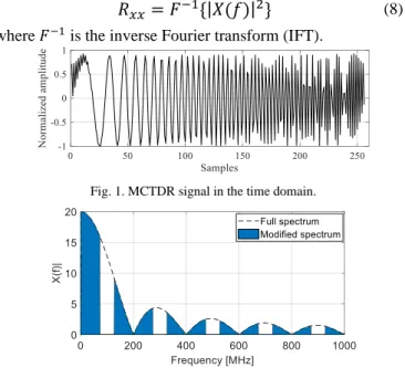
Based on the multi-carrier principle, MCTDR [17] models the injected test signal as a sum of a finite number of sinusoids to enable a precise control of the spectrum. The test signal is defined by: 𝑥𝑛= 2 √𝑁∑ 𝑐𝑘cos ( 𝑁/2 𝑘=0 2𝜋𝑘 𝑁 𝑛 + 𝜃𝑘 ) (6) where 𝑐𝑘 and 𝜃𝑘 represent the amplitude and the phase of the
subcarrier 𝑘, respectively. 𝑁 is the carrier number, with n being the sampling index. Fig. 1 shows the shape of the MCTDR signal in the time domain.
Its Fourier transform (FT), with a digital system operating at the sampling frequency 𝑓𝑠= 1/𝑇𝑠 and digital to analog converter
|𝑋(𝑓)| = |𝑠𝑖𝑛𝑐(𝜋𝑓𝑇𝑠)|. ∑ 𝑐𝑘 𝑁/2 𝑘=1 ∑ +∞ 𝑛=−∞ [δ (𝑓 − (𝑘 𝑁+ 𝑛) 𝑓𝑠) − δ (𝑓 + (𝑘 𝑁− 𝑛) 𝑓𝑠)] (7)
In addition, the MCTDR signal has good autocorrelation properties that enable accurate fault location. Fig. 2 represents the |𝑋(𝑓)| as a function of frequency and Fig. 3 shows the autocorrelation of the injected signal which is obtained as follows:
𝑅
𝑥𝑥= 𝐹
−1{|𝑋(𝑓)|
2}
(8)where 𝐹−1 is the inverse Fourier transform (IFT).
Fig. 1. MCTDR signal in the time domain.
Fig. 2. MCTDR signal spectrum with 𝑁 = 256, 𝑓𝑠= 200 𝑀𝐻𝑧 and 𝑐𝑘= 0
for 𝑘 ∈ 95, … , 128.
Fig. 3. Autocorrelation function of the MCTDR signal.
To avoid any interference problems during online diagnosis, the subcarrier frequencies of the MCTDR signal would have to be selected outside the frequency bands of the useful signals and the EMC (Electromagnetic Compatibility) spectrum involved. This can be overcome by canceling or reducing the amplitude 𝑐𝑘 of the signal spectrum leading to bandwidth
control. This is done for the frequency bands lying within the operational bands of the system. Canceling 𝑐𝑘 can cause a loss
of information that degrades the autocorrelation function of the test signal. Fig. 3 shows the autocorrelation of the MCTDR signal in two cases: (1) the sensor uses all the available bandwidth, and (2) a set of available bandwidth spectra is canceled. The latter case leads to the appearance of several
secondary lobes around the main lobe (Fig. 3 (blue)), which can mask soft fault echoes in the reflectometry response. Therefore, a specific filtering window (Hamming, Dolph-Chebyshev, etc.) is required to eliminate these secondary lobes.
B. Analytic models: Frequency analysis of MCTDR signal
To evaluate the communication between two sensors, it is the transmitted part of the test signal, after it has passed through the cable, that is of interest. The cable transfer function 𝐻(𝑓) is given by:
𝐻(𝑓) = ∏ (1 − Г𝑖)𝑒−𝛾(𝑓)𝑙
𝑖 (9)
where 𝑙 is the cable length, (Г𝑖) 𝑖>0 represents the reflection
coefficients of the impedance discontinuities.
The proposed technique (described in Section IV) is based on the use of the subcarrier phases (𝜃𝑘) of the MCTDR signal
to encode messages. These phases are defined by applying a digital modulation technique. Each phase represents a symbol of digital information sent by the transmitter sensor. For simplicity, only positive frequencies of the MCTDR signal are used in the analytical model. The received signal (at the receiver sensor), following the injection of the MCTDR signal into the cable, is given by:
𝑌(𝑓) = 𝑋(𝑓)𝐻(𝑓) = 𝑠𝑖𝑛𝑐(𝜋𝑓𝑇𝑠) ∑ ∑ 𝑐𝑘𝑒𝑗𝜃𝑘 𝑁−1 𝑘=0 𝑃−1 𝑛=0 δ (𝑓 − (𝑘 𝑁+ 𝑛) 𝑓𝑠) . ∏ (1 − Г𝑖)𝑒 −𝛾(𝑓)𝑙 𝑖,𝑗 = 𝑠𝑖𝑛𝑐(𝜋𝑓𝑇𝑠)𝑒−𝛼𝑙∏ (1 − Г𝑖) 𝑖 ∑ ∑ 𝑐𝑘𝑒 𝑗(𝜃𝑘−𝛽𝑙) 𝑁−1 𝑘=0 𝑃−1 𝑛=0 δ (𝑓 − (𝑘 𝑁+ 𝑛) 𝑓𝑠) (10)
where P represents the number of lobes of the MCTDR spectrum. The transmitted phase sequence (𝜃𝑘) is recovered on
the main lobe (𝑃 = 1) of the MCTDR spectrum which contains most of the energy. The phase of this signal is given by:
𝑎𝑟𝑔(𝑌(𝑓)) = −𝛽(𝑓)𝑙 + ∑ 𝜃𝑘𝛿 (𝑓 − 𝑘 𝑁𝑓𝑠) 𝑁−1 𝑘=0 (11) At reception, the receiver sensor must calculate the N phases (𝜃𝑘) from 𝑌(𝑓). We note that the phase of 𝑌(𝑓) depends on the
parameters of the cable 𝛽(𝑓) and 𝑙. The received signal phase on each carrier frequency band also needs to be calculated. The estimation sequence phase is done in two steps:
To begin, we take a first measurement (𝑌0) by sending a
sequence of zero phases: {𝜃𝑘} = {0}.
𝑎𝑟𝑔(𝑌0(𝑓)) = −𝛽(f)𝑙 (12)
In a second step, we transmit a message on the sequence of the phases {𝜃𝑘}. Then, the receiver estimates the sent sequence:
𝜃𝑘𝑒𝑠𝑡= (𝑝ℎ𝑎𝑠𝑒(𝑌(𝑓)) − 𝑝ℎ𝑎𝑠𝑒(𝑌0(𝑓))). ∏ (𝑓)
𝑘 (13)
where ∏𝑘(𝑓) is a matched filter used to select the frequency band corresponding to the sub-carrier number k.
∏ (𝑓) 𝑘 = {1 𝑖𝑓 𝑓 = ( 𝑘 𝑁+ 𝑛) 𝑓𝑠 0 𝑒𝑙𝑠𝑤ℎ𝑒𝑟𝑒 (14)
IV. COMMUNICATION USING C-MCTDR
The block diagram in Fig. 4 illustrates the different steps followed by the C-MCTDR method from the generation of the test signal, its injection into the NUT, to the construction of the reflectogram for diagnosis or phase demodulation for communication. The C-MCTDR signal is composed of N subcarriers represented by the vector 𝑆𝑘 = 𝑐𝑘𝑒𝑗𝜃𝑘, with 𝜃𝑘= 𝑖2𝜋
𝑀 where M is the phase mapping order, and 𝑖 is a parameter
taking any value between 0 and 𝑀 − 1. The subcarrier phases are generated by applying M-PSK (phase shift keying) mapping. The amplitude of each symbol is controlled by the coefficient 𝑐𝑘 which allows the control of the signal spectrum.
The subcarriers must then be distributed, as per the Hermitian symmetry, to generate a real signal [30]. After that, an inverse fast-Fourier transform (IFFT) is applied to transform the multi-carrier signals into the time domain. After the Digital-to-Analog Converter (DAC), the multi-carrier signal, denoted 𝑥(𝑡), is injected into the NUT. This signal propagates through the NUT and reflects back to the injection point when it crosses impedance discontinuities such as a fault. Fig. 5 shows a typical C-MCTDR test signal in the time domain composed of 𝑁 = 256 subcarriers (𝑐𝑘 = 1 for 𝑘 ∈ 1, … , 256). The total available
bandwidth is [0-200 MHz], the frequency space between two consecutive subcarriers is fixed at 781.25 kHz.
Fig. 4. Block diagram of C-MCTDR Principle.
Fig. 5. C-MCTDR test signal in the time domain composed of 𝑁 = 256 sub-carriers (𝑐𝑘= 1 for 𝑘 ∈ 1, … , 256).
Accordingly, the reflected signal is expressed as follows: 𝑦(𝑡) = 𝑥(𝑡) ∗ ℎ(𝑡) + 𝑛(𝑡) (15)
where * is the convolution product, ℎ(𝑡) represents the response of the NUT, and 𝑛(𝑡) is the channel noise.
The reflected signal 𝑦(𝑡) is sampled by an Analog-to-Digital Converter (ADC) to produce the discrete signal 𝑦(𝑛). The noise
distribution associated with the measurements is assumed to be white and Gaussian. Then, an averaging step over 𝑁 measurements (𝑁 = 32) is performed in order to increase the signal-to-noise ratio (SNR), thus improving the measurement accuracy. The averaging step is performed as follows:
𝑦̂ =1 𝑁∑ 𝑦 (𝑛) 𝑁−1 𝑛=0 (16) Each sensor then performs a post-processing step that can provide two functions: sensor diagnosis and sensor communication. For the first function, the correlation module computes the cross-correlation function between the injected signal and the reflected signal. This is plotted to build a
reflectogram whose post-processing analysis allows for the
precise location of any faults in the NUT.
The second function enables the exchange of information between sensors, where the receiver performs the reverse process of the transmitter to retrieve the sent message. The measured samples (in the frequency domain) are shifted to the correct position to compensate for the delay between the transmitter and receiver sensors. The received bits are then extracted from the set of subcarriers by phase demapping.
V. C-MCTDRMETHODOLOGY:DIAGNOSIS AND
COMMUNICATION
A. Diagnosis procedure in a complex network
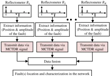
In a complex network, several sensors are needed for better coverage of the entire network. Fig. 6 summarizes the steps followed to locate and characterize the fault in a branched network.
Fig. 6. Diagnosis procedure in wired networks.
First, each reflectometer 𝑅𝑘 k ∈ {1, 2, … , 𝑁}, 𝑁 is the
number of reflectometers, performs the reflectometry measurement and builds its own reflectogram. The reflectogram is further post-processed to identify the fault. Each reflectometer then uses the phases of the MCTDR signal to
𝑆𝑘= 𝑐𝑘𝑒𝑗𝜃𝑘 IFFT Wired network 𝑥𝑘(𝑡) ∗ ℎ𝑘(𝑡) + 𝑛𝑘(𝑡) Averaging 1 𝑁∑ 𝑦 (𝑛) 𝑁−1 𝑛=0 FFT Post-processing IFFT phase demapping 𝑠 y(t) ADC DAC 𝑆𝐹 𝑋∗(𝑓) 𝑌(𝑓) 𝑥(𝑡) 𝑦(𝑛) conj. × defect received data Reflectogram Correlation Communication Г𝑥𝑦(𝑛) Hermitian symmetry 𝜃 𝑐 C-MCTDR Signal 𝑦̂
Reflectometer 𝑅1 Reflectometer 𝑅2 Reflectometer 𝑅𝑁
Fault(s) location and characterization in the network Transmit data via
MCTDR signal
Transmit data via MCTDR signal
Data fusion Transmit data via
MCTDR signal Extract information (Position & amplitude
of the fault)
Extract information (Position & amplitude
of the fault)
Extract information (Position & amplitude
transmit the useful data (such as fault location, amplitude, ambiguous branches, etc.) to a main reflectometer or central data-processing unit. The relevant data are encapsulated into data frames managed by a communication protocol. Finally, the main reflectometer analyzes the collected results and applies data fusion, thus facilitating the decision-making pertaining to the location and to the characterization of the fault.
B. Sensor placement optimization
For an efficient and pertinent diagnosis, the number and location of the sensors must be optimized so as not to affect the quality of the diagnosis [31]. For better coverage, the sensors should be placed at strategic points on the network. In order to reduce the number of sensors, the authors in [32] have proposed the implementation of 𝑁𝑠𝑒𝑛𝑠𝑜𝑟 sensors in a complex network:
𝑁𝑠𝑒𝑛𝑠𝑜𝑟= ∑(𝑛𝑗− 1) 𝐽−1
𝑗=0
(17) where 𝐽 is the total number of junctions in the network and 𝑛𝑗
is the number of branches at the 𝑗𝑡ℎ junction. Moreover, to
optimize the placement of the sensors, it is generally recommended to place them at the ends of the shortest lines, as they can provide more accurate information about any faults occurring after a junction.
C. C-MCTDR signal applied to a complex network
The considered double Y-junction network illustrated in Fig. 7 was implemented using 50 Ω coaxial cables. The network is diagnosed by two reflectometers 𝑅1 and 𝑅2. Each can perform
two functions: network diagnosis and data communication. The reflectometers and the branches are adapted to the impedance of the network (𝑍𝐿= 𝑍𝑐 = 50Ω) to avoid reflections and
multiple paths. The branch 𝐵3 is affected by a chafing soft fault
(Fig. 8) at 5.5 m from 𝑅1. It is identified by a localized change
of characteristic impedance, with a length of ∆𝐿 = 3 𝑐𝑚, and an impedance 𝑍𝑑= 𝑍𝑐(1 + Zc) (∆𝑍𝑐 = 25%). In order to
evaluate experimentally the impedance variation of the created soft fault, we relied on the theorical and numerical model that can provide information on the fault echo. Thus, the insulation was progressively destroyed until the correct echo of the simulated fault was found.
Fig. 7. Topology of the NUT used to test and validate the proposed C-MCTDR communication based reflectometry.
The proposed C-MCTDR Diagnosis/Communication approach presented in Fig. 4 was implemented on a specific sensor (output signal < 1 V, impedance 50 Ω). The sensor embeds a field-programmable gate array (FPGA) that provides synchronous clocks to drive an injection unit (14-bit DAC) with an acquisition unit (12-bit ADC). The DAC sampling frequency
is 𝐹𝐷𝐴𝐶= 200 MHz and the ADC sampling frequency is
𝐹𝐴𝐷𝐶= 100 MHz. The acquisition resolution is improved
through a pseudo-oversampling which is achieved by increasing the phase of the ADC sampling clock using a constant phase shift. This improves the fault location accuracy.
Fig. 8. Chafing soft fault (chafing of the shield and the insulator) created on the RG-58 coaxial cable.
A graphical user interface (GUI) controls the injection/acquisition procedure of the diagnosis signal. This GUI runs on an Android/Windows platform using menus and other visual indicators and graphical representations that show the results of the communication, and the analysis, pertaining to the status of the network (reflectogram display). Each reflectometer has wireless communication features capable of sending information to the GUI. What is more, the distributed reflectometers can communicate with each other and share information thanks to the C-MCTDR signal.
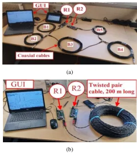
In order to validate the performance of the proposed approach, experimental tests were conducted with the complex structure depicted in Fig. 7. Standard 50 Ω coaxial cables were used for the transmission lines making up the NUT: the resulting system is shown in Fig. 9 (a).
(a)
(b)
Fig. 9. (a) Implementation of the NUT of Fig. 7 using coaxial cables and connected to the reflectometers 𝑅1 and 𝑅2 to perform the C-MCTDR
meausurements . (b) A twisted pair cable connected to 𝑅1 and 𝑅2.
D. Sensor diagnosis function using C-MCTDR
The reflectometers 𝑅1 and 𝑅2 injected the test signal 𝑥(𝑡)
into the NUT shown in Fig. 7. The channel impulse response ℎ(𝑡) is expressed as: ℎ(𝑡) = ∫ Г0(𝑓) +∞ −∞ 𝑒𝑗2𝜋𝑓𝑡𝑑𝑓 (18) 𝐵1 (3𝑚) message j 𝐵2 (3𝑚) 𝐵4 (10𝑚) 𝐵3 (10𝑚) 𝐵5 (5𝑚) 50Ω 50Ω Г0 Г1 message i 𝑅1 𝑅2 5.5 𝑚 Chafing soft fault 𝐽1 𝐽2
Г0(𝑓) is the reflection coefficient equivalent to the whole NUT,
its equation is given by:
𝛤0(𝑓) = 𝛤1𝑒(−2 𝛾(𝑓)𝑙1) (19)
where 𝛾 is the propagation constant and 𝑙1 is the length of the
line 𝐵1. The reflection coefficient 𝛤1, equivalent to the whole
NUT, except the line 𝐵1, is given as follows [28]:
𝛤1=
−1 + 𝛤2 𝛤3+ 𝛤3 𝛤4+ 𝛤2 𝛤4+ 2 𝛤2 𝛤3 𝛤4
2 + 𝛤2+ 𝛤3+ 𝛤4− 𝛤2 𝛤3 𝛤4
(20) A C-MCTDR signal, composed of 𝑁 = 256 subcarriers, was generated (Fig. 5) and injected into the NUT to perform both the diagnosis and the communication functions.
Fig. 10 and Fig. 11 show the simulated reflectograms of the implemented network shown in Fig. 7. The first peak (distance =0) is the mismatch between the reflectometer and the network. The second negative peak corresponds to the junction 𝐽1. Then,
the soft fault generated a small variation in the reflectogram that was detected at 5.5 m from 𝑅1. As this fault could be located on
either the branch 𝐵2 or on the branch 𝐵3, a fault location
ambiguity was observed. As for the 𝑅2, it located the soft fault
at 12.5 m (Fig. 11), it could also be located on either the branch 𝐵3 or on 𝐵4. Here, a fault location ambiguity was also
identified. In short, 𝐵2, 𝐵3 and 𝐵4 are the ambiguous branches
on which the soft fault could be located. Accordingly, the data fusion between 𝑅1 and 𝑅2 is necessary to accurately locate and
characterize the soft fault.
Fig. 10. Reflectograms of the faulty network obtained by reflectometer 𝑅1.
Fig. 11. Reflectograms of the faulty network obtained by reflectometer 𝑅2. Fig. 12 and Fig. 13 show the measured reflectometry responses (reflectogram) of the healthy network by the
reflectometers 𝑅1 and 𝑅2, respectively. They show a
comparison between the response of the MCTDR signal and the C-MCTDR signal, illustrating that both signals are in good agreement in terms of the position and amplitude of the main peaks. In fact, the difference between the two signals depends on the way the subcarrier phases are generated. For the MCTDR signal, they are selected to minimize the Peak to Average Power Ratio (PAPR) in the time domain. This is achieved by the Schroeder method [33] which generates a chirp-like signal as shown in Fig. 1. The phases of the C-MCTDR signal are obtained by M-PSK mapping.
It can be seen in Fig. 12 and Fig. 13 that the reflectometry response is flatter when the phases of the signal are generated by the Schroeder method. This points out that the phase values do not affect the spectrum and the main characteristics of the MCTDR signal.
Fig. 12. Comparison between the response of the MCTDR and C-MCTDR signals for a healthy NUT obtained by the reflectometer 𝑅1.
Fig. 13. Comparison between the response of the MCTDR and C-MCTDR signals for a healthy NUT obtained by the reflectometer 𝑅2. To better illustrate the potential efficiency of the proposed method, a twisted pair cable configuration was considered as shown in Fig. 9 (b), where two sensors (𝑅1 and 𝑅2) were
connected to the ends of the cable to perform the C-MCTDR measurements. Both the sensor diagnosis and the sensor communication function were tested. An open-circuited (𝑍𝐿=
(sensor 𝑅1). The C-MCTDR signal was injected into the cable
on the frequency band from 400 KHz to 10 MHz in order to reduce the attenuation effect of the twisted pair cable. Fig. 14 shows the reflectogram obtained by the sensor 𝑅1 using both
the MCTDR and the C-MCTDR signal. Here, the proposed method detected, and accurately located, the end of the line identified by the reflected echo at 200 m.
Fig. 14. Comparison between the response of the MCTDR and C-MCTDR signals for a twisted pair cable obtained by the reflectometer 𝑅1.
E. Sensor communication function using C-MCTDR
In this section, we look at the communication between sensors using the transmitted part of the C-MCTDR signal. This process enables data exchange between sensors and reduces diagnosis ambiguities in branched networks. We relied on the complex network in Fig. 9 (a) to send messages from 𝑅1 to 𝑅2.
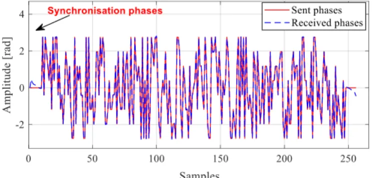
Fig. 15 shows the received C-MCTDR signal (injected by 𝑅1)
in the time domain at the reflectometer 𝑅2. This latter is shifted
to the correct position to compensate for the delay between the transmitter and receiver sensor
Fig. 15. Measured C-MCTDR signal in the time domain by the reflectometer 𝑅2.
The measured signal is sampled at 1 GHz (frequency of the ADC). The acquired oversampled C-MCTDR signal (1 280 samples, the oversampling factor is 10) is composed of 10 sets of samples where each set consists of 128 samples. The higher sampling frequency for the reception allows for better resolution. Then, an average amplitude of each received set of samples is computed in order to find the optimal one. Finally, a reverse process of the oversampling method between the DAC and the ADC is performed in order to find the transmitted phases.
For a C-MCTDR signal composed of 𝑁 = 256 subcarriers and a 8-PSK mapping, the C-MCTDR capacity is given as follows: 𝑁𝑏𝑖𝑡𝑠= (𝑁/2 − 𝑃𝑠𝑦𝑛𝑐ℎ𝑟𝑜) ∗ log28 = 369 (21)
where 𝑁/2 represents the number of useful carriers since the second half of the carriers is obtained by using the Hermitian symmetry to generate a real-valued signal. 𝑃𝑠𝑦𝑛𝑐ℎ𝑟𝑜 represents
the synchronization phases (5 phases are set to zero in our case). In fact, to compensate for the delay between the transmitter and receiver sensors, the frequency domain of the received samples is shifted until we find the values of the 𝑃𝑠𝑦𝑛𝑐ℎ𝑟𝑜 phases
consecutively.
Moreover, by using 8-PSK mapping (3-bits per phase), as well as by averaging the measurements of 32 samples and using oversampling factor of 10, the data transmission rate can be calculated as follows:
𝐷𝑎𝑡𝑎 𝑟𝑎𝑡𝑒 = 𝑁𝑏𝑖𝑡𝑠/(𝑇𝑠∗ 𝑁 ∗ 32 ∗ 10) = 900.88 Kbit/s (22)
Fig. 16 shows the transmission and the reception of 256 phases. The first 5 phases are set to zero for the synchronization step. Then, the bits are extracted from the first 123 received phases by 8-PSK un-mapping.
Fig. 16. A sequence of 256 phases sent by the reflectometer 𝑅1 and received
by the reflectometer 𝑅2. VI. METHODROBUSTNESS
In this section, simulation results are presented to show the bit error rate (BER) performances of the proposed method over a faulty and a noisy channel. The BER is a key parameter used to characterize the quality of the communication channel. It represents the ratio of the number of bit errors to the total number of transmitted bits during a given time interval.
To test the robustness of the proposed method, a white Gaussian noise (⋳𝑌) was added to the received signal, whose
signal-to-noise ratio (SNR) varied from 0 to 50 dB.
𝑌𝑟(𝑓) = 𝑌(𝑓) + ⋳𝑌 (23)
A message of 369 bits was sent on the sequence of the phases of a C-MCTDR signal (𝑁 = 256 sub-carriers), injected into the network of Fig. 7 by the reflectometer 𝑅1 and estimated at the
reflectometer 𝑅2. The 369 bits were modulated using 8-PSK
mapping and then inserted into the C-MCTDR signal as a sequence of 256 phases.
Fig. 17 shows the evolution of the bit error rate as a function of the signal-to-noise ratio in the case of a healthy link between 𝑅1
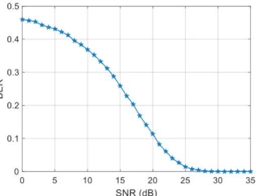
We notice that the same bits are found to be sent in the absence of noise (>30dB).
Fig. 17. Sensor communication: BER performance vs. SNR in the case of a healthy link between 𝑅1 and 𝑅2.
We will now detail the impact of the evolution of the soft fault severity on the communication. In order to simulate a soft fault, a local variation of the characteristic impedance (characterized by a length of 0.4 m and an impedance 𝑍𝑑=
𝑍𝑐(1 +𝑍𝑐) (20% < ∆𝑍𝑐 < 80%)) was simulated on the
branch 𝐵3 of the network (Fig. 7) at 5.5 m from the
reflectometer 𝑅1. In fact, the communication quality is not
affected by soft faults characterized by a length <10 cm and a variation of the characteristic impedance 𝑍𝑐 < 25%, as the C-MCTDR signal phases do not depend on the fault reflection coefficients. A 64-PSK mapping is used in order to increase the data rate. Fig. 18 shows the evolution of the BER as a function of the SNR and according to the variation of the soft fault impedance. It is obvious that the BER increases when the soft fault severity increases. It is also observed that the use of a higher M-PSK is better for high capacity data transmission but that it is easily affected by noise or a faulty channel: with reduced SNR, the BER is lower in the case of 8-PSK than it is in the case of 64-PSK.
Fig. 18. Sensor communication: BER performance vs. SNR, depending on the soft fault characteristic impedance variation (%).
More importantly, the proposed communication method is robust to noise and cable soft faults, especially in the case of low bit rate transmission (8-PSK in our case). The occurrence of a hard fault (open or short circuit) is manifested by the interruption of communication. However, in that case, it can be concluded that there is a problem with the path between the transmitter and the receiver. We note that the BER can also be improved by using an Error Correction Code (ECC) to control
errors in data transmission.
It is equally important to recall that any MCTDR signal is robust to external interferences thanks to the complete control of the spectrum of the injected signal, and also robust to internal interference (between the sensors) thanks to the use of a selective averaging method [22].
VII. CONCLUSION
MCTDR is characterized by its ability to be integrated into an embedded system. Even if MCTDR has shown promising and efficient results in locating cable faults in real-time diagnosis, it is still limited in the case of branched networks. To deal with this difficulty, we have proposed using the subcarrier phases of the MCTDR signal to integrate communication between distributed sensors. This communication ensures data fusion, thus reducing ambiguity and improving the accuracy of fault location in complex networks.
The main contribution of this paper is the notion of the injection of a signal carrying information to perform real-time distributed wire diagnosis and sensor communication. This is done by simultaneously exploiting the transmitted part and the reflected part of the MCTDR signal.
A series of theoretical analysis, simulations, and experiments for different types of cables are presented to demonstrate the effectiveness of the proposed approach. Our future work will focus on the implementation of a communication protocol to achieve the exchange and data fusion between sensors.
ACKNOWLEDGMENTS
The authors would like to thank Mrs. Patricia Mabrut for her careful proofreading.
REFERENCES
[1] M. Kafal, J. Benoit, and C. Layer, “A joint reflectometry-optimization algorithm for mapping the topology of an unknown wire network,” in IEEE SENSORS Conference, pp. 1–3, Nov. 2017.
[2] L. El Sahmarany, L. Berry, N. Ravot, F. Auzanneau, and P. Bonnet, “Time reversal for soft faults diagnosis in wire networks,” Progress in Electromagnetics Research, vol. 31, pp. 45–58, 2013.
[3] M. Kafal, J. Benoit, A. Cozza, and L. Pichon, “A statistical study of dort method for locating soft faults in complex wire networks,” IEEE Transactions on Magnetics, vol. 54, no. 3, pp. 1–4, 2018.
[4] F. Auzanneau, “Wire troubleshooting and diagnosis: review and perspectives,” Prog. Electromagn. Res. B, 49, pp. 253–279, 2013. [5] C. Furse, M. Kafal, R. Razzaghi and Y. June Shin, “Fault Diagnosis for
Electrical Systems and Power Networks: A Review,’ IEEE Sensors Journal, April 2020. DOI: 10.13140/RG.2.2.24213.06882.
[6] C. Furse, Y. C. Chung, C. Lo, P. Pendayala. "A critical comparison of reflectometry methods for location of wiring faults", Journal of Smart Structures and Systems, 2(1), pp. 25-46, 2006.
[7] S. J. P., Time-domain Reflectometry for Monitoring Cable Changes: Feasibility Study. Electric Power Research Institute, 1990.
[8] T.W. Pan, C.W Hsue and J.F Huang, “Time-Domain Reflectometry Using Arbitrary Incident Waveform,” IEEE Transactions on Microwave Theory and Techniques, vol. 50, no. 11, pp. 2558-2563, Nov, 2002.
[9] C. Furse, You Chung Chung, R. Dangol, M. Nielsen, G. Mabey, R. Woodward. "Frequency-domain reflectometry for on-board testing of aging aircraft wiring," IEEE Transaction on Electromagnetic Compatibility 45.2:306-315, May 2003.
[10] Y. C. Chung, C. Furse, and J. Pruitt, “Application of phase detection frequency domain reflectometry for locating faults in an F-18 flight control harness,” IEEE Transaction on Electromagnetic Compatibility, vol. 47, no. 2, pp. 327–334, May 2005.
[11] E. Song et al., “Detection and location of multiple wiring faults via time– frequency-domain reflectometry,” IEEE Transactions on Electromagnetic Compatibility, vol. 51, no. 1, pp. 131–138, Feb. 2009. [12] J. Wang, P. E. C. Stone, D. Coats, Y.-J. Shin, and R. A. Dougal, “Health
monitoring of power cable via joint time-frequency domain reflectometry,” IEEE Transactions on Instrumentation and Measurement, vol. 60, no. 3, pp. 1047–1053, Mars 2011.
[13] L. A. Griffiths, R. Parakh, C. Furse, and B. Baker, “The invisible fray: A critical analysis of the use of reflectometry for fray location,” IEEE Sensors Journal, vol. 6, no. 3, pp. 697–706, 2006.
[14] P. Smith, C. Furse, and J. Gunther, “Analysis of Spread Spectrum Time Domain Reflectometry for Wire Fault Location,” in IEEE Sensors Journal, vol. 5, no. 6, pp. 1469–1478, 2005.
[15] C. Lo and C. Furse, “Noise-Domain Reflectometry for Locating Wiring Faults,” IEEE Transactions on Electromagnetic Compatibility, vol.47, issue.1, pp.97-104, February 2005.
[16] S. Naik, C. Furse, and B. Farhang-Boroujeny, “Multicarrier reflecto-metry,” IEEE Sensors Journal, vol. 6, no. 3, pp. 812–818, June 2006. [17] A. Lelong and M. O. Carrion, “Online Wire Diagnosis Using
Multi-Carrier Time Domain Reflectometry for Fault Location,” in Proceedings of the IEEE Sensors, pp. 751–754, October 2009.
[18] W. B. Hassen, F. Auzanneau, L. Incarbone, F. Pérès, and A. P. Tchangani, “Distributed sensor fusion for wire fault location using sensor clustering strategy,” International Journal of Distributed Sensor Networks, vol. 11, no. 4, pp. 1–17, April 2015.
[19] O. Osman, S. Sallem, L. Sommervogel, M. Olivas, “Method to improve fault location accuracy against cables dispersion effect,” Progress In Electromagnetics Letters, vol. 83, 29-35, January 2019.
[20] N. Ravot, M. O. Carrion, “Distributed reflectometry-based diagnosis for complex wired networks,” EMC Workshop: Safety, Reliability, Security Commun. Trans. Syst., Paris, France, June 2007.
[21] O. Osman, S. Sallem, L. Sommervogel, M. Olivas Carrion, P. Bonnet, and F. Paladian, “Distributed Reflectometry for Soft Fault Identification in Wired Networks Using Neural Network and Genetic Algorithm,” IEEE Sensors Journal, PP (99): 1-1, January 2020.
[22] A. Lelong, L. Sommervogel, N. Ravot, and M.O Carrion, “Distributed Reflectometry Method for Wire Fault Location Using Selective Average,” IEEE Sensors Journal, v. 10, no. 2, pp. 300–310, Feb. 2010.
[23] E. Cabanillas, M. Kafal, and W. Ben-Hassen, “On the implementation of embedded communication over reflectometry-oriented hardware for distributed diagnosis in complex wiring networks,” In IEEE AUTOTESTCON, pages 1–6, Sep 2018.
[24] S, Sallem, and O. Osman, L. Sommervogel, and M. O. Carrion “Wired network distributed diagnosis and sensors communications by Multi-carrier Time Domain reflectometry,” IEEE Intelligent Systems Conference, London, UK, September 2018.
[25] H. Tang, Q. Zhang, “An Inverse Scattering Approach to Soft Fault Diagnosis in Lossy Electric Transmission Lines,” IEEE Transactions on Antennas and Propagation, November 2011.
[26] K. R. Wheeler, D. A. Timucin, et al, “Aging aircraft wiring fault detection survey,” NASA Ames Research Center, CA 94035, 2007.
[27] Hayt, W. H. and J. A. Buck, Engineering Electromagnetics, 8th edition, McGraw-Hill, 2012.
[28] F. Auzanneau and N. Ravot, “Defects Detection and Localization in Complex Topology Wired Networks,” Annals of Telecommunications, vol. 62, pp. 193–213, 2007.
[29] Zhang, J., Q. B. Chen, Z. Qiu, J. L. Drewniak, and A. Orlandi, “Extraction of causal RLGC models from measurements for signal link path analysis,” ISEC EMC, 1–6, 2008.
[30] F. Barrami, Y. Le Guennec, E. Novakov, J-Marc Duchamp 1, P. Busson, “A novel FFT/IFFT size efficient technique to generate real time optical OFDM signals compatible with IM/DD systems,” 43th European Microwave Conference, Nuremberg, Germany, October 2013.
[31] W. Ben Hassen, F. Auzanneau, F. Peres, and A. Tchangani. A Distributed Diagnosis Strategy using Bayesian Network for Complex Wiring Networks. In IFAC Workshop on Advanced Maintenance Engineering, Services and Technology (AMEST), Seville, Spain, November 2012. [32] A. Lelong, “Méthodes de diagnostic filaire embarqué pour des réseaux
complexes”. Phd thesis, université des sciences et technologie de Lille, France, Décembre 2010.
[33] M. R. Schroeder, “Synthesis of low-peak-factor signals and binary sequences with low autocorrelation,” IEEE Transaction on information Theory, vol. 16, pp. 85–89, January 1970.