Modélisation non-linéaire du transport en présence d'instabilité MHD du plasma périphérique de tokamak.

(1)

HAL Id: pastel-00003137

https://pastel.archives-ouvertes.fr/pastel-00003137

Submitted on 27 Jul 2010

HAL is a multi-disciplinary open access archive for the deposit and dissemination of sci-entific research documents, whether they are pub-lished or not. The documents may come from teaching and research institutions in France or abroad, or from public or private research centers.

L’archive ouverte pluridisciplinaire HAL, est destinée au dépôt et à la diffusion de documents scientifiques de niveau recherche, publiés ou non, émanant des établissements d’enseignement et de recherche français ou étrangers, des laboratoires publics ou privés.

d’instabilité MHD du plasma périphérique de tokamak.

Eric Nardon

To cite this version:

Eric Nardon. Modélisation non-linéaire du transport en présence d’instabilité MHD du plasma pé-riphérique de tokamak.. Physique [physics]. Ecole Polytechnique X, 2007. Français. �pastel-00003137�

(2)

D´epartement de Recherches sur la Fusion Control´ee CEA Cadarache

Th`

ese de doctorat de l’´

Ecole Polytechnique

Sp´ecialit´e :

Physique

Pr´esent´ee par :

´

Eric NARDON

EDGE LOCALIZED MODES CONTROL

BY RESONANT MAGNETIC PERTURBATIONS

CONTR ˆ

OLE DES INSTABILIT´

ES DE BORD

PAR PERTURBATIONS MAGN´

ETIQUES R´

ESONANTES

Soutenue le 31 octobre 2007 devant le jury compos´e de :

Marina BÉCOULET Responsable CEA, Ingénieur de recherches CEA Peter BEYER Rapporteur, Prof. à l’Université de Provence

Michel CHATELIER Directeur de recherches CEA

Gerardus HUYSMANS Ing´enieur de recherches CEA

Jean-Marcel RAX Directeur de thèse, Prof. à l’Univ. de Paris XI Fran¸cois WAELBROECK Rapporteur, Prof. à l’Université d’Austin, Texas

(3)

(4)

Remerciements

Mes premiers remerciements vont à Michel Chatelier, chef du Département de Recherches sur la Fusion Contrôlée et à André Grosman, chef du Service Intégration Plasma Paroi, pour leur accueil et les conditions de travail excellentes dont j’ai pu bénéficier pendant ces trois ans. En particulier, j’ai apprécié la possibilité de participer à des conférences et workshops internationaux, qui m’ont permis de rencontrer les chercheurs de mon domaine et de leur faire connaˆıtre mon travail. Un second merci à Michel Chatelier pour avoir accepté de présider mon jury de thèse.

Merci à Jean-Marcel Rax de m’avoir fait l’honneur d’être mon directeur de thèse et d’avoir appuyé ma candidature pour l’obtention d’une bourse CFR.

Merci également à mes deux rapporteurs, Peter Beyer et Fran¸cois Waelbroeck, qui ont relu mon manuscrit en détail et qui ont fait le déplacement pour venir à ma soutenance (depuis les Etats-Unis dans le cas de Fran¸cois !).

Mes remerciements les plus chaleureux vont ensuite à Marina Bécoulet, mon encadrante CEA, et à Guido Huysmans. C’était un réel plaisir que de travailler avec vous pendant ces trois ans. Je me suis toujours senti fortement soutenu et j’ai beaucoup appris à vos côtés. Un remerciement particulier à Marina qui a été une encadrante exemplaire et qui s’est beaucoup investie pour m’offrir la meilleure formation possible.

Pour les nombreux coups de mains rendus toujours avec le sourire, en particulier ces dernières semaines pour l’organisation de la soutenance, j’adresse mes sincères remer-ciements aux secrétaires du SIPP : Colette Junique, Laurence Azcona et Yvonne Barbu. Je voudrais maintenant remercier toutes les autres personnes que j’ai pris plaisir à côtoyer sur le centre au cours de ces trois années. Je commencerai par les “permanents” : Philippe Ghendrih (merci pour les le¸cons de physique toujours très instructives), Xavier Garbet, Yanick Sarazin, Gloria Falchetto, Rémi Dumont, Maurizio Ottaviani, Virginie Grandgi-rard, Chantal Passeron, Patrick Maget, Pascale Monier-Garbet, Alain Bécoulet, Tuong Hoang, Sylvain Brémond, Paul Thomas... Je continuerai par les nombreux post-docs, thésards et stagiaires dont j’ai croisé la route au DRFC : Stéphanie Fouquet, Olivier Czarny (à qui je dois d’innombrables dépannages numériques délivrés avec la plus grande patience), Guido “éééé” Ciraolo, Nathanaël Schaeffer, Joan Decker, Aurélien Mendès, Nicolas Arcis et Antoine Sirinelli que j’aurai plaisir à rejoindre à Oxford, Nicolas Dubuit, Guillaume Attuel, Guilhem Dif-Pradalier, Thomas Gerbaud, Christine N’Guyen, Roland Bellessa, Stanislas Paméla, Thomas Parisot, Jean-Laurent Gardarein, Hassan Nesme,

(5)

Alexis Delias, Alex Palpant, Axel, Slim, Clément, Fred, Elysée, Maxime, Cyrille, Lucie... Un mot spécial pour ceux que j’ai le plus côtoyés, mes deux “compagnons de galère”, Guillaume Darmet et Patrick Tamain. “Gros”, j’ai beaucoup apprécié ta compagnie et j’espère qu’on se recroisera pour un petit tennis ou quelques bières. D’ici là je te souhaite bonne route... Quant à toi Patou, mon inséparable co-bureau, sache que ce n’est pas sans une certaine émotion que je repenserai aux petits objets que tu me lan¸cais si af-fectueusement à la figure quand tu avais bu trop de café, à tes “problèmes de maths insolubles”, à notre exploration de la Chine après PSI, aux raids... On devrait se voir dans pas longtemps sur Oxford de toute fa¸con, et je serai ravi de t’y héberger ! Je finirai par mes amis sur le centre, en dehors du DRFC : Julien “los Ballinos” Balland, Mila, Elie, Steph “Super Romain” Reboul, Camille, Bruno, J.B., Steph Renaud, Vincent Feuillou, Maud, tous les footeux du mercredi et du vendredi et bien-sûr l’équipe des Mercenaires (avec encore toutes mes excuses pour ce pénalty pitoyable qui nous a privés de finale...). Merci à mes différents colocataires des Platanes : Alex, Patrice, Célia, Cha, Marie, Céline, Emily.

Un très grand merci à mes parents, qui m’ont toujours soutenu dans mes études, tant financièrement que moralement.

Enfin, merci à Amélie, qui a sacrifié ses vacances d’été pour rester vivre avec un thésard en pleine rédaction. Ca m’a beaucoup aidé. Je te revaudrai ¸ca...

(6)

Summary

The control of Edge Localized Modes (ELMs) is a capital question for the future ITER tokamak. The present work is dedicated to one of the most promising methods of control of the ELMs, based on a system of coils producing Resonant Magnetic Perturbations (RMPs), the efficiency of which was first demonstrated in the DIII-D tokamak in 2003. Our main objectives are, on the one hand, to improve the physical understanding of the mechanisms at play, and on the other hand to propose a concrete design of ELMs control coils for ITER.

In order to calculate and analyze the magnetic perturbations produced by a given set of coils, we have developed the ERGOS code. The first ERGOS calculation was for the DIII-D ELMs control coils, the I-coils. It showed that they produce magnetic islands chains which overlap at the edge of the plasma, resulting in the ergodization of the mag-netic field.

We have then used ERGOS for the modelling of the experiments on ELMs control using the error field correction coils at JET and MAST, to which we participate since 2006. In the case of JET, we have shown the existence of a correlation between the mitigation of the ELMs and the ergodization of the magnetic field at the edge, in agreement with the DIII-D result.

The design of ELMs control coils for ITER was done principally in the frame of an EFDA1_{-CEA contract, in collaboration with engineers from EFDA and ITER. We used}

ERGOS intensitvely, taking the case of the DIII-D I-coils as a reference. Three candidate designs came out, which we presented at the ITER Design Review, in 2007. Recently, the ITER management decided to provide a budget for building ELMs control coils, the design of which remains to be chosen between two of the three options that we proposed2_.

Finally, in order to understand better the non-linear magnetohydrodynamics phenom-ena taking place in ELMs control by RMPs, we performed numerical simulations, in particular with the JOREK code for a DIII-D case. The simulations reveal the existence of convection cells induced at the edge by the magnetic perturbations, and the possible screening of the RMPs in presence of rotation. The adequate modelling of the screening, which requires to add more physics into JOREK, has been started.

1_{European Fusion Development Agreement} 2_{or close to the ones we proposed}

(7)

(8)

R´

esum´

e

Le contrôle des instabilités de bord connues sous le nom d’“Edge Localized Modes” (ELMs) est une question capitale pour le futur tokamak ITER. Ce travail est consacré à l’une des plus prometteuses méthodes de contrôle des ELMs, basée sur un système de bobines pro-duisant des Perturbations Magnétiques Résonantes (PMRs), dont le fonctionnement a été démontré en premier lieu dans le tokamak DIII-D en 2003. Nos objectifs principaux sont, d’une part, d’éclaircir la compréhension physique des mécanismes en jeu, et d’autre part, de proposer un design concret de bobines de contrôle des ELMs pour ITER. Afin de calculer et d’analyser les perturbations magnétiques créées par un ensemble de bobines donné, nous avons développé le code ERGOS. Le premier calcul ERGOS a été consacré aux bobines de contrôle des ELMs de DIII-D, les I-coils. Il montre que celles-ci créent des chaines d’ˆılots magnétiques se recouvrant au bord du plasma, engendrant ainsi une ergodisation du champ magnétique.

Nous avons par la suite utilisé ERGOS pour la modélisation des expériences de contrôle des ELMs à l’aide des bobines de correction de champ d’erreur sur JET et MAST, auxquelles nous participons depuis 2006. Dans le cas de JET, nous avons montré l’existence d’une corrélation entre la mitigation des ELMs et l’ergodisation du champ magnétique au bord, en accord avec le résultat pour DIII-D.

Le design des bobines de contrˆole des ELMs pour ITER s’est fait principalement dans le cadre d’un contrat EFDA3_{-CEA, en collaboration avec des ing´enieurs et physiciens}

de l’EFDA et d’ITER. Nous avons utilisé ERGOS intensivement, le cas des I-coils de DIII-D nous servant de référence. Trois designs candidats sont ressortis, que nous avons présentés au cours de la revue de design d’ITER, en 2007. La direction d’ITER a décidé récemment d’attribuer un budget pour les bobines de contrôle des ELMs, dont le design reste à choisir entre deux des trois options que nous avons proposées4_.

Enfin, dans le but de mieux comprendre les phénomènes de magnétohydrodynamique non-linéaires liés au contrôle des ELMs par PMRs, nous avons recouru à la simulation numérique, notamment avec le code JOREK pour un cas DIII-D. Les simulations révèlent l’existence de cellules de convection induites au bord du plasma par les perturbations magnétiques et le possible “écrantage” des PMRs par le plasma en présence de rotation. La modélisation adéquate de l’écrantage, qui demande la prise en compte de plusieurs phénomènes physiques supplémentaires dans JOREK, a été entamée.

3_{European Fusion Development Agreement} 4_{ou proches de celles que nous avons propos´ees}

(9)

(10)

Chapter 1 Introduction

1.1 General introduction to fusion

The general objective of present research on nuclear fusion [1] is to exploit the fusion reaction of deuterium (D) and tritium (T ):

2

1D + 31T → 42He (3.56MeV) + n (14.03MeV). (1.1)

The numbers between parenthesis are the energies carried by the reaction products, which are a helium (He) nucleus (also called “alpha particle”) and a neutron (n). There exist other possible fusion reactions (in particular the D −D one, which is interesting given the large quantity of deuterium on Earth) but they are more difficult to realize. The reaction rate depends on the temperature and has a maximum around 20keV (i.e. ∼ 2 · 108_K),

which is therefore the target temperature in a fusion reactor. At such a temperature, the

D − T mix is in the state of a hot plasma (i.e. a totally ionized gas).

The amplification factor, usually denoted Q, of a fusion reactor, is defined as:

Q ≡ Pf us Pinj

, (1.2)

where Pf us is the power exhausted by fusion reactions and Pinj the power injected into the reactor. The higher the Q, the more “profitable” the reactor. When Q reaches the value of 1, one gets back from the fusion reaction as much power as one “invests” into the reactor. This situation, called “break even”, was almost reached in recent years in the JET tokamak. When approaching ignition (the stage where the fusion reaction is self-sustained), it is not necessary to inject anymore power into the reactor, so that Pinj can approach 0 and Q tends to infinity. For fusion reactors to be economically competitive, the desired value of Q is about 50. The future experimental reactor ITER (described below) aims at reaching Q = 10 routinely.

A critical parameter that appears when developing the expression of Q is the energy confinement time, τE, which is defined as the ratio of the thermal energy accumulated in the plasma over the power injected into the plasma:

τE ≡

Wth

Pinj

. (1.3)

It can be shown that any objective in terms of Q (for a given plasma temperature) can be translated into an objective in terms of the nτE product, where n is the plasma density. The objective is thus to maximize the nτE product. To do that, two approaches exist:

(15)

AAA AAA AAA AAA AAA AA AA AAA AAA AAA AA AA AA AA AA AA AA AA AA AAA AAA AAA AAA AAA AA AA Bθ Bv AAA AAA AA AA φ poloidal coils vacuum vessel diagnostic port transformer yoke

helical field lines plasma column coils for plasma position control and coils of primary winding transformer

AAA AAA

Ip

B_φ

Figure 1.1: Typical configuration (left) and coordinates system (right) of a tokamak. From [9].

• In nuclear fusion by inertial confinement, solid D − T targets are heated by a laser

pulse, which provokes an explosion, the resulting D − T plasma being “confined” only by its inertia. In this case, density is privileged over energy confinement time, with the typical values:

n ∼ 1031_m−3 _(1.4)

τE ∼ 10−11s. (1.5)

• In nuclear fusion by magnetic confinement, the D − T plasma has a very low

den-sity, but the energy confinement time is greatly enhanced by the use of a strong, confining, magnetic field (the plasma is much too hot to be contained by material walls). Typical values are:

n ∼ 1020_m−3 _(1.6)

τE ∼ 10s. (1.7)

1.2 The tokamak configuration

In a magnetic field, a charged particle gyrates around a magnetic field line with a radius of gyration called the “Larmor radius” and equal to:

ρL= mv⊥

qB , (1.8)

where m is the mass of the particle, v⊥ its velocity perpendicularly to the magnetic field,

q its charge, and B is the intensity of the magnetic field. For an ion from a D plasma

with an ion temperature Ti = 10keV, embedded in a magnetic field of 3T, if we take v⊥ to be the ion thermal velocity vth,i = (Ti/mi)1/2, we have ρL,i ' 5 · 10−3m. The Larmor radius of the electrons, assuming Te= Ti (Te being the electron temperature), is smaller by a factor (me/mi)1/2 ' 1.7 · 10−2.

Hence, it seems possible to confine a fusion plasma by embedding it into a strong magnetic field with closed field lines, for instance in a solenoid closed on itself so as to

(16)

1.2. THE TOKAMAK CONFIGURATION 15

Figure 1.2: Geometry used in the definition of the poloidal magnetic flux ψ.

form a torus. However, in a non-constant magnetic field, the gyromotion of the particles is accompanied by a (slower) drift motion perpendicular to the magnetic field lines [3]. In a toroidal solenoid, plasma particles would drift vertically and be deconfined very fast. The tokamak concept relies on the addition of a so-called “poloidal” field Bp (denoted

Bθ in fig. 1.1) to the toroidal magnetic field Bϕ of the solenoid, this poloidal field being created by an electrical plasma current Ip flowing in the toroidal direction. The plasma current itself is typically generated by induction, using a transformer such as shown on fig. 1.1. This way, magnetic field lines are no longer circles but rather helicoidal curves generating nested surfaces with toroidal shapes (two of which can be seen on the right plot of fig. 1.1), usually referred to as “flux surfaces”, and the vertical drift of the particles cancels out on average. In the particular case where flux surfaces have circular cross sections, it is easy to label them by their so-called “minor radius” r, cf. fig. 1.1 (right). In the general case, one classically makes use of the poloidal flux ψ, which is defined, at a given point P , as:

ψ(P ) ≡

Z Z

ΣP

~

B · d ~ΣP, (1.9) where ΣP is the disk lying on P and whose axis is the axis of symmetry of the machine, cf. fig. 1.2. It is easily verified that ψ is constant on a given flux surface (hence the name “flux surface”) and can therefore be used as a label for flux surfaces, i.e. as a radial-like coordinate.

The plasma is well confined as long as flux surfaces are closed. However, there nec-essarily exists a region where flux surfaces are intercepted by solid elements, which are usually called “Plasma Facing Components” (PFCs). The Last Closed Flux Surface (LCFS), also called “separatrix”, is the frontier between the well confined core plasma and the “Scrape-Off Layer”, where the plasma-surface interaction [40] takes place (cf. fig. 1.3). Two classical tokamak configurations are [40]:

(17)

Figure 1.3: Poloidal cuts, i.e. cuts by a plane of constant ϕ, showing the limiter (left) and axisymmetric poloidal divertor (right) configurations.

is directly due to the presence of a material element, called “limiter” (cf. fig. 1.3, left);

• Axisymmetric poloidal divertor configurations (which is the case of most of the

largest tokamaks in the world and of the future ITER), where additional coils are used in which axisymmetric toroidal currents flow in order to produce a null in the poloidal magnetic field, which results in the presence of an X-point (cf. fig. 1.3, right). This offers the possibility to place the material elements further away from the plasma, which is better in terms of plasma-surface interaction [40].

The poloidal magnetic flux is often used in its normalized form ψN ≡ _ψψ−ψ_sep_−ψaxis_axis, where

ψaxis is the value of ψ on the magnetic axis, i.e. the innermost flux surface (which is in fact reduced to a curve) and ψsep its value at the separatrix. This way, ψN = 0 corre-sponds to the magnetic axis and ψN = 1 to the separatrix.

An important physical parameter is the so-called “safety factor” q [2], which quanti-fies the helicity of the field lines. More precisely, q is defined as the number of toroidal turns that a field line does while performing a single poloidal turn:

q(ψ) ≡ 1 2π I Γψ 1 R Bϕ Bp ds, (1.10)

where R represents the major radius (cf. right plot in fig. 1.1) and Γψ is the closed curve obtained by taking a “poloidal cut”, i.e. a cut by a plane of constant ϕ, of the flux surface labelled by ψ. Of particular importance are the rational flux surfaces, i.e. the flux surfaces where q takes a rational value q = m/n (with m and n integer numbers), in particular when m and n are small. We can remark that in poloidally diverted plasmas, since Bp has a null at the X-point, q diverges to infinity when approaching the separatrix. In order to quantify q at the edge of an X-point plasma, it is usual to take its value at

ψN = 0.95, denoted q95.

(18)

1.3. ITER 17

Figure 1.4: Cutaway of ITER with its major components indicated. From [7].

• Low Field Side (LFS) and High Field Side (HFS). These terms designate

respec-tively the outer and inner sides of the tokamak, referring to the 1/R dependence of the toroidal magnetic field Bϕ, which is thus stronger on the inner side than on the outer side.

• Banana particles [2]. Due to the 1/R dependence of Bϕ, as a particle travels along a field line, it sees the amplitude of the magnetic field vary. If the ratio vk/v⊥of the parallel over perpendicular (to the field line) velocities of the particle is too small, the particle can be trapped on the LFS, in which case it describes an orbit which has the shape of a banana [2].

• Bootstrap current [2]. Due to the existence of banana particles, a radial pressure

gradient results in a parallel current, called “bootstrap current”. This effect is particularly important in transport barriers, where the radial pressure gradient is large.

1.3 ITER

The ITER tokamak [4, 5, 6], which is being built at Cadarache in the frame of a wide international collaboration, will be the leading experimental fusion reactor for the decades to come. Its main objective is to reach an amplification factor Q = 10 with a pulse duration of 400s. The ITER design is shown on fig. 1.4 and its principal parameters, together with those of Tore Supra and the Joint European Torus (JET) [2], which is presently the largest tokamak in the world, appear in table 1.3.

(19)

Tore Supra JET ITER

Major radius R (m) 2.25 3 6.2

Minor radius a (m) 0.7 1.25 2.0

Plasma volume V (m3₎ ₂₅ ₁₅₅ ₈₃₀

Plasma current Ip (MA) 1.7 5-7 15

Toroidal field on axis Bt (T) 4.5 3.4 5.3

Pulse duration minute(s) ∼ 10s 400s

Type of plasma D − D D − D / D − T D − T

Fusion power Pf us ∼kW 50kW / 10MW 500MW

Amplification factor Q << 1 ∼ 1 > 10

Table 1.1: Principal parameters for Tore Supra, JET and ITER.

1.4 Transport in tokamaks

Transport in tokamaks is a central subject since it determines the energy confinement time τE and plays a key role in the plasma density and temperature.

1.4.1 Parallel versus perpendicular transport

In the direction parallel to the magnetic field lines, in contrast with the perpendicular direction, particles are not confined by the magnetic field. Parallel transport is thus much more efficient than perpendicular transport. Physical quantities (density, temperature, pressure) consequently equilibrate much faster on flux surfaces than perpendicularly to them, i.e. radially. Therefore, it is common to describe the spatial dependence of physical quantities in terms of radial profiles (cf. fig. 1.5 for instance), and one is in fact interested mainly in the radial transport.

1.4.2 Drifts

We already mentioned that in a spatially non-constant magnetic field, charged particles have, on top of their fast gyromotion around field lines, a slower drift motion perpendic-ular to the field lines. Another drift occurs in presence of an electric field ~E, called the

“electric”, or “ ~E × ~B” drift and denoted ~vE. Its expression is:

~vE =

~ E × ~B

B2 . (1.11)

This electric drift velocity will be mentioned again in section 6.3.3. Other drifts exist, such as the so-called “diamagnetic drift” in presence of a pressure gradient and “polarization drift” in a non-constant (spatially or temporally) electric potential field. These drifts are usually slower than the ~E × ~B drift.

1.4.3 Turbulence

In present tokamaks, the radial transport is typically due to turbulence. Collective plasma instabilities indeed develop, due to the sources of free energy constituted by the radial

(20)

1.5. THE H-MODE AND EDGE LOCALIZED MODES 19 gradients of the physical quantities. They result in a turbulent state where electric (or electromagnetic) fluctuations induce a radial transport, in general through the ~E × ~B

drift (but other drifts can also play a role in the transport, and in the case of magnetic fluctuations, parallel transport along perturbed magnetic field lines can also contribute significantly to the radial transport). This turbulent radial transport is by orders of magnitude more efficient than the one occuring due to collisions.

1.5 The H-mode and Edge Localized Modes

1.5.1 The H-mode

It was discovered in the German tokamak ASDEX [8], in the beginning of the 80’s, that under certain conditions (typically above a certain threshold in the injected power

Pinj), a transition occurs in the plasma, resulting in a spectacular improvement of the confinement. This mode was given the name of “H-mode”, the H standing for “High confinement”, as opposed to the “L-mode”, with the L for “Low confinement”, which was the reference mode until then. In H-mode, the energy confinement time increases by typically a factor of 2 with respect to the L-mode. The H-mode is characterized by a transport barrier, i.e. a region where the radial transport is reduced, located at the edge of the plasma (typically between r ' 0.95 and r = 1, r being the normalized minor radius). Experiments show that this is due to a reduction of the turbulence. Due to the reduced transport, the radial gradients of the plasma density and (ion and electron) temperatures in the Edge Transport Barrier (ETB) region are enhanced. Elsewhere, there is almost no change in the gradients (a property often referred to as “profile stiffness”). Thus, at the L to H transition, profiles are like put on a “pedestal” (see fig. 1.5). In the last 20 years, the H-mode was obtained in many tokamaks and was extensively studied. It is now the reference operational mode for ITER. However, it is remarkable that no model has been able, up to now, to reproduce the L to H transition.

1.5.2 Edge Localized Modes

Phenomenology

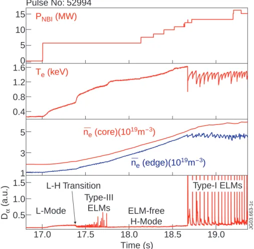
As can be seen on fig. 1.6, just after the L to H transition, one generally observes a series of bursts on the Dα signal1, whose frequency decreases in time. These bursts are associated to so-called “type III Edge Localized Modes (ELMs)”. If Pinj is large enough, type III ELMs are followed by a period of time where the Dα signal is quiet, which is called the “ELM-free H-mode”. A further increase in Pinj leads to large, quasi-periodic bursts on the Dα signal, which are the mark of “type I (or giant) ELMs”.

Good reviews on ELMs can be found in [10, 11, 12, 14, 20]. Here, we are particularly interested in type I ELMs. Indeed, the type I ELMy H-mode has been chosen as the

1_{The Dα} _{signal gives a measure of the emission of the α ray of deuterium which is associated to its}

recycling, i.e. its coming back into the plasma after having reached the PFCs. The Dαsignal is therefore a measure of the recycling, which is itself strongly correlated to the particle flux coming out from the plasma and reaching the PFCs.

(21)

Figure 1.5: Typical pressure profiles for the different operating modes in a tokamak.

baseline mode of operation for ITER, due mainly to its good confinement properties [35]. The main experimentally observed characteristics of type I ELMs are the following:

• They expulse a certain amount of particles and energy from the edge plasma (by

“edge” we mean here edge of the region inside the separatrix), resulting in a collapse of the profiles, as can be seen on fig. 1.7. Following this collapse, the profiles are re-built thanks to the energy and particle fluxes coming from the core as well as from local power sources and particles recycling and/or injection, until the next ELM happens.

• They are associated to magnetic fluctuations (observable with magnetic pick-up

coils located in the vacuum vessel [but away from the plasma]).

• Their typical duration is of the order of 200µs. • They are localized mainly on the LFS.

From the point of view of PFCs, ELMs in general and type I ELMs in particular are synonyms of large transient heat and particles loads. On fig. 1.8, the impact of type I ELMs on PFCs appears very clearly. As explained in section 1.6.1, these loads can cause damage to the PFCs and they are the reason for the need to avoid type I ELMs in ITER. Magnetohydrodynamics origin of the ELMs

On the theoretical viewpoint, type I ELMs have been found to be triggered by Mag-netoHydroDynamics (MHD) instabilities [15]. It is important to detail this somewhat,

(22)

1.5. THE H-MODE AND EDGE LOCALIZED MODES 21 0 10 5 1 3 5 15 0.5 0.4 0.8 1.2 1.6 1.0 1.5 17.0 17.5 18.0 18.5 19.0 Dα (a.u.) Time (s) JG03.663-1c Pulse No: 52994 P_NBI (MW) T_e (keV) L-Mode L-H Transition Type-III ELMs _ELM-free H-Mode ne (core)(1019m-3) n_e (edge)(1019m-3) Type-I ELMs

Figure 1.6: Overview on a JET discharge displaying the typical sequence of events during the gradual increase in the injected power. From [9].

Figure 1.7: Profiles of the electron density (left) and electron temperature (right) just before and just after a type I ELM.

(23)

Figure 1.8: Photographs of the vacuum vessel of the JET tokamak taken in visible light before (left) and during (right) an ELM. Visible light comes typically from the recycling deuterium (Dα ray) or from light impurities, so that the patterns observable on this figure are linked to

recycling and, indirectly, to the heat flux deposition (which is responsible for the release of light impurities from the plasma facing components). (courtesy Ph. Ghendrih)

(24)

1.5. THE H-MODE AND EDGE LOCALIZED MODES 23 because it will be useful in order to understand how ELMs control by Resonant Magnetic Perturbations (RMPs) works (or is thought to work, at least in certain cases - see section 2.2.2).

Let us first explain what MHD is. Generally speaking, there are several possible levels of description of a plasma. Due to the very low collisionality of tokamak plasmas, kinetic models, based on the Vlasov equation, are the most relevant ones. The gyrokinetic model, in which the dimensionality is reduced from six to five degrees of freedom by means of an averaging with respect to the gyromotion of the charged particles, is presently the subject of important efforts in the community. However, such models are hardly possible to tackle analytically, which is why numerical codes are being developed, but these codes also require large resources, due to the large number of degrees of freedom. A less refined but less demanding description of the plasma is obtained when taking the successive mo-ments of the Vlasov equation with respect to the particles velocity, which results in a fluid model. It is common, in particular in order to study the anomalous transport due to plasma turbulence, to use a description that considers the electrons and the ions as two separate fluids. But the model can be simplified further, so as to become a single-fluid model, called the MHD model. Even though the MHD model does not describe many important aspects of the plasma dynamics, it is still very utilized and is of great practical interest. In particular, this model is able to describe (at least partly) most of the main fast, large scale instabilities that are susceptible to occur in tokamaks and therefore limit the operational space in which to run them. Thus, the basic equilibrium of a tokamak plasma is in general calculated in the frame of MHD2_.

Ideal MHD [13] is the reduction of the MHD model where the plasma electrical re-sistivity is assumed to be null. In ideal MHD, the stability of the plasma can be studied through a so-called “energy principle” that we will briefly explain now. Linearizing the ideal MHD equations around an equilibrium state, all the perturbed quantities (magnetic field, current density, etc.) can be expressed as a function of the spatial displacement field of the plasma, ~ξ, with respect to its equilibrium position. It is thereby possible to define a potential energy δW that is a function of ~ξ only. The energy principle simply states that the plasma is stable if δW is positive for any possible ~ξ. The potential energy is calcu-lated in the form of an integral over the whole domain of the physical problem, which in general comprises a plasma region surrounded by a vacuum region, itself surrounded by a wall which is assumed to have an infinite electrical conductivity. The potential energy can be decomposed in the following way [13]:

δW = δWF + δWS+ δWV, (1.12) where δWF (resp. δWS, resp. δWV) denotes the contribution from the plasma (“F” stands for “fluid”) (resp. plasma-vacuum interface [“S” standing for “surface”], resp. vacuum). We will not give the expressions for δWS or δWV, the interesting elements for our purpose being contained in the expression of δWF:

2_{The Grad-Shafranov equation [2], which is the classical equation used in order to calculate the plasma}

(25)

δWF = 1 2 Z Z Z plasma dV£| ~Q⊥|2+ B2|~∇ · ~ξ⊥+ 2~ξ⊥· ~κ|2+ γp|~∇ · ~ξ|2 (1.13) − 2 ³ ~ξ⊥· ~∇p ´ ³ ~κ · ~ξ∗ ⊥ ´ − jkB−1 ³ ~ξ∗ ⊥× ~B ´ · ~Q⊥ ¤ .

In this expression, the integral is taken over the plasma volume, the indexes ⊥ and k designate the components perpendicular and parallel to the equilibrium magnetic field,

~

Q is the linear perturbation of the magnetic field ~B, ~κ is the curvature of the equilibrium

magnetic field (~κ ≡ (~b · ~∇)~b, with ~b ≡ ~B/B), γ (=5/3) is the ratio of specific heats of the

plasma, p is the plasma pressure, and ~j is the current density. Finally, stars designate complex conjugate quantities (all quantities are real a priori, but the expression pre-sented here is extended to cases where a Fourier transform is used). The energy principle provides an important insight on the physics at play in MHD instabilities in the sense that it allows one to identify clearly the sources of instability. Indeed, the first three terms under the integration symbol are positive definite, meaning that their contribution is always stabilizing, whereas the last two terms are susceptible to be negative, meaning that they can lead to an instability. Looking at the expression of those last two terms, the possible sources of instability turn out to be the pressure gradient3 _{and the parallel}

current density.

The evolution of research on linear ideal MHD related to type I ELMs is well described in [15]. The present model is the so-called “Peeling-Ballooning” (P-B) model, which deals with instabilities that are driven by both the parallel current density4 _(peeling

compo-nent) and the pressure gradient (ballooning compocompo-nent) in the pedestal. This model provides stability diagrams such as the one shown in fig. 1.9, where the stable and un-stable regions are shown in the (α, jped) space of parameters, α being the normalized pressure gradient in the pedestal and jped the parallel current density in the pedestal. Many experiments (see in particular [16]) have confirmed that type I ELMs are triggered when the plasma reaches the boundary between the stable and unstable zones in such diagrams.

1.6 ELMs control

1.6.1 The necessity of ELMs control for ITER

Estimation of the type I ELM size in ITER

As mentioned above, the type I ELMy H-mode is the reference scenario for ITER [35]. Studies have been done in the past years in order to estimate the ELMs size (from now

3_{Typically, the pressure gradient term is negative (destabilizing) on the LFS (where the pressure}

gradient and magnetic curvature point towards the same direction) and positive (stabilizing) on the HFS, explaining the tendency of some MHD instabilities to present a so-called “ballooning” aspect, i.e. to be localized on the LFS.

4_{It should be noticed that in the pedestal, the parallel current is essentially constituted by bootstrap}

(26)

1.6. ELMS CONTROL 25

Figure 1.9: Example of the MHD P-B stability as a function of the normalized radial pres-sure gradient in the pedestal (α) and the current density in the pedestal normalized to its experimental value for a JET H-mode discharge. Each square marks an equilibrium for which the stability was evaluated. The small black squares indicate instability of n = ∞ (n being the toroidal mode number of the mode - and n = ∞ thus corresponding to modes infinitely localized perpendicularly to the equilibrium magnetic field) ballooning modes while the large coloured squares indicate instabilities with a finite n, the colour depending on the value of n. From [15].

(27)

on, “ELMs” will always mean “type I ELMs”, unless precised), i.e. the amount of energy expelled from the confined region during an ELM, ∆WELM, in ITER [17]. The estimation is based on an experimental approach. Data was collected from the largest tokamaks in the world in order to determine the physical parameters that have an influence on the ELM size. A clear scaling of the ELM size normalized to Wped, the amount of energy “stored in the pedestal”5_{, with the plasma pedestal electron collisionality ν}∗

e (defined as ν∗

e ≡ πRqλe,e95, where λe,e is the electron-electron collision mean free path [2] calculated

with the values of the pedestal parameters) was found and is illustrated on fig. 1.10. As one can see on this figure, the ELM size increases as collisionality decreases. At the ITER value for ν∗

e, which is about 0.1, the normalized ELM size is of about 15%, which corresponds to ∆WELM ' 17MJ (since Wped' 110MJ in ITER).

Maximum tolerable type I ELM size in ITER

In parallel, work was done in order to estimate the consequences of the ELMs on the ITER PFCs, depending on their size [18, 19]. The conclusion from Federici et al. [18] was that the maximal tolerable size for the ELMs6 _{was of about 3 or 4MJ. This was}

al-ready far below the expected 17MJ, but recent work [19] reduces even more the tolerable ELM size, now considered to be below 2MJ.

The conclusion is that type I ELMs are unacceptable in ITER, which is in obvious con-tradiction with the fact to take the type I ELMy H-mode as the reference scenario.

1.6.2 Possible solutions to the problem of ELMs

Benefic effects of type I ELMs

Before describing the different possible solutions that have been imagined in order to solve the problem of ELMs in ITER, it is important to mention that, although ELMs are nefast to PFCs, they have certain benefic effects. In particular, by transiently ex-pelling large amounts of particles from the confined plasma, they maintain a certain level of density and impurity transport at the edge. Without ELMs, it would be difficult to prevent the density from rising too much7 _{and the impurities (and also fusion “ashes”,}

i.e. α particles) to accumulate in the core plasma8_{. Furthermore, the type I ELMy}

H-mode, in spite of the ELMs, presents good confinement properties and a good level

5_{defined as Wped} _≡ 3

2ne,ped(Te,ped + Ti,ped)Vplasma, where ne,ped (resp. Te,ped, resp. Ti,ped) is the

plasma density (resp. electron temperature, resp. ion temperature) at the top of the pedestal and

Vplasma is the volume of the confined plasma

6_{By “tolerable size” we mean the size allowing the divertor to survive for about 3000 discharges}

(∼ 106_{type I ELMs) at full injected power. This duration corresponds to the ITER divertor replacement}

schedule.

7_{A too high density is a well known cause of disruption, i.e. abrupt, undesired, termination of the}

discharge.

8_{Impurities are species others than the species “normally” present in the plasma (i.e. deuterium,}

tritium and α particles), for instance carbon, nickel or oxygen. In general, they come from the PFCs, and are nefast to the plasma because they disperse a large amount of power by radiation (especially the heavy impurities), thereby cooling down the plasma (and in some cases leading to a radiative collapse of the plasma), and also they dilute the “fuel”, i.e. the deuterium and tritium mixture, reducing the fusion power. The same problems exist with α particles.

(28)

1.6. ELMS CONTROL 27

Figure 1.10: Typical amount of energy expelled during a type I ELM nomalized to the pedestal energy, as a function of the pedestal electron collisionality, for different large tokamaks. The domains of collisionality explored during the DIII-D ELMs control experiments (see chapter 2) are shown in purple. From [29].

of fusion power, which is the reason why it was chosen as the reference scenario for ITER. Looking for a way to avoid the ELMs, one should thus make sure that a sufficient level of particle transport will still exist and that the plasma performances will not be degraded.

Passive or active ELMs control methods

Now, there are two possible approaches to try and avoid the ELMs. The first one, which we could call “passive control approach”, consists in looking for another regime in which to run ITER that would offer similar performances to the type I ELMy H-mode but would not damage the PFCs so drastically. The second one, the “active control approach”, consists in keeping the type I ELMy H-mode as the ITER baseline scenario, but controlling the ELMs (i.e. either reducing their size or totally suppressing them) by dedicated means. Several variations of these two concepts have been investigated and are reviewed in [14, 20, 35]. Different high confinement scenarios without type I ELMs have been found in present machines. However, the extrapolation of these regimes to ITER is questionable since the operational windows are usually very narrow and do not match ITER relevant parameters. Active ELMs control methods are thus likely to be required in ITER. The two main candidates are ELMs triggering by pellet injection [21] and ELMs mitigation by Resonant Magnetic Perturbations (RMPs), the central subject of the present manuscript. It has been decided to implement both systems in ITER.

(29)

1.7 ELMs control by Resonant Magnetic

Perturba-tions

We now focus on the central subject of this work: ELMs control by RMPs. In this section, we explain the “historical” genesis of the concept.

1.7.1 Degrading the ETB to suppress ELMs

The underlying idea is that, according to the ideal MHD theory of ELMs9 _{presented in}

section 1.5.2, ELMs occur because the Edge Transport Barrier (ETB) of the H-mode is “too efficient”, i.e. the pressure gradient, and hence bootstrap current density, can reach too large values. If, by some process, transport in the ETB could be enhanced enough that the plasma would remain in the stable region with respect to P-B instabilities (however without loosing all the benefit of the ETB if possible!), ELMs could be avoided10_.

1.7.2 Confinement degradation by radial RMPs

One possible way to enhance the radial transport in a tokamak is to produce magnetic perturbations that possess a radial component. That way, the very efficient parallel transport contributes to the radial transport. It is known in particular that radial RMPs (“resonant” means constant along field lines on a given flux surface, called “resonant surface”), can “tear” the nested flux surfaces, creating so-called “magnetic islands” [2], a schematic example of which can be seen on fig. 1.11. When a magnetic island is present inside the plasma, the radial transport is short-circuited, across the island width, by the strong parallel transport. Thus, in terms of transport, the annulus of plasma located in the region of the island is effectively “lost”, because it offers almost no resistance to radial transport. That is why, usually, one tries to avoid large magnetic islands inside the plasma. However, for our purposes, magnetic islands could be beneficial.

1.7.3 Ergodic divertors

Islands overlapping and ergodic magnetic field

It can happen that several islands chains exist in the plasma, centered on distinct resonant surfaces. This is the case in fig. 1.12, which presents three Poincar´e plots done for RMPs containing only (m = 2, n = 1) and (m = 3, n = 2) components, m (resp. n) being the poloidal (resp. toroidal) mode number, which create islands chains on the q = 2 and

q = 3/2 surfaces. The three Poincar´e plots correspond to three amplitudes of the RMPs,

more precisely there is an increase of the RMPs by a factor 2 between the top and the middle plots as well as between the middle and the bottom plots. It can be seen that for small enough RMPs, the islands are well separated, but that increasing the RMPs, the islands grow until they “overlap”. Then, magnetic field lines start to behave in a chaotic

9_{which was, as mentioned above, validated by many experiments}

10_{An important remark here is that several of the high confinement scenarios alternative to the type}

(30)

1.7. ELMS CONTROL BY RMPS 29

Figure 1.11: Schematic poloidal cut of a circular plasma showing several flux surfaces. An islands chain appears with its separatrix in red, while the position of the previous resonant surface (before the islands chain existed) is shown by a dash-dotted black line.

manner, all closed flux surfaces between the two resonant surfaces being destroyed11_{. One}

will also often find the words “stochastic” and (for instance in the rest of this manuscript) “ergodic”, which are used with almost no distinction in the fusion community, although they have a different mathematical meaning [43]. The degree of islands overlapping is quantified by the so-called “Chirikov parameter”, σChir, which, in-between two islands chains of radial half-widths δ1 and δ2 separated by a radial distance ∆12, is defined as:

σChir ≡

δ1+ δ2

∆12

. (1.14)

The criterion for ergodicity to occur is therefore σChir ≥ 1, roughly.

In the past, several machines have tested the concept of “ergodic limiter” (see the review paper [33]). This is still the case today in the TEXTOR tokamak. The idea is to use a specific set of coils to produce radial RMPs at the edge of the plasma, so as to create an ergodic region, for the purpose of improving the plasma-wall interaction with respect to a standard limiter case.

11_{This description is somewhat simplified. In fact, before the islands overlap, there are higher order}

islands chains (i.e. islands chains that appear at flux surfaces that are not resonant with the imposed RMPs) growing in-between them, as can be seen in fig. 1.12 (in particular on the middle plot). This process is described in [43]. The image of two “primary” islands chains (such as the (m = 2, n = 1) and (m = 3, n = 2) one on fig. 1.12) growing in the middle of nested flux surfaces until they overlap is thus incorrect, although it is intuitively helpful.

(31)

0 1 2 3 4 5 6 0.7 0.75 0.8 0.85 0.9 0.95 theta* s 0 1 2 3 4 5 6 0.7 0.75 0.8 0.85 0.9 0.95 theta* s 0 1 2 3 4 5 6 0.7 0.75 0.8 0.85 0.9 0.95 theta* s

Figure 1.12: Poincar´e plots obtained by field line integration. θ∗is a poloidal coordinate and s a radial coordinate. The RMPs only have an (m = 2, n = 1) and an (m = 3, n = 2) components, which create two islands chains on the q = 2 and the q = 3/2 surfaces. Between the top and middle plots, as well as between the middle and bottom plots, the amplitude of the RMPs is doubled.

(32)

1.8. CONSTRUCTION OF THE PRESENT MANUSCRIPT 31

1.7.4 Synergy between the axisymmetric poloidal divertor and

the ergodic divertor

As is well known (see for instance [2] or appendix A), for a given RMPs amplitude, the islands widths scale as (q0₎−1/2_{, q}0 _{being the magnetic shear, i.e. the radial derivative} of the safety factor q, while the distance between islands chains scales as (q0₎−1_{. The} Chirikov parameter therefore scales as (q0₎1/2_{, meaning that a high magnetic shear is}

favorable for ergodization. As mentioned above, for poloidally diverted plasmas q tends to infinity when approaching the separatrix, and so does q0_{. The magnetic field at the} edge is likely to be ergodized easily. Reference [24] provides a good illustration that a poloidally diverted plasma is more easily subject to edge ergodization than a plasma in limiter configuration.

1.7.5 Transport in an ergodic magnetic field

The main theoretically expected effect of the magnetic field ergodization on radial trans-port is an enhancement of the heat transtrans-port through the electrons [23], which travel along field lines much faster than the ions (at equal temperatures, their thermal velocity is larger than that of the ions by a factor (mi/me)1/2) and hence have larger parallel trans-port coefficients. This effect was verified experimentally in several devices, as reviewed in [33]. An increase in the density transport is also expected and was clearly observed experi-mentally [33], sometimes resulting in a “pump-out”, i.e. a drop in the plasma density [34]. The conclusion of the above considerations is that it seems a priori worthwile trying to ergodize the magnetic field at the edge of an H-mode tokamak plasma in order to increase the pedestal transport and, hopefully, suppress type I ELMs. This was the statement of Grosman et al. in 2003 [62], who proposed to test the concept at DIII-D. In next chapter, we will see that this concept was indeed tested (and is still under inves-tigation) at DIII-D and led to ELMs suppression, although not exactly in the way that was imagined by Grosman et al..

1.8 Construction of the present manuscript

The manuscript is constructed as follows. In chapter 2, we review the experimental and modelling findings from the DIII-D experiments using the so-called “I-coils” in order to mitigate the ELMs. These experiments are the departure point of the present work. In chapter 3, we describe the numerical tools that we developed in order to calculate and analyze the magnetic perturbations created by a given set of coils in a tokamak plasma and describe our results for the DIII-D I-coils. In chapter 4, we present recent experiments on ELMs mitigation by RMPs done at JET and MAST with the error field correction coils in which we participated and provided modelling support using the tools presented in chapter 3. In chapter 5, we report on our design study for ELMs control coils for ITER, the central piece of the present manuscript from a practical point of view. This design study was indeed used in the ITER design review process, which led to the decision to implement ELMs control coils in ITER (although it is not yet decided which design

(33)

will be chosen). Finally, in chapter 6, we present our modelling work for ELMs control experiments, using non-linear MHD numerical simulations, a necessary tool in order to understand the plasma response on the external RMPs and progress in the understanding of the physical mechanisms at play in ELMs control by RMPs.

(34)

Chapter 2 ELMs control with the I-coils at

DIII-D

In 2003, DIII-D was the first tokamak to demonstrate the possibility to control the ELMs by imposing RMPs to the plasma, using a set of coils called the “I-coils”. After having briefly described these coils, we will present the experimental phenomenology and describe the present status of modelling and interpretation of the experiments.

2.1 The DIII-D I-coils

The I-coils [41] are a set of 12 coils located inside the vacuum vessel (“I” standing for “internal”) of DIII-D that were originally installed in order to stabilize the so-called “re-sistive wall modes” (see section 5.2 for a brief definition of these modes). A schematic view of the DIII-D I-coils appears on fig. 2.1. On this figure, one can see that there are two rows of six coils equally spaced toroidally, the two rows being symmetric with respect to the midplane (the horizontal plane containing the magnetic axis). The current direc-tion alternates between one coil and the toroidally adjacent one. The coils thus produce mainly n = 3 magnetic perturbations. The coils are single turn loops which can carry up to 7kA (but in most of the past experiments, the current was limited to ∼ 4kA). There are two possible configurations: in the so-called “even parity” configuration, the upper and lower coils are in phase (i.e. the current flows in the same direction in upper and lower coils that are at the same toroidal location, those coils hence producing a radial magnetic perturbation pointing in the same direction), and in the “odd parity” configuration they are out of phase (or shifted by 60◦ _{toroidally, which is equivalent). Both these} configura-tions have been used in the experiments, with different effects on the plasma, as will be detailed below. Calculations of the (vacuum-like, i.e. neglecting any plasma response) magnetic perturbations produced by both configurations are presented in chapter 3 and show that the even parity configuration produces stronger RMPs than the odd parity one.

2.2 The experiments

It is usual to distinguish the DIII-D ELMs control experiments with the I-coils according to the value of the electron pedestal collisionality ν∗

e (see section 1.6.1 for a definition

(35)

Figure 2.1: Left: 3D schematic view of the DIII-D I-coils together with the shape of a typical DIII-D plasma. Right: photograph taken inside the DIII-D vacuum vessel with one of the I-coils highlighted in red. From [36].

of ν∗

e). Indeed, as can be seen on fig. 1.10, two distinct domains of collisionality were explored: one “high collisionality” domain (ν∗

e ∼ 1) [25, 26, 27, 28] and one “low col-lisionality” domain (ν∗

e ∼ 0.1, close to the ITER forecasted value) [28, 27, 30, 31, 32]. These two domains were explored successively in time: the high ν∗

e one in 2004 mainly, and the low ν∗

e one since 2005. While the high νe∗ experiments used the odd parity I-coils configuration, the low ν∗

e ones were mainly done with the even parity configuration1. In both domains, the I-coils were shown to have a very clear effect on the ELMs but the phenomenology was somewhat different. In the following sections, we describe the high and low ν∗

e experiments successively. Each time, we present the phenomenology in a first subsection and we summarize modelling results and elements of interpretation in a second subsection.

2.2.1 High collisionality experiments

As stated above, the high ν∗

e (∼ 1) domain was explored first [25, 26, 27, 28], using the odd parity configuration of the I-coils, which produces much smaller RMPs than the even parity one (see section 3.2).

Phenomenology

On fig. 2.2 (second box from the top), it can be seen that ELMs suppression occurs immediately after the beginning of the I-coils pulse (or more precisely within 15ms, i.e. less than one typical ELM cycle), but that ELMs are not completely suppressed: some large Dα spikes remain. No difference was found between the remaining ELMs during the I-coils pulse and the ELMs before the I-coils pulse.

1_{It should be noticed that changing the I-coils configuration from odd to even (or vice versa) requires}

hardware modifications, so that the configuration cannot be changed between, for instance, two shots on the same experimental day. The fact that the high ν∗

e experiments were done in the less resonant odd parity configuration is only due to the fact that this was the configuration in which the I-coils were used at the time for other purposes. When ELMs control by RMPs became a high priority subject on DIII-D, the I-coils were switched to the even parity configuration and stayed that way until now.

(36)

2.2. THE EXPERIMENTS 35

Figure 2.2: Experimental times traces for two shots: one at high ν∗

e (115467, black traces), the

other at low ν∗

(37)

In-between the remaining ELMs, one can see that the Dα signal is not completely quiet. A detailed study reveals that the Dαsignal in fact presents a bursty behaviour modulated with a coherent 130Hz envelope. This is associated with magnetic fluctuations (measured by magnetic probes) that also present a bursty behaviour with a coherent 130Hz envelope. The H98(y,2) confinement factor2 (bottom box on fig. 2.2) remains constant during the

I-coils pulse, meaning that the I-coils do not degrade the energy confinement. This is a strong point in favor of an application to ITER.

Consistently, the ETB does not seem to be affected by the I-coils and the temperature and density profiles exhibit only small changes between before and during the I-coils pulse, as can be seen on fig. 2.3.

On the other hand, the toroidal rotation profile shows a clear braking of the plasma due to the I-coils -see fig. 2.5- and in particular the toroidal rotation at the foot of the pedestal is reduced to zero.

Plasma current ramp experiments were done in order to investigate the dependence of the results on q95[28]. It was found that ELMs suppression is only obtained for 3.5 ≤ q95 ≤ 3.9

(with an optimal suppression at q95' 3.7)3.

The magnetic footprints (i.e. regions of high heat and particle fluxes on the divertor plates, see section 4.2.2) exhibit a clear change between before and during the I-coils pulse, with a so-called “triple splitting” of the strike points [59].

Finally, it should be noticed that the plasma behaviour is sensitive to the toroidal phase of the magnetic perturbations from the I-coils (which can be changed by 60◦ _{by reversing} the direction of current in all the coils).

Modelling and interpretation

The fact that the remaining ELMs during the I-coils pulse present no obvious difference with the “natural” ELMs suggests that the I-coils do not directly affect the ELMs, but only the transport in-between ELMs. Accordingly, a transport analysis [26] indicates that, in-between the remaining ELMs, an extra-transport mechanism (possibly related to the bursty Dα and magnetic fluctuations observed) is at play that slows down the recovery time of the profiles between ELMs and thus reduces the ELMs frequency. Somewhat paradoxically, calculations of the vacuum-like magnetic perturbations pro-duced by the I-coils in odd parity configuration, which are presented in chapter 3, show that the experimental q95 window for ELMs suppression corresponds to a “valley” in

the odd parity I-coils magnetic perturbations spectrum, with edge ergodization occurring only on the ∼ 2% most external flux surfaces4_{. This could mean that edge ergodization}

is not the reason of ELMs suppression. On the other hand, the observed drop in the toroidal rotation is consistent with a penetration of the RMPs, according to the classical theory of RMPs penetration into a rotating plasma (see chapter 6), and a modelling of the magnetic footprints [59] reveals that the observed splitting of the strike points is larger than the one calculated in the vacuum field hypothesis, meaning that there could

2_{which is defined as the ratio of the discharge thermal energy confinement time τth} _{to a reference}

energy confinement time τth,98y2given by a scaling law that is derived from many experiments in present machines and used for ITER predictions, see [35]

3_{The resonant window was however observed to change with the shape and pedestal parameters of}

the discharge.

(38)

Figure 2.3: (a) Electron density (ne) and (b) temperature (Te) profiles averaged over 100ms

before (at t = 2900ms) and during (at t = 3300ms) the I-coil pulse for shot 115467 and at

t = 3300ms for shot 115468, where there was no I-coils pulse. (c) Ion temperature (Ti) profile

(39)

be a plasma response amplifying the external RMPs.

To finish, the sensitivity of the experimental results to the phase of the magnetic per-turbations suggests that there exist intrinsic “error fields” (coming for instance from misalignments of the toroidal or poloidal field coils or currents flowing in the coils ali-mentation systems), which play a non negligible role.

2.2.2 Low collisionality experiments

Since 2005, DIII-D ELMs control experiments are devoted to the low ν∗

e domain [28, 27, 30, 31, 32], which is more relevant for ITER. In order to reach this domain, an active pumping by a cryopump is used so as to decrease the plasma density5_{. For the pumping}

to be efficient, the plasma shape is chosen such that the outer strike point is located near the entrance of the cryopump.

Phenomenology The very first low ν∗

e experiments were done with the I-coils in odd parity configuration [28, 27]. An effect on the ELMs was observed, typically an increase in their frequency by a factor of about 2 and decrease in their amplitude by an order of magnitude. However, this configuration was not studied much.

Indeed, the I-coils configuration was soon switched to the even parity one, which is by far more resonant (see section 3.3.2). This configuration is being studied in detail since 2005 and we participated on-site to some of the experiments.

As can be seen on fig. 2.2 (top box), a complete suppression of the ELMs (no remaining spike on the Dα signal) occurs during the I-coils pulse but there is some delay with re-spect to the beginning of the I-coils pulse before the ELMs completely disappear. This is clearly different from the high ν∗

e experiments, were the suppression was incomplete but immediate6_.

One common point, however, between low and high ν∗

e, is that the H98(y,2) confinement

factor (bottom box on fig. 2.2) is not affected by the I-coils.

Looking at the plasma profiles (fig. 2.4), a clear “pump-out” (decrease in ne) due to the I-coils can be observed. The electron temperature (Te) profile is flattened for a normalized poloidal flux ψN (used here as a radial coordinate) below ∼ 0.97 and the Te pedestal is conserved, with even a slight increase with the I-coils current II−coils in the value of Teat the top of the pedestal. Furthermore, the width of the pedestal decreases with increasing

II−coils. There is thus a dramatic increase in |∂rTe| at the edge with II−coils. The ion temperature Ti is seen to increase with II−coils across the entire plasma edge and |∂rTi| increases strongly for ψN > 0.97.

The toroidal velocity is also typically observed to increase at the edge in presence of the RMPs (fig. 2.5), oppositely to the high ν∗

e results. In the core, however, a drop in the rotation is still observed [36].

5_{Without pumping, all of the particles escaping the plasma tend to recycle, i.e. come back to the}

plasma, after reaching the plasma facing components, and density can thus not be decreased significantly.

6_{This could be due to the fact that the time of penetration of the RMPs into the plasma is longer}

in that case due to the smaller plasma resistivity, an effect which will be seen in the non-linear MHD simulations presented in chapter 6.

(40)

Figure 2.4: Plasma profiles from three low ν∗

e shots with three different values of II−coils:

0kAt (reference case, black traces), 2kAt (red traces) and 3kAt (green traces). The normalized poloidal flux is used as a radial coordinate. From [29].

Figure 2.5: Toroidal rotation frequencies (in kilo-turns per second) for two shots: one at high

ν∗

Modélisation non-linéaire du transport en présence d'instabilité MHD du plasma périphérique de tokamak.

HAL Id: pastel-00003137

https://pastel.archives-ouvertes.fr/pastel-00003137

d’instabilité MHD du plasma périphérique de tokamak.

Eric Nardon

To cite this version:

Th`

ese de doctorat de l’´

Ecole Polytechnique

Physique

´

Eric NARDON

EDGE LOCALIZED MODES CONTROL

BY RESONANT MAGNETIC PERTURBATIONS

CONTR ˆ

OLE DES INSTABILIT´

ES DE BORD

PAR PERTURBATIONS MAGN´

ETIQUES R´

ESONANTES

Remerciements

Summary

R´

esum´

e

Contents

Chapter 1

Introduction

1.1

General introduction to fusion

1.2

The tokamak configuration

1.3

ITER

1.4

Transport in tokamaks

1.4.1

Parallel versus perpendicular transport

1.4.2

Drifts

1.4.3

Turbulence

1.5

The H-mode and Edge Localized Modes

1.5.1

The H-mode

1.5.2

Edge Localized Modes

1.6

ELMs control

1.6.1

The necessity of ELMs control for ITER

1.6.2

Possible solutions to the problem of ELMs

1.7

ELMs control by Resonant Magnetic

Perturba-tions

1.7.1

Degrading the ETB to suppress ELMs

1.7.2

Confinement degradation by radial RMPs

1.7.3

Ergodic divertors

1.7.4

Synergy between the axisymmetric poloidal divertor and

the ergodic divertor

1.7.5

Transport in an ergodic magnetic field

1.8

Construction of the present manuscript

Chapter 2

ELMs control with the I-coils at

DIII-D

2.1

The DIII-D I-coils

2.2

The experiments

2.2.1

High collisionality experiments

2.2.2