HAL Id: hal-01825267
https://hal.univ-lorraine.fr/hal-01825267
Submitted on 28 Jun 2018HAL is a multi-disciplinary open access
archive for the deposit and dissemination of sci-entific research documents, whether they are pub-lished or not. The documents may come from teaching and research institutions in France or abroad, or from public or private research centers.
L’archive ouverte pluridisciplinaire HAL, est destinée au dépôt et à la diffusion de documents scientifiques de niveau recherche, publiés ou non, émanant des établissements d’enseignement et de recherche français ou étrangers, des laboratoires publics ou privés.
A workflow for 3D stochastic modeling of salt from
seismic images
Nicolas Clausolles, Pauline Collon, Guillaume Caumon
To cite this version:
Nicolas Clausolles, Pauline Collon, Guillaume Caumon. A workflow for 3D stochastic modeling of salt from seismic images. 80th EAGE Conference and Exhibition 2018, Jun 2018, Copenhagen, Denmark. 2018. �hal-01825267�
Nicolas Clausolles1, Pauline Collon1, and Guillaume Caumon1
1Universit´e de Lorraine, CNRS, GeoRessources, F-54000 Nancy, France
June 2018
Abstract
Interpreting salt is a complex and time consuming task in seismic interpretation. Considerable progresses have been made recently by automatic methods which detect deterministic salt tops from the seismic image. However, uncertainties about salt exist, owing to intrinsic physical limitations of seismic imaging. Therefore, we propose a new workflow to generate several possible models of salt top surfaces with varying geometries and topologies. The method we propose is divided into three steps. We first segment the seismic volume into three regions: salt, sediments and uncertain, depending on the reliability of the automatic interpretation. We then compute a monotonic scalar field in the uncertain region, ranging from zero at the contact with salt to one at the contact with sediments. We finally generate a random field bounded between zero and one. The salt boundary is implicitly defined by the zero isovalue of the scalar field defined as the difference between the distance and the random fields. Applications of this workflow on a 2D seismic image and a 3D synthetic data set illustrate the potential of the method to efficiently address salt interpretation uncertainties.
80th EAGE Conference and Exhibition 2018
1
Introduction
Salt has always been challenging in seismic imaging due to both its physical properties and the complex geometries and topologies it forms. Its interpretation is a long and iterative process, mostly manually done. Over the last decades, seismic acquisition and processing methods have considerably improved, leading to denser and better resolved seismic amplitude volumes. These progresses motivated a lot of works on the automation of salt interpretation (e.g., Aqrawi et al., 2011; Berthelot et al., 2013; Wu, 2016; Di & AlRegib, 2017; Waldeland & Solberg, 2017; Hauk˚as et al., 2017, among the most recent). This automation has certain advantages, such as a significant reduction of the time spent on the interpretation and of the possible human conceptual biases. The methods proposed in the literature often provide, however, a single interpretation - the ”best” one - of salt boundaries according to the available data. Such deterministic approaches prevent from exploring the different structural scenarios that could be admissible given the imaging uncertainties (e.g., interpreting a thin diapir stock or a weld). Furthermore, as compared to manual interpretation, automatic interpretation is a purely computational process that does not explicitly introduce any geological knowledge.
Different alternatives have been proposed to overcome these limitations. Wu (2016) proposes to take into account manually picked samples to guide the interpretation in complicated zones. Hauk˚as et al. (2017) extract surface patches in the well-defined boundary zones and then connect the different patches by classifying the seismic data into ”salt”, ”sediments”, and ”uncertain” and extrapolating the surface patches in the ”uncertain” region.
In this paper, we propose a first general workflow that aims at generating different possible models of salt top surfaces from seismic images. As Hauk˚as et al. (2017), we partition the seismic volume into ”salt”, ”sediments” and ”uncertain” to determine the zone that contains the salt boundary. We then use a perturbed distance-based method to generate different top salt surfaces. We illustrate the workflow on a 2D seismic image and present a simple example on a 3D synthetic salt diapir. We finally discuss some technical points about the method, such as data conditioning and the choice of simulation parameters.
2
Method
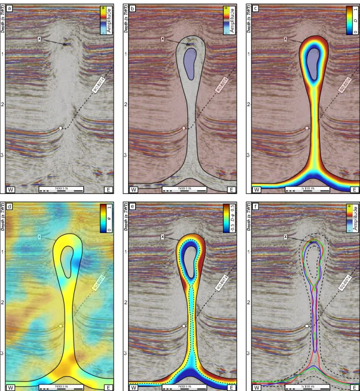
The first step of our method is to define the regions of the seismic cube for which we consider the interpretation as sure (Fig. 1.a and 1.b). Two regions are defined: the ”salt” region, and the ”sedi-ments” region. The remaining samples, that are expected to lie in between those two regions, define a third ”uncertain” region that encompasses the salt boundary. We do not develop in this paper how to generate these three regions. Different automatic methods are already proposed in the literature to extract salt geobodies from seismic images. These methods are often based on either attribute extrema extraction (Wu, 2016) or attribute classification (Berthelot et al., 2013; Di & AlRegib, 2017; Waldeland & Solberg, 2017) and can be adapted to ignore the uncertain samples around the boundary. The most straightforward method may be to compute an attribute representing the probability of having salt (e.g., Wu, 2016), and to define the three regions by thresholding this at-tribute. From this step, our calculations will only focus on the ”uncertain” region, which we consider to contain the salt boundary.
To generate different salt boundary realizations, we use a variant of the Object-Distance Simulation method (Henrion et al., 2010; Rongier et al., 2014). Each realization is characterized by two scalar fields: a ”distance” field D (Fig. 1.c) that is common to all the realizations, and a random field ϕ (Fig. 1.d) that varies from one realization to an other. In our case, the ”distance” field D does not represent a true distance. It is a monotonically varying field ranging from zero at the contact with the ”salt” region and the base to one at the contact with the external ”sediments” region. It can be seen as a relative normalized distance of each sample to salt or, in other words, as the probability for each sample to be outside the salt boundary (i.e., to be sediments). This scalar field is obtained by: (1) setting to 0 the value of the samples in contact with the ”salt” region and the base, (2) setting to 1 the value of the samples in contact with the ”sediments” region, and (3) interpolating the intermediate values in the remainder of the region. In this paper, we use the Discrete Smooth Interpolation method (Mallet, 2002) for this interpolation.
The second scalar field, denoted ϕ, represents a spatially correlated perturbation that will be applied to the field D. The values of ϕ must satisfy the same range as the values of D, that is to say
a W E b W E f W E 0 D 1 c W E 0 φ 1 d W E -0.5 D-φ 0.5 e W E
Figure 1: Illustration of the method. The input seismic data (a, image from Jackson & Lewis, 2012) are segmented into three categories (b): sediments (red), salt (blue) and un-certain (uncolored). A normalized ”distance” field D (c) and a normalized perturbation field ϕ (d) are then generated in the uncertain region. The salt boundary (e, dashed curve) is obtained by extracting the zero isovalue of the difference between D and ϕ (e). Different salt boundaries (f) can be obtained by generating different random fields (the three realizations
share the same SGS parameters).
zero to one. In this paper, we use sequential Gaussian simulations (SGS) to generate the perturbation fields. The distribution model used for the SGS is a centered triangular distribution and the variogram model is assumed isotropic.
80th EAGE Conference and Exhibition 2018
difference of D and ϕ (Fig. 1.e):
SB : {x | D(x) − ϕ(x) = 0}. (1)
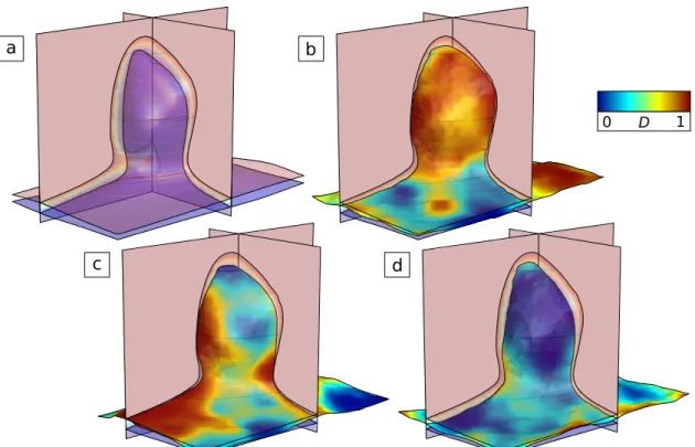
It can be further extracted using marching cubes to obtain an explicit representation of the boundary. Fig. 2 illustrates the application of the method on a 3D synthetic data set.
a b
c d
1 0 D
Figure 2: Synthetic example of a 3D salt diapir. The distance field D is computed from the boundaries of the uncertain envelope (a: red and blue surfaces). Running several simulations generates different top salt surfaces (b, c and d). The colormap corresponds to the distance
field D.
3
Discussion
The method proposed in this paper has the advantage of resting on a simple principle. This makes it easy to adjust to more specific purposes. First, it can be constrained to well data and seismic manual interpretation. In the example we present, we use unconditional SGS as we do not have any punctual salt top data to honor. However, well markers and deterministic seismic picks can easily be treated as conditioning data for the SGS (by setting at data location the value of the random field ϕ to the value of the normalized distance field D).
Secondly, the choice of the parameters used for the SGS will affect the geometry of the simulated boundary. As an example, the choice of the distribution model will determine the position of the boundary and thus the simulated volumes. In the example presented in Fig. 1, we used a centered triangular distribution. If we change it to a uniform or truncated Gaussian distribution model, it would affect the variance of the simulated volumes. Moreover, such distributions ensure that the simulated boundaries are statistically centered in the envelope. To generate models that are statistically closer to salt or sediments, we would need to use non-centered distribution models.
The choice of the variogram model affects the smoothness of the simulated boundaries: the larger the range is, the smoother the boundary is. Using a small variogram range may also trigger the apparition of blobs (green realization on Fig. 1.f). These blobs can be either preserved (e.g., to represent salt lenses remaining in a weld), or suppressed in a post-processing phase. In Fig. 1, we constrained the distance field D by a line set to 0.5 to allow for a continuous salt body. This could also
be obtained by using a locally variable anisotropy model for the random field (with a large variogram range orthogonally to the distance field gradient and a smaller range along the gradient). It would also prevent the random field ϕ of having sharp contacts with the uncertain envelope boundaries, which would produce unrealistic geometries. The choice of the SGS parameters can be partly calibrated from analogs (Henrion et al., 2010; Rongier et al., 2014).
4
Conclusions
The method we propose in this paper generates stochastic interpretations of salt geobody boundaries reflecting seismic imaging uncertainties. It can simulate both connected and unconnected salt bodies, although further work is needed to consider singularities such as salt welds during the simulation. The method can easily be conditioned to preexisting observations, such as seismic picks and well markers. A proof of concept has been presented on a basic synthetic 3D salt diapir. Further works will focus in the short term on providing a 3D workflow that fully automates the method, from the seismic volume segmentation to the extraction of the boundaries. This will make it possible to address the impact of geometrical and topological salt interpretation uncertainties in geophysical imaging and basin modeling.
5
Acknowledgements
This work was performed in the frame of the RING project at Universit´e de Lorraine. We would like to thank for their support the industrial and academic sponsors of the RING-GOCAD Consortium managed by ASGA. The software corresponding to this paper is available in the Goscope plugin of SKUA-Gocad. We also acknowledge Paradigm for the SKUA-Gocad Software and API.
References
A. A. Aqrawi, T. H. Boe & S. Barros [2011]. Detecting salt domes using a dip guided 3D Sobel seismic attribute. In: SEG Technical Program Expanded Abstracts 2011, pp. 1014–1018. Society of Exploration Geophysicists.
A. Berthelot, A. H. S. Solberg & L.-J. Gelius [2013]. Texture attributes for detection of salt. Journal of Applied Geophysics, 88:52–69. doi:10.1016/j.jappgeo.2012.09.006.
H. Di & G. AlRegib [2017]. Seismic Multi-attribute Classification for Salt Boundary Detection - A Comparison. In: 79th EAGE Conference and Exhibition 2017, June 2017. European Association of Geoscientists and Engineers. doi:10.3997/2214-4609.201700919.
J. Hauk˚as, A. Bounaim & O. Gramstad [2017]. Automated salt interpretation, Part II : Smooth surface wrapping of volume attribute. In: SEG Technical Program Expanded Abstracts 2017, pp. 2076–2080.
V. Henrion, G. Caumon & N. Cherpeau [2010]. ODSIM: An Object-Distance Simulation Method for Conditioning Complex Natural Structures. Mathematical Geosciences, 42(8):911–924. doi:10. 1007/s11004-010-9299-0.
C. A.-L. Jackson & M. M. Lewis [2012]. Origin of an anhydrite sheath encircling a salt diapir and implications for the seismic imaging of steep-sided salt structures, Egersund Basin, Northern North Sea. Journal of the Geological Society, 169(5):593–599. doi:10.1144/0016-76492011-126.
J.-L. Mallet [2002]. Geomodeling. Oxford University Press.
G. Rongier, P. Collon-Drouaillet & M. Filipponi [2014]. Simulation of 3D karst conduits with an object-distance based method integrating geological knowledge. Geomorphology, 217:152–164. doi:10.1016/j.geomorph.2014.04.024.
A. U. Waldeland & A. H. S. Solberg [2017]. Salt classification using deep learning. In: 79th EAGE Conference and Exhibition 2017, June 2017. European Association of Geoscientists and Engineers. X. Wu [2016]. Methods to compute salt likelihoods and extract salt boundaries from 3D seismic